Influence of Wake Model Superposition and Secondary Steering on Model-Based Wake Steering Control with SCADA Data Assimilation

Abstract

Methods for wind farm power optimization through the use of wake steering often rely on engineering wake models due to the computational complexity associated with resolving wind farm dynamics numerically. Within the transient, turbulent atmospheric boundary layer, closed-loop control is required to dynamically adjust to evolving wind conditions, wherein the optimal wake model parameters are estimated as a function of time in a hybrid physics- and data-driven approach using supervisory control and data acquisition (SCADA) data. Analytic wake models rely on wake velocity deficit superposition methods to generalize the individual wake deficit to collective wind farm flow. In this study, the impact of the wake model superposition methodologies on closed-loop control are tested in large eddy simulations of the conventionally neutral atmospheric boundary layer with full Coriolis effects. A model for the non-vanishing lateral velocity trailing a yaw misaligned turbine, termed secondary steering, is also presented, validated, and tested in the closed-loop control framework. Modified linear and momentum conserving wake superposition methodologies increase the power production in closed-loop wake steering control statistically significantly more than linear superposition. While the secondary steering model increases the power production and reduces the predictive error associated with the wake model, the impact is not statistically significant. Modified linear and momentum conserving superposition using the proposed secondary steering model increase a six turbine array power production, compared to baseline control, in large eddy simulations by $7.5\%$ and $7.7\%$, respectively, with wake model predictive mean absolute errors of $0.03P_1$ and $0.04P_1$, respectively, where $P_1$ is the baseline power production of the leading turbine in the array. Ensemble Kalman filter parameter estimation significantly reduces the wake model predictive error for all wake deficit superposition and secondary steering cases compared to predefined model parameters.

1. Introduction

The mitigation of aerodynamic interactions between wind turbines operating in wind farm configurations remains an outstanding challenge in order to decrease the cost of electricity associated with wind power production. Aerodynamic interactions, or wake losses, among wind turbines can reduce wind farm annual energy production on the order of $10\%$ [1] and may be even more substantial for the power produced during certain wind conditions [2]. While wake losses may be partially mitigated through wind farm layout optimization [3], active wake control has demonstrated potential to increase operational wind farm power production [4] and may modify the optimal layout result [5]. While there are several promising active wake control methodologies (see Kheirabadi and Nagamune [6] for a quantitative review), the present study focuses on wake steering, the intentional yaw misalignment of certain wind turbines within a wind farm configuration in order to laterally deflection wake regions [7].

As a result of the computational complexity of computational fluid dynamics (CFD) such as large eddy simulation (LES), which limits the potential to use real-time control based on the dynamics of the wind farm and atmospheric boundary layer, the initial approach of wake steering operation has been open-loop control. In open-loop operation, a computationally efficient engineering model is used to tabulate the model-optimal yaw misalignment angles in a lookup table as a function of the wind conditions [8]. While open-loop control has demonstrated potential to increase power production for certain wind conditions in utility-scale field experiments [2,8,9], its formulation necessarily embeds an assumption of stationary wind farm statistics, which can be accurately and sufficiently described as a function of wind direction, wind speed, and turbulence intensity in a lookup table. Further, wind condition discretization may lead to suboptimal performance compared to continuous optimization [10]. Within this open-loop formulation, significant work has been performed to improve the robustness of the model-optimal yaw misalignment angle set-points in the lookup table by considering wind direction [11] and yaw misalignment variability [12,13]. However, even robust set-point optimization may not account for variations in wind farm behavior as a function of time, such as seasonal, climate, or turbine operation variations, such as downtime, curtailment, or degradation [14]. Further, the lookup table may not consider all independent parameters that govern wind farm operation and performance, such as thermal stability [15], turbulence length scales [16], wind speed and direction shear [17,18], capping inversion height and strength [19], and other flow physics features.

As a result of these wake model-based open-loop limitations, recent studies have focused on data-driven yaw optimization [20], the dynamic application of lookup tables [21], or wake model-based closed-loop control [10,22]. The present study focuses on the wake model-based closed-loop control methodology developed by Howland et al. [10], where a physics-based engineering wake model was used in tandem with a data-driven optimal wake model parameter estimation approach [23] to improve the wake model power production estimate, which uses parameterized flow physics, given that the wake model parameters depend on the boundary layer and wind farm properties [24].

The development of accurate analytic models to represent wind farm flow physics has received significant attention due to the computational complexity of CFD (see, e.g., Archer et al. (2018) for a review [25]). Analytic wake deficit models are typically derived to represent the velocity deficit trailing an individual wind turbine generator with various superposition methodologies used to represent collective wind farm behavior, including linear [26], sum-of-squares [27], and modified linear superposition [28]. Linear superposition [26] is based on an analogy between scalars in the atmosphere and turbine wakes, and sum-of-squares [27] is based on an assumption of energy conservation, which may not hold in practice due to turbulent dissipation [29]. Modified linear superposition [28] yields good agreement with experimental data, but does not have a theoretical justification. Recently, Zong and Porté-Agel (2020) [29] proposed a wake superposition methodology that conserves momentum assuming spatially uniform, steady inflow and neglecting turbulent transport. The method requires an iterative, nonlinear computation of wake convection velocities and will hereafter be referred to as convective superposition. In the limit of equal convection velocities among the wakes within a wind farm, the convective superposition methodology reduces to modified linear superposition. In this paper, we investigate the influence of the wake superposition methodology in the context of closed-loop wake steering control. While a particular closed-loop framework is selected, the results are expected to apply to other wake model-based power estimation, active wake control, or layout optimization applications.

Wind turbines operating in yaw misalignment generate a large-scale counter-rotating vortex pair (CVP), which deflects and deforms the wake as it is convected downwind [30,31,32], leading to the curled wake shape [31]. The CVP has been shown to persist for multiple rows of turbines downwind of a yaw misaligned turbine [33], significantly modifying the distribution of energy spatially, the turbulent mixing and associated wake recovery, and importantly, the magnitude of lateral velocity in the wind farm [31]. The non-trivial lateral velocity trailing a yawed turbine will induce wake deflection downwind of a yaw aligned turbine operating in the yawed turbine’s wake; this effect is termed secondary steering [33]. In this study, we propose a simple, two-dimensional secondary steering model and analyze its influence in the context of closed-loop control.

The remainder of this paper is organized as follows. In Section 2, the wake velocity deficit and superposition models are introduced. The two-dimensional secondary steering model is proposed in Section 2.3. The closed-loop wake steering control algorithm is discussed in Section 3. Two wake steering case studies are provided in Section 4. First, an artificial wake steering case is tested to highlight the influence of the superposition and secondary steering methods (Section 4.1). Second, closed-loop wake steering control cases are run in large eddy simulations of a six turbine array operating in the conventionally neutral atmospheric boundary layer with full Coriolis effects (Section 4.2). Conclusions are provided in Section 5.

2. Wake Model Velocity Deficit Superposition Methodology

In this section, the velocity deficit and superposition models are described. In Section 2.1, the individual wind turbine wake velocity deficit is introduced, and the effective, area-averaged velocity for a two-turbine wake interaction with an arbitrary layout is given. In Section 2.2, the wake superposition methodologies are introduced, and their extension to the effective velocity for an arbitrary wind farm layout is derived. A simple two-dimensional secondary steering model is proposed and validated in Section 2.3.

2.1. Wake Velocity Deficit Model

The wind turbine wakes are modeled as two-dimensional Gaussian velocity deficits [2,34,35]. More details on the wake velocity deficit model were provided by [2,35], but are described here for completeness. The velocity deficit associated with an upwind turbine i is modeled as:

$$d{u}_i(x,y)=\delta u_i\left(x\right)\frac{D^2}{8{\sigma }_{0,i}^2}\exp \left(-\frac{{(y-y_{c,i}\left(x\right))}^2}{2{\sigma }_{0,i}^2{d}_{w,i}^2\left(x\right)}\right),$$

(1)

where the turbine diameter is D, the wake spreading coefficient is $k_w$, and the proportionality constant of the presumed Gaussian wake is ${\sigma }_0$. The streamwise and spanwise directions are x and y, respectively. The normalized wake diameter is $d_w$, and $y_{c,i}$ is the lateral centroid of the wake of turbine i. The streamwise velocity deficit associated with turbine i is:

$$\delta u_i\left(x\right)=\frac{\delta u_{0,i}}{d_{w,i}^2\left(x\right)}\frac{1}{2}\left[1+\mathrm{erf}\left(\frac{x}{\sqrt{2}D/2}\right)\right],$$

(2)

with $\delta u_{0,i}=2a_i{u}_{0,i}$, and the effective (rotor area averaged) velocity perceived by turbine i is $u_{0,i}$. The axial induction factor $a_i=1/2\left(1-\sqrt{1-C_{T,i}{\cos }^2\left({\gamma }_i\right)}\right)$. If there are no turbines upwind of i, the incident velocity to turbine i is $u_{0,i}=u_{\infty }$. The coefficient of thrust is modeled as $C_T\left(\gamma \right)=C_T(\gamma =0){\cos }^2\left(\gamma \right),$ which is accurate for actuator disk model wind turbines in uniform or weakly sheared or skewed inflow, although more precise models could be incorporated in future work [18,36]. The lateral centroid of the wake is computed by integrating the spanwise velocity perturbation associated with the yaw misaligned turbine i:

$$y_{c,i}\left(x\right)={\int }_{x_{0,i}}^x\frac{-\delta v_i\left(x^{\prime }\right)}{u_{\infty }}d{x}^{\prime },$$

(3)

where $\delta v_{0,i}=\frac{1}{4}{C}_{T,i}{u}_{\infty }{\cos }^2\left({\gamma }_i\right)\sin \left({\gamma }_i\right)$ [35], and $\delta v_i\left(x\right)$ is defined similarly to $\delta u_i\left(x\right)$.

The power production is modeled as ${\widehat{P}}_j=\frac{1}{2}\rho A{C}_p{u}_{e,j}^3,$ where $C_p$ is the coefficient of power, $\rho$ is the density, A is the rotor area, and $u_{e,j}$ is the rotor area-averaged effective velocity given by:

$$u_{e,j}=\frac{1}{A}{\int }_{A}u(x,y^{\prime })d{y}^{\prime }=\frac{1}{A}{\int }_A[u_{0,i}-d{u}_i(x,y)]d{y}^{\prime }=u_{0,i}-\Delta u_{i,j}.$$

(4)

The effective velocity deficit at downwind turbine j due to the presumed Gaussian wake associated with a single upwind turbine i is computed by combining Equations (1) and (4):

$$\Delta u_{i,j}\left(x\right)=\frac{\sqrt{2\pi }\delta u_i\left(x\right)d_{w,i}\left(x\right)D}{16{\sigma }_{0,i}}\left[\mathrm{erf}\left(\frac{y_T+D/2-y_{c,i}\left(x\right)}{\sqrt{2}{\sigma }_{0,i}{d}_{w,i}\left(x\right)}\right)-\mathrm{erf}\left(\frac{y_T-D/2-y_{c,i}\left(x\right)}{\sqrt{2}{\sigma }_{0,i}{d}_{w,i}\left(x\right)}\right)\right],$$

(5)

where $y_T$ is the lateral turbine centroid of turbine j. The effective velocity of turbine j is given by $u_{e,j}=u_{0,i}-\Delta u_{i,j}$.

The coefficient of power $C_p$ is modeled as $C_p\left(\gamma \right)=C_p(\gamma =0){\cos }^{P_p}\left(\gamma \right)$ [2,37,38], which is representative of actuator disk model turbines with $P_p\approx 3$. The control-oriented $C_p\left(\gamma \right)$ model developed by Howland et al., (2020) [18], which accounts for ABL shear, veer, and wind turbine control systems, should be used in future work with the actuator-line [39] or actuator-surface model [40] wind turbine simulations.

2.2. Wake Deficit Superposition Methods

In the wind farm environment, wake superposition methodologies are used to generalize the individual wind turbine wake model described in Section 2.1 to an arbitrary layout and number of wind turbines. Lissaman (1979) [26] proposed linear wake superposition:

$$u_j=u_{\infty }-\sum _i^{N_f}(u_{\infty }-u_{w,i}),$$

(6)

where $N_f$ is the number of turbines in front of the streamwise position x, $u(x,y)$ is the streamwise velocity, $u_{\infty }$ is the freestream velocity incident into the wind farm, and $u_{w,i}$ is the wake velocity associated with turbine i. While Howland et al., (2019) [2] found that the influence of the wake superposition methodology between linear wake superposition [26] and sum-of-squares superposition [27] was less significant to the predictive capabilities of the open-loop wake model than the influence of the wake model parameters, in this study, we investigate the influence of recently developed wake superposition methodologies on closed-loop wake steering control. Niayifar and Porté-Agel (2016) [28] proposed a modification to the linear wake superposition:

$$u_j=u_{\infty }-\sum _i^{N_f}(u_{0,i}-u_{w,i}),$$

(7)

in which the incident velocity in Equation (2) is modified to $u_{0,i}$, the velocity incident to turbine i. The effective velocity is computed by combining Equations (5) and (7):

$$u_{e,j}=u_{\infty }-\sum _i^{N_f}\Delta u_{i,j}.$$

(8)

The linear wake superposition given by Equation (6) can be expressed in the same form as Equation (8) with $\delta u_0$ modified in Equation (2).

Recently, Zong and Porté-Agel (2020) [29] proposed a wake superposition method, which conserves momentum assuming spatially uniform inflow and negligible turbulent transport,

$$u_j=u_{\infty }-\sum _i^{N_f}\frac{u_{i,j}^c}{U_j^c}(u_{0,i}-u_{w,i}),$$

(9)

where $u_{i,j}^c$ is the mean wake convection velocity associated with the wake of turbine i at turbine j and $U_c$ is the mean convection velocity for the combined wake at turbine j. The location of the turbines in the x coordinate direction is given by X. The convection velocities are defined as:

$$u_{i,j}^c=\frac{{\int }_y{u}_{w,i}\left(y^{\prime }\right)d{u}_{i,j}\left(y^{\prime }\right)d{y}^{\prime }}{{\int }_{y}d{u}_{i,j}\left(y^{\prime }\right)d{y}^{\prime }},$$

(10)

where $d{u}_{i,j}$ is the velocity deficit due to turbine i as a function of y at the x position of turbine j (Equation (1)), $d{u}_{i,j}\left(y\right)=d{u}_i(x=X_j,y)$, and:

$$U_j^c=\frac{{\int }_y{u}_w\left(y^{\prime }\right)du\left(y^{\prime }\right)d{y}^{\prime }}{{\int }_{y}du\left(y^{\prime }\right)d{y}^{\prime }},$$

(11)

where $u_w$ and $du$ are the total wake velocity and total velocity deficits at the x position of turbine j ($x=X_j$), respectively. The combined wake mean convection velocity is calculated using an iterative procedure for a given set of model parameters $k_w$ and ${\sigma }_0$. Equation (9) is combined with Equation (5) to produce the effective velocity:

$$u_{e,j}=u_{\infty }-\sum _i^{N_f}\frac{u_{i,j}^c}{U_j^c}\Delta u_{i,j}.$$

(12)

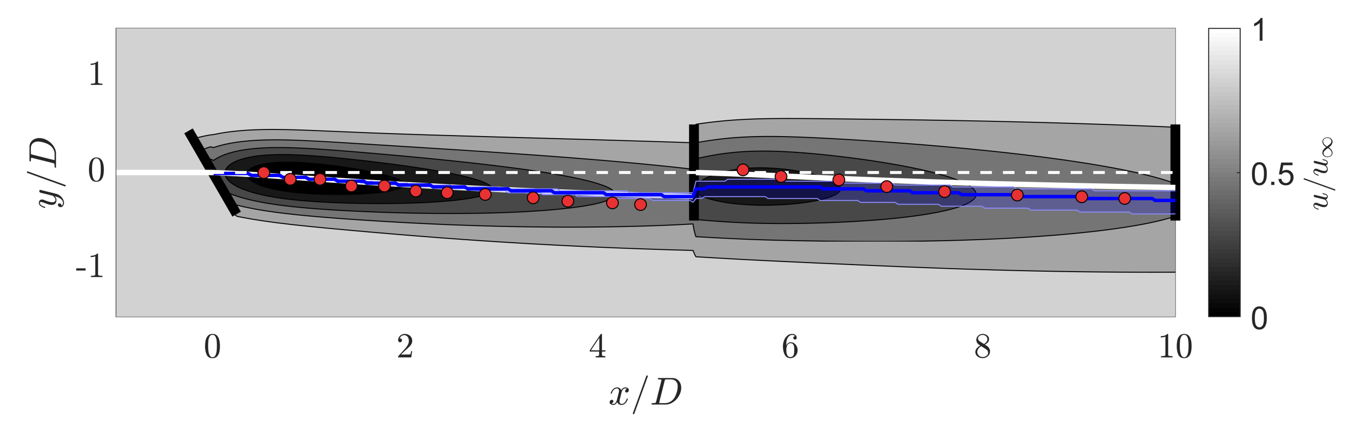
2.3. Two-Dimensional Secondary Steering Model

Yaw misaligned wind turbines induce a lateral velocity ($\delta v$) and a large-scale counter-rotating vortex pair (CVP) at the rotor extents in z (see, e.g., [31]). While the laterally induced momentum diffuses as a function of the downwind distance x, the lateral velocity may be $\delta v\ne 0$ at the location of the downwind turbines. Further, the CVP persists throughout the wake region as a function of x [31,41]. Fleming et al. (2018) [33] used LES to show that the CVP may persist for multiple rows of turbines downwind. As a result, the wake generated by a yaw aligned turbine operating in the wake of a yaw misaligned turbine will be deflected in the lateral direction as a function of x; this effect is termed secondary steering [33]. The development of a three-dimensional secondary steering model is on-going [42,43]; in this study, we develop a simple, analytical, two-dimensional secondary steering model to capture the effects of the non-vanishing $\delta v\left(x\right)$.

The transverse velocity is superposed using convective superposition [29] along the wake centerline to obtain the transverse velocity at the rotor of turbine j:

$$v_j^r=\delta v_{0,j}+\sum _i^{N_f}\frac{u_{i,j}^c}{U_j^c}\Delta v_{i,j},$$

(13)

where $\delta v_i$ is the transverse velocity deficit along turbine i’s wake centerline. The initial transverse velocity disturbance of turbine j according to ${\gamma }_j$ is $\delta v_{0,j}$. Equation (13) is included in the iterative procedure for the convective velocities (Section 2.2). Equation (13) can also be formulated using other superposition methodologies.

The initial transverse velocity disturbance is [35]:

$$\delta v_{0,j}=\frac{1}{4}{C}_{T,j}{u}_{0,i}{\cos }^2\left({\gamma }_j\right)\sin \left({\gamma }_j\right),$$

(14)

and the wake centerline transverse velocity is:

$$\delta v_i\left(x\right)=\frac{v_i^r}{d_{w,i}^2\left(x\right)}\frac{1}{2}\left[1+\mathrm{erf}\left(\frac{x}{\sqrt{2}D/2}\right)\right],$$

(15)

while the spanwise velocity is distributed as a presumed Gaussian function as with $du$, Equation (1). The spanwise velocity distribution trailing a yaw misaligned wind turbine exhibits asymmetries, which result in non-Gaussian profiles [31], and future work should investigate the two-dimensional lateral velocity profile. The rotor averaged lateral velocity deficit trailing turbine i at turbine j is:

$$\Delta v_{i,j}\left(x\right)=\frac{\sqrt{2\pi }\delta v_i\left(x\right)d_{w,i}\left(x\right)D}{16{\sigma }_{0,i}}\left[\mathrm{erf}\left(\frac{y_T+D/2-y_{c,i}\left(x\right)}{\sqrt{2}{\sigma }_{0,i}{d}_{w,i}\left(x\right)}\right)-\mathrm{erf}\left(\frac{y_T-D/2-y_{c,i}\left(x\right)}{\sqrt{2}{\sigma }_{0,i}{d}_{w,i}\left(x\right)}\right)\right].$$

(16)

For simplicity, the same proportionality constant for the presumed Gaussian wake ${\sigma }_0$ is used for the streamwise and lateral velocities, although future work could investigate this model selection. The two-dimensional secondary steering model proposed here does not introduce additional model parameters compared to the standard wake model presented in Section 2.2 with convective superposition.

The secondary steering methodology is compared to the wind tunnel experiments of Bastankhah and Porté-Agel (2019) [36] in Figure 1. Three turbines are considered with the leading turbine yaw misaligned at ${30}^{°}$, and the remaining turbines are yaw aligned. Further experimental configuration details can be found in Bastankhah and Porté-Agel (2019) [36]. The wake model parameters for Turbines 1 and 2 are set at $k_w=[0.08\pm 0.04,0.1\pm 0.04]$ and ${\sigma }_0=[0.25,0.35]$. Since the wake centroid depends on the wake model parameters, which are unknown for the experimental case, uncertainty in the wake model parameters is introduced into the selected values of $k_w$ as $\pm 0.04$. Two model wake center tracking methodologies are shown. The wake centroids of the individual wind turbine wakes are shown, as well as the wake centroid for the collective wake with convective superposition (see the wake superposition discussion in Section 2.2). The wake centroids for the collective wake from [36] are shown for comparison. While the accuracy of the model agreement with the experimental results of [36] depends on the wake model parameters, the reasonable parameters selected demonstrate the ability for the simple two-dimensional model proposed here to capture the trends of the secondary steering effect. The wake model parameters have a weak effect on the wake deflection associated with the leading wind turbine and a more significant influence on the collective wake centroid downwind of the second wind turbine.

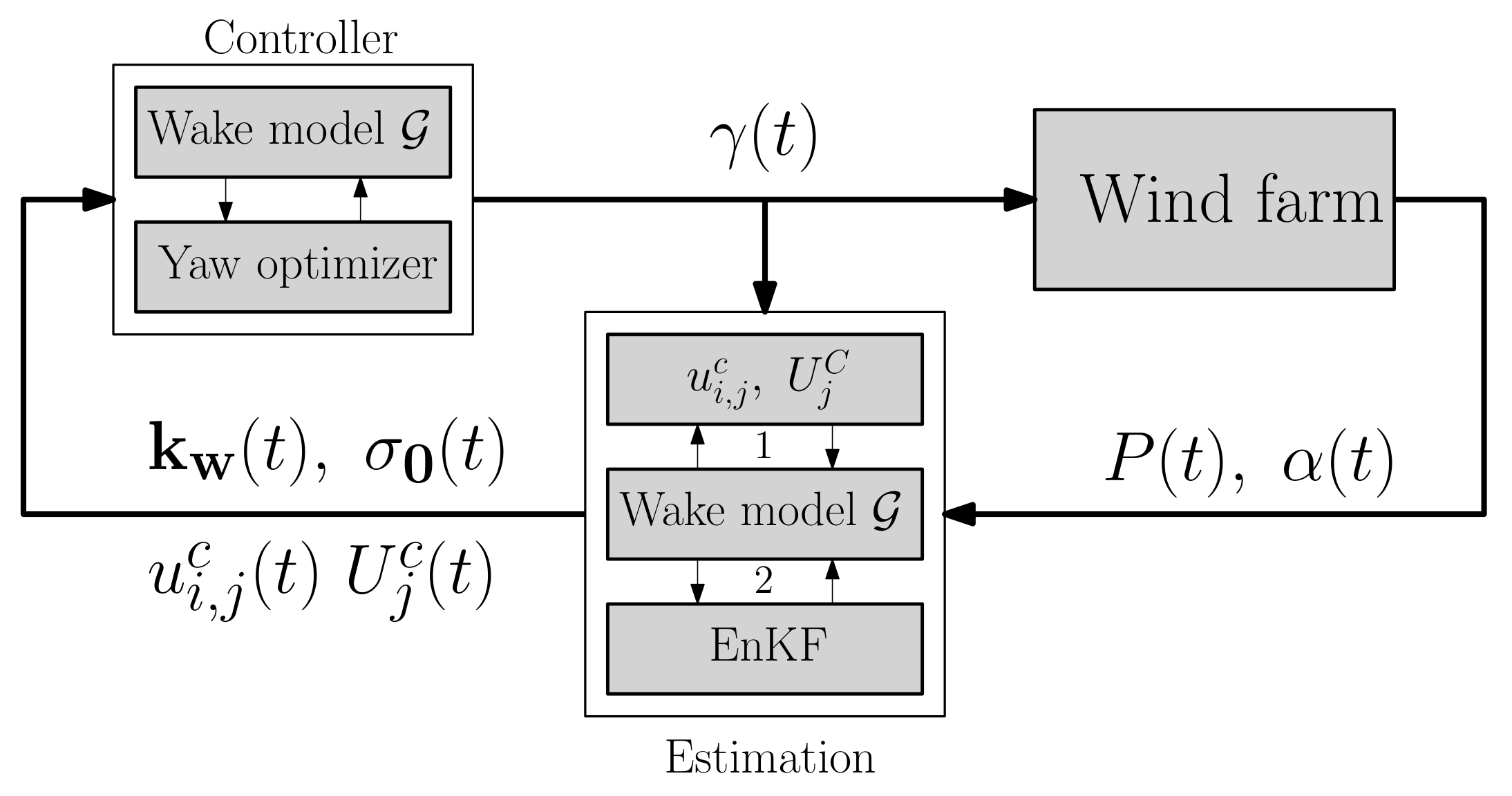
3. Closed-Loop Wake Steering Control

The effect of the wake superposition methodology and secondary steering model are tested in closed-loop control. The closed-loop wake steering controller selected in this study was developed by Howland et al., (2020) [10], and a schematic of the framework is shown in Figure 2. The wind farm power production data $P\left(t\right)$ (supervisory control and data acquisition (SCADA) data) and wind turbine measured wind direction $\alpha \left(t\right)$ are provided to the estimation algorithm. Collectively, the wake model can be written concisely as:

$$\widehat{P}=\mathcal{G}(X,Y,u_{\infty },\alpha ,\psi ),$$

(17)

a nonlinear function $\mathcal{G}$, which predicts the wind farm power production $\widehat{P}$ as a function of the wind farm layout in X and Y, the incident velocity $u_{\infty }$, and wind direction $\alpha$. The unknown wake model parameters are represented by $\psi =[k_{w,1},\dots ,k_{w,N_t-1},{\sigma }_{0,1},\dots ,{\sigma }_{0,N_t-1}]$, where $N_t$ is the number of wind turbines in the farm. In the first step of the estimation algorithm, the convection velocities are computed, if required for the wake superposition methodology (Equations (10) and (11)), for a given set of wake model parameters $\psi$. The optimal wake model parameters are then estimated by the ensemble Kalman filter (EnKF) [10,44]. The EnKF can be interpreted as a gradient-free optimizer to perform the inverse problem model parameter estimation for $\psi$ given wake model $\mathcal{G}$ and data P [45]. The model parameters and convection velocities are provided to the controller in which the wake model $\mathcal{G}$ and the yaw optimizer (Section 3.1) are used to calculate the model-optimal yaw misalignment angles for each wind turbine in the farm $\gamma \left(t\right)$. The objective function to be optimized in this study is the sum of the power productions over the turbines in the farm. In the present study, since the focus is on wake model physics, yaw actuation duty is not considered, although it has been shown to have a significant impact on the resulting wind farm power production under wake steering control and an influence on the optimal yaw misalignment update frequency [21].

Analytic Gradient-Based Yaw Set-Point Optimization

In order to efficiently optimize the yaw misalignment set-points for each wind turbine in the array, analytic gradient-based optimization is used [2]. These gradients are used to update the yaw misalignment set-points according to common gradient update algorithms (e.g., Adam optimization [46]). Analytic gradients are derived for the modified wake superposition methodologies discussed in Section 2.

The total gradient of the power with respect to the yaw angle of a given turbine i for linear wake superposition [26] is given as [2]:

$$\frac{\partial {\widehat{P}}_i}{\partial {\gamma }_i}=\frac{\partial {\widehat{P}}_i}{\partial C_{P,i}}\frac{\partial C_{P,i}}{\partial {\gamma }_i}+\frac{\partial {\widehat{P}}_i}{\partial C_{P,i}}\frac{\partial C_{P,i}}{\partial a_{p,i}}\frac{\partial a_{p,i}}{\partial C_{T,i}}\frac{\partial C_{T,i}}{\partial {\gamma }_i}.$$

(18)

The gradient of the power of a downstream turbine j with respect to the yawing decision of an upstream turbine i is:

$$\frac{\partial {\widehat{P}}_j}{\partial {\gamma }_i}=\frac{\partial {\widehat{P}}_j}{\partial u_{e,j}}\frac{\partial u_{e,j}}{\partial y_{c,i}}\frac{\partial y_{c,i}}{\partial {\gamma }_i}+\frac{\partial {\widehat{P}}_j}{\partial u_{e,j}}\frac{\partial u_{e,j}}{\partial a_i}\frac{\partial a_i}{\partial {\gamma }_i}.$$

(19)

With the modified linear wake superposition methodologies in Equations (7) and (12), additional terms arise for the gradient of the power of downstream turbines with respect to the yawing decisions of upwind turbines:

$$\frac{\partial {\widehat{P}}_j}{\partial {\gamma }_k}=\frac{\partial {\widehat{P}}_j}{\partial u_{e,j}}\frac{\partial u_{e,j}}{\partial u_{e,i}}\frac{\partial u_{e,i}}{\partial y_{c,k}}\frac{\partial y_{c,k}}{\partial {\gamma }_k}+\frac{\partial {\widehat{P}}_j}{\partial u_{e,j}}\frac{\partial u_{e,j}}{\partial u_{e,i}}\frac{\partial u_{e,i}}{\partial a_k}\frac{\partial a_k}{\partial {\gamma }_k},$$

(20)

where turbine k is upwind of turbine i, which is upwind of turbine j. With the secondary steering methodologies in Equation (13), additional terms arise for the gradient of the power of downstream turbines with respect to the yawing decisions of upwind turbines:

$$\frac{\partial {\widehat{P}}_j}{\partial {\gamma }_k}=\frac{\partial {\widehat{P}}_j}{\partial u_{e,j}}\frac{\partial u_{e,j}}{\partial y_{c,i}}\frac{\partial y_{c,i}}{\partial {\gamma }_k}$$

(21)

where turbine k is upwind of turbine i, which is upwind of turbine j.

The yaw misalignment angles are updated iteratively, until convergence, using the update step:

$${\gamma }^{(i+1)}={\gamma }^{\left(i\right)}+\alpha \frac{m_t}{\sqrt{v_t}},$$

(22)

where $m^{\left(i\right)}={\beta }_1{m}^{(i-1)}+(1-{\beta }_1)\frac{\partial \widehat{P}}{\partial \gamma }$ and $v^{\left(i\right)}={\beta }_2{v}^{(i-1)}+(1-{\beta }_2){\left(\frac{\partial \widehat{P}}{\partial \gamma }\right)}^2$. The hyperparameters ${\beta }_1=0.9$ and ${\beta }_2=0.999$ are set to typical values [46]. The superscript ${}^{\left(i\right)}$ denotes the step in the iterative optimization process.

The analytic gradients derived here are checked using numerical gradients for a model problem with three aligned turbines (see the SI Appendix in [2]). The numerical gradients are computed using second-order central finite differencing and are compared to the analytic gradients for the leading turbine and the last turbine downwind in Figure 3 for convective wake superposition (Equation (12)) with and without a secondary steering model. The comparison reveals close agreement between the numerical and analytic gradients for a variety of yaw misalignment angles implemented, validating the analytic derivation and algorithmic implementation of the gradient calculation.

4. Wake Steering Case Studies

In this section, the various wake model superposition methodologies are compared in their performance within closed-loop wake steering control. The secondary steering model proposed in Section 2.3 is also tested. In order to provide insights into the differences between the various wake model architectures, in Section 4.1, a six wind turbine test case is defined. Artificial wind farm power production data are defined for the test case, and the wake model parameters are estimated given the power data for the various superposition methodologies; the resulting optimal yaw misalignment angles and power production estimates are given. In Section 4.2, the wake models are tested in closed-loop control for a six wind turbine conventionally neutral atmospheric boundary layer (ABL) LES case.

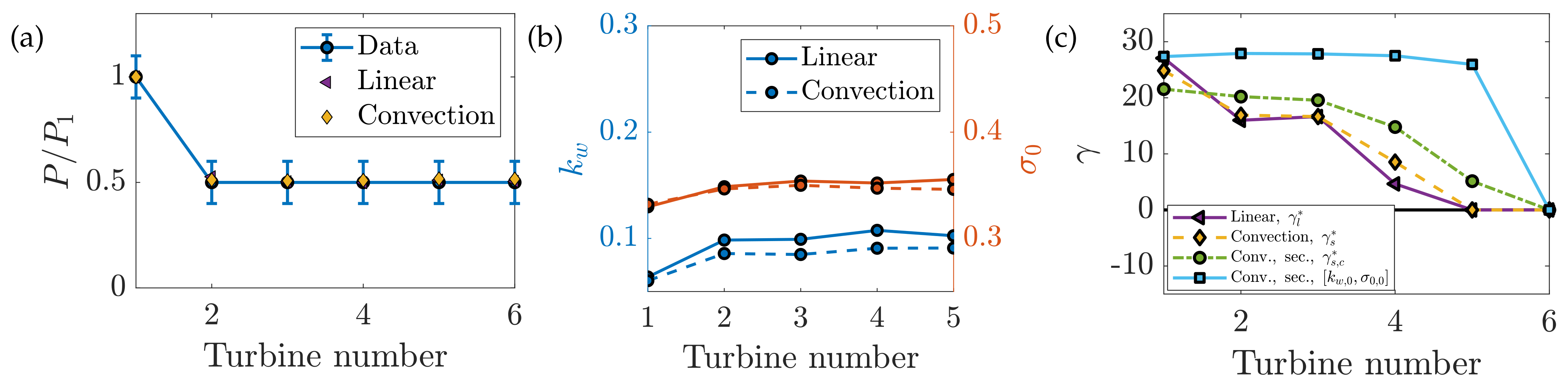
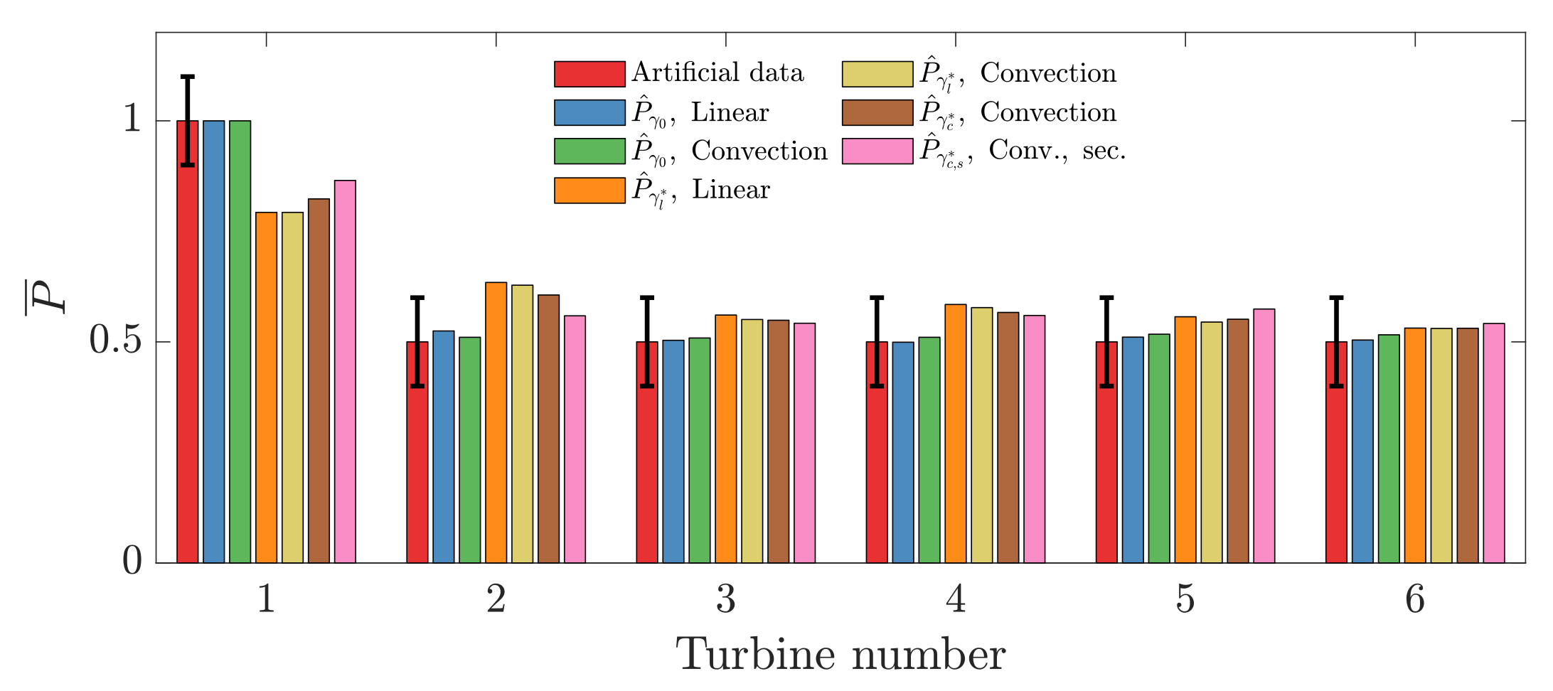
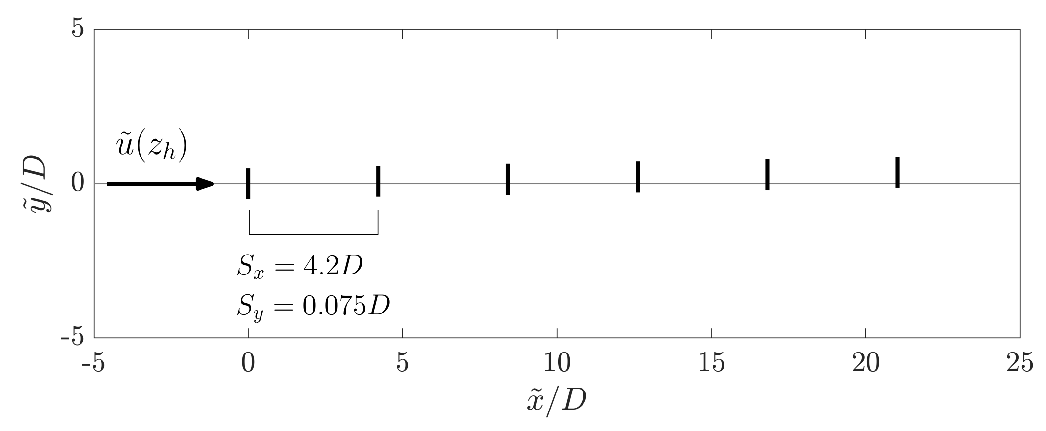
4.1. Six Turbine Test Case

Within the closed-loop wake steering algorithm described in Section 3, the model-optimal yaw misalignment angles, for fixed wind conditions, turbine details, and wake model physics, depend only on the wake model parameters. In turn, the wake model parameters are calculated based on the input wind farm power production data (see Figure 2). In order to elucidate the effects of the wake model wake deficit superposition method on closed-loop wake steering control, a six turbine test problem is defined. Provided fixed wind conditions, the turbine details and layout, and fixed wind farm power production data, differences in the wake model parameters and associated model-optimal yaw misalignment angles will be caused only by wake model physics modifications. Artificial data are designed for the test problem, and the results are revisited for LES of wind turbines operating in the conventionally neutral ABL in Section 4.2.

Six wind turbines are considered with a streamwise spacing of $S_x=8D$. The turbines are aligned in the lateral direction except for a small offset of $\epsilon ={10}^{-6}D$ applied to the lateral position of each successive turbine, such that the lateral positions are $Y_i=(i-1)·\epsilon ,$ for integer turbine labels $i=$ 1–6. The small offset $\epsilon$ is added to introduce asymmetry into the test problem such that $\gamma >0^{°}$ leads to improved performance compared to $\gamma <0^{°}$. While yaw misalignment has an asymmetric influence on the power production of wind turbine arrays due to wake rotation [38], Coriolis effects [47] and yaw misaligned turbine power production [18], the modeling of these effects is on-going and is not incorporated in the present wake model considered. Therefore, with direct turbine alignment, positive or negative yaw misalignment would lead to exactly equal power productions, and the $\epsilon$ offset reduces the possibility of two equal global maximum values. It is worth noting in practice that the probability of wind turbines to be aligned (to machine precision) in a field or LES application of wake steering is vanishingly small.

The artificial power production is shown in Figure 4a. A constant power production as a function of wind turbine row is often seen in experimental measurements of aligned wind turbine columns [36,48,49] as a result of convergence to a balance of turbulent mean kinetic energy transport and wind turbine energy sinks. The power data are prescribed Gaussian noise with zero mean and a standard deviation of $0.1P_1$. The power production estimations $\widehat{P}$ for the wake model with linear [26] and convective wake superposition [29] are shown in Figure 4a. Through the use of the EnKF wake model parameter estimation (see Figure 2), both linear and convective wake superposition are able to estimate the power production P with a low mean absolute error (MAE); the MAE is $0.0073P_1$ and $0.0105P_1$ for the linear and convective superposition methods, respectively. The resulting wake model parameters are provided in Figure 4b. For both linear and convective wake superposition, the wake model parameters $k_w$ and ${\sigma }_0$ weakly increase as a function of downwind row number. In general, increasing the $i$th turbine parameters $k_{w,i}$ or ${\sigma }_{0,i}$ decreases the magnitude of the individual $i$th wind turbine wake. For both linear and convective wake superposition, the increasing wake model parameters demonstrate that the individual wakes decrease their magnitude in order to fix the turbine power production as a function of the row number (Figure 4a). Secondary steering does not influence the wake model parameter estimation in this case since all wind turbines in the baseline control strategy corresponding to the artificial data are yaw aligned, and therefore, no lateral velocity is introduced into the wake model.

With the wake model parameters (Figure 4b) estimated from the EnKF provided with the power production shown in Figure 4a, yaw misalignment set-point optimization is performed. The yaw misalignment set-point optimization leverages analytic gradients, as discussed in Section 3.1. The optimization is run for linear wake superposition and convective wake superposition. Additionally, for convective wake superposition, the optimization is run separately with and without the secondary steering model. The resulting model-optimal yaw misalignment angle set-points are shown in Figure 4c. Finally, the optimal yaw misalignment angles for the convective wake superposition with secondary steering, but with no EnKF model parameter estimation are shown; the wake model parameters used are $k_w=0.08$ and ${\sigma }_0=0.25$ for each wind turbine in the array for the case without estimation.

The optimal yaw misalignment angles for linear ${\gamma }_l^{*}$ and convective ${\gamma }_c^{*}$ wake superposition are both qualitatively and quantitatively similar, with positive yaw misalignment angles, which decrease as a function of the turbine row number. With secondary steering incorporated, the yaw misalignment angle for the leading turbine is reduced, but the yaw misalignment for all other turbines is increased. For the case without estimation with fixed wake model parameters, the yaw misalignment values are approximately constant as a function of the turbine row. While the artificial data are not precisely representative of a physical wake steering case, and therefore there is no true global optimal set of yaw angles for reference, the differences arising between the various wake model architectures highlight a few key points. While the specific optimal yaw misalignment angles depend on the baseline power production and wind farm layout, there is a weak sensitivity of the optimal yaw set-points to the wake model superposition. There is a strong sensitivity of the optimal yaw set-points to the wake model parameters. With EnKF parameter estimation, convective superposition, and secondary steering incorporated, the model-optimal yaw set-points have a monotonic decrease as a function of the turbine row, which is similar to the reported experimental optimal yaw angles for a six turbine case case [36] (the yaw aligned baseline power production shown by [36] exhibited constant power production as a function of turbine row after Row 2, as do the artificial data in this section). The results of this case study suggest that the trend of decreasing optimal yaw misalignment magnitude as a function of turbine row is not specific to the secondary steering effect, but is more fundamental to the geometry and resulting power production associated with wind turbine interactions in a multi-row array.

The wake modeled power productions $\widehat{P}$ for the various wake steering experiments are shown in Figure 5. For reference, several additional results are shown. The power production associated with linear and convection wake superposition for yaw aligned operation $\gamma =0$ are shown with ${\widehat{P}}_{{\gamma }_0}$. Linear wake superposition predicts slightly smaller wake losses for Turbine 2 and slightly larger wake losses for Turbines 3, 4, 5, and 6. The optimal yaw misalignment angles for the linear superposition case are given by ${\gamma }_l^{*}$. These yaw angles, ${\gamma }_l^{*}$, are used to generate power production estimates for ${\widehat{P}}_{{\gamma }_l^{*}}$ for both linear and convection superposition. Again, the differences are very small, with linear superposition predicting slightly larger power for Turbines 2 through 6. The convective superposition with the associated convective superposition optimal yaw angles are shown with ${\widehat{P}}_{{\gamma }_c^{*}}$, and the convective superposition with secondary steering is shown with ${\widehat{P}}_{{\gamma }_{s,c}^{*}}$. The collective baseline power production is ${\sum }_i^{N_t}{\widehat{P}}_{i,{\gamma }_0}/P_{1,{\gamma }_0}=3.56$. The collective optimal power production predictions for the linear, convective, and convective with secondary steering are ${\sum }_i^{N_t}{\widehat{P}}_{i,{\gamma }_l^{*}}/P_{1,{\gamma }_0}=3.66$, ${\sum }_i^{N_t}{\widehat{P}}_{i,{\gamma }_s^{*}}/P_{1,{\gamma }_0}=3.63$, and ${\sum }_i^{N_t}{\widehat{P}}_{i,{\gamma }_{s,c}^{*}}/P_{1,{\gamma }_0}=3.64$. Overall, there are slight differences in the power production estimations $\widehat{P}$ between the various wake model physics cases, in addition to the optimal yaw angle differences mentioned previously, although all cases estimate power increases over baseline operation. Linear wake superposition estimates slightly more power increase due to wake steering than convective superposition. Secondary steering increases the magnitude of the estimate of power production improvement with wake steering control.

4.2. Conventionally Neutral ABL LES

In this section, the various wake model superposition methodologies are tested in large eddy simulations of a turbine array operating in the conventionally neutral ABL. The wind turbine array immersed in the LES ABL simulation is the surrogate for the wind farm block in Figure 2. During the simulation, closed-loop control is initiated with the control architecture described in Section 3. Within the wake model, a sub-component of the closed-loop control architecture (see Figure 2), the wake model superposition method, secondary steering model, and wake model parameter estimation methodologies are tested and compared to the baseline aligned control. In Section 4.2.1, the LES methodology and computational setup are introduced. The results and discussion are provided in Section 4.2.2.

4.2.1. Large Eddy Simulation Setup

Large eddy simulations of six turbines operating in the conventionally neutral ABL are performed using the open-source pseudo-spectral code PadéOps (https://github.com/FPAL-Stanford-University/PadeOps). LES simulations were previously performed with PadéOps to study planetary boundary layer turbulence [50], Coriolis effects [51], wind farm control [10], and multi-rotor wind turbines [52]. The conventionally neutral ABL is a representative planetary boundary layer wherein the background stratification has a zero lapse rate until the capping inversion and a stable free atmosphere [19,53,54]. Full details of the LES methodology were provided by [10], and relevant details are summarized here for completeness.

The LES is forced according to a geostrophic balance in the free atmosphere [55],

$$\frac{\partial P^G}{\partial x_i}=-\frac{2}{Ro}{\epsilon }_{ijk}{\mathsf{\Omega }}_j{G}_k,$$

(23)

where $P_G$ is the geostrophic pressure, G is the geostrophic wind vector, $\mathsf{\Omega }$ is Earth’s rotational vector, and $Ro=G_s/\omega L$ is the Rossby number, where $G_s$ is the geostrophic wind speed magnitude, $\omega$ is Earth’s angular velocity, and L is a relevant length scale. The horizontal directions are $x(i=1)$ and $y(i=2)$, and the wall-normal direction is $z(i=3)$. All simulations considered in this study prescribe a Froude number of $Fr=G_s/\sqrt{gL}=0.14$, where g is the gravitational acceleration, and a Rossby number based on the turbine rotor diameter of $R{o}_D=544$. The computational domain x-axis is aligned with the geostrophic wind speed vector such that $G=[G_s,0,0]$. All wind speeds are nondimensionalized by $G_s$. Wind turbines are modeled using the actuator disk model without rotation [56] and have diameters and hub heights of $D=126$ and $z_h=100$ m, respectively. The computational domain is $12\times 6\times 2.4$ km with $480\times 240\times 192$ grid points in the x, y, and z directions, respectively. The simulation is executed with a concurrent precursor methodology (see, e.g., [57,58]). The precursor simulation has the same domain setup and grid spacing with no turbine models included. The precursor outflow is provided to the primary domain as inflow conditions as a function of time to ensure realistic ABL turbulent inflow with appropriate time and length scales, but without the wake of the turbine array. The flow is initialized with perturbations in the potential temperature field and is run until quasi-statistical stationarity is reached; the closed-loop controller is then initiated (see [54] for a thorough discussion on ABL quasi-stationarity). Precursor simulation details were provided in [54].

Earth’s rotational vector is projected into a non-inertial Earth-fixed frame of reference such that $\mathsf{\Omega }=[0,\cos (\varphi ),\sin (\varphi \left)\right]$, where $\varphi$ is the latitude. The traditional approximation enforces the assumption that ${\mathsf{\Omega }}_2=0$ [55]. Non-traditional effects, such that ${\mathsf{\Omega }}_2\ne 0$, affect Ekman layer stability [59], wind turbine wakes [51], and the interaction of wind farms with the atmospheric boundary layer [54] and are therefore included in the present simulations. As a result of Coriolis effects, the wind direction depends on the height z, approximately following an Ekman spiral in the conventionally neutral ABL. The wind direction at the wind turbine hub height of $z_h=100$ m varies due to turbulence and inertial oscillations, but is approximately 14–19${}^{°}$, measured from the domain x-axis. Six model wind turbines are included in a column with an alignment offset by ${18}^{°}$ such that aerodynamic wake interactions persist between the turbines for the mean hub height inflow direction (Figure 6).

Upon quasi-statistical stationarity, the yaw control architecture is initialized. The mean wind farm statistics of power production and wind direction are averaged over a prescribed timescale T. The averaged LES model turbine power is normalized by $P_{1,{\gamma }_0}$, the actuator disk model power of the leading turbine given the existing primary LES flow field and $\gamma =0$. Future work may incorporate an additional adjacent reference turbine to calculate the normalizing power, which may be more robust given axial induction variations as a function of $\gamma$, but introduces uncertainty associated with wind field heterogeneity in finite time averages. The averaged quantities are provided to the parameter estimation algorithm to estimate the optimal model parameters over the previous time horizon of length T. The parameters are then provided to the optimizer, which estimates the optimal yaw misalignment given the wake model physics and wake model parameters corresponding to the averaged power production and wind direction provided by the LES wind farm. Within the conventionally neutral ABL, the mean states are approximately stationary except for inertial oscillations; however, significant high-frequency variations persist as a function of time due to turbulence. Therefore, the time step T in this study was selected to be 50 min (see the further discussion by [10]), to converge the statistics within each control update; within the turbulent, transient diurnal cycle ABL, the mean state of the wind conditions is constantly evolving, and a more rapid yaw misalignment update frequency would be required [21].

Case NA uses a baseline yaw aligned controller wherein at each control update (after time T), each wind turbine in the farm sets its nacelle position to equal its locally measured incident wind direction, therefore enforcing zero yaw misalignment aside from turbulent wind direction variations. The power production results of all cases are compared to Case NA as a function of time. The initialization and processor topology are fixed between the cases, and therefore, the differences that arise are only due to the differences in yaw misalignment. Upon wake steering initialization, the controller gathers baseline (yaw aligned) power production and wind direction data and averages over time T. For each case, the resulting power production and wind direction averages at the first control update step are identical to machine precision. The various wake steering controllers will then calculate differing model-optimal yaw misalignment angle set-points ${\gamma }_s^{*}$, and differences in LES power production will be correspondingly measured for the second control update step and beyond.

Case NL uses linear wake superposition Equation (8), [26]. The EnKF wake model parameter estimation is iterated for 2000 epochs to reduce the mean error associated with the wake model fit to the wind farm power data (as in ensemble Kalman inversion gradient-free optimization; seethe extensive discussion by [45]). Case NL1 also uses linear wake superposition, but does not iterate the EnKF parameter estimation (one epoch). As a result, the wake model power estimate $\widehat{P}$, which attempts to estimate P averaged over the previous window of time T, will have a higher calibration error, but the wake model parameters will be constrained more closely to their physics-based initialization prior belief (see the extensive discussion by [10]). Cases NC and NC1 are similar to NL and NL1 except convective wake superposition is used, Equation (12) [29]. Case NMS1 uses modified linear wake superposition Equation (7) with the secondary steering model incorporated, while Case NCS1 uses convective superposition and secondary steering. Finally, Cases NFCS1 and NFCS2 use convective superposition and secondary steering, but have fixed wake model parameters as a function of time (no EnKF parameter estimation). Case NFCS1 uses $k_w=0.1$ and ${\sigma }_0=0.25$ for each turbine in the array, and Case NFCS2 uses $k_w=0.1$ and ${\sigma }_0=0.35$.

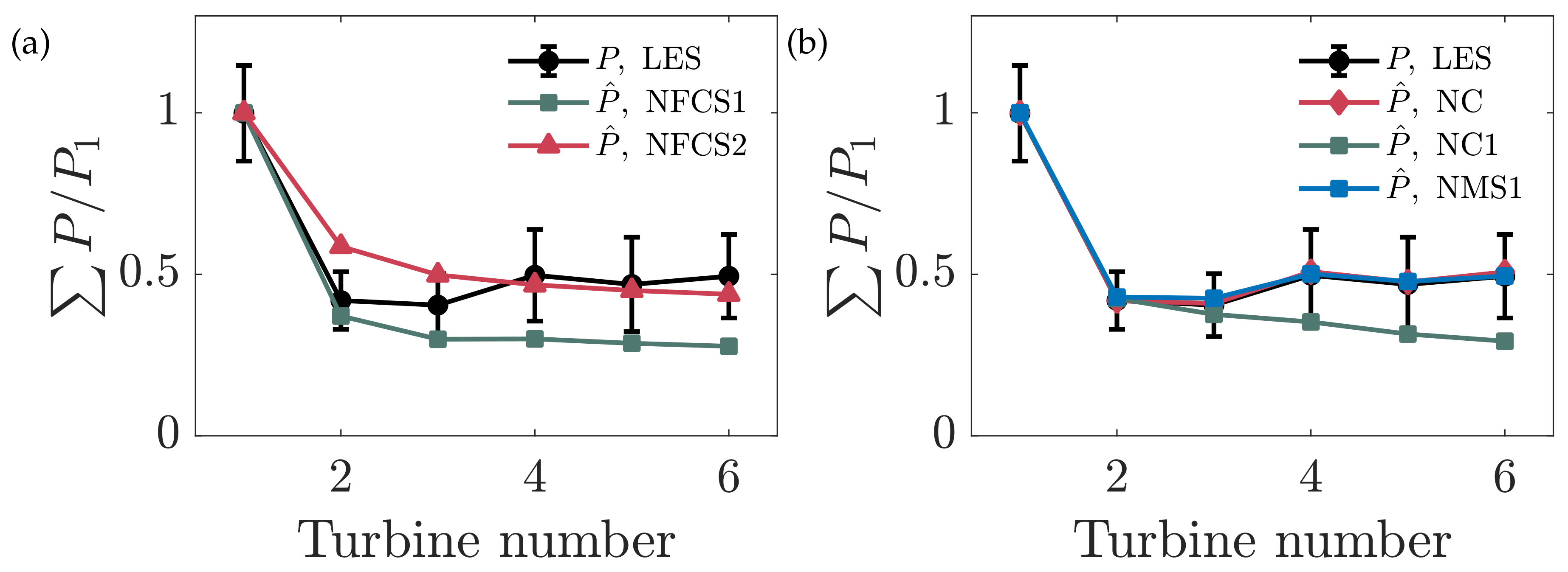
4.2.2. Large Eddy Simulation Results

The wake superposition and secondary steering methodologies are used in closed-loop control (Section 3) within the LES environment described in Section 4.2.1 in a variety of cases. Each case is run for 23 update time steps, each of length T, which is approximately 19 hours of physical wind farm operation in the conventionally neutral ABL. The results of each case are summarized in

Table 1. Wake model superposition LES experiments. The cases are defined in Section 4.2.1. The power production percent gains are provided with respect to Case NA. The array power production sums are normalized by the leading turbine power production in yaw aligned control $P_{\mathrm{baseline},1}$. Cases NFCS1 and NFCS2 have fixed wake model parameters and do not execute EnKF parameter estimation.

Case	Steering	Superposition	Epochs	$\frac{\sum \mathit{P}-\sum {\mathit{P}}_{\mathbf{aligned}}}{\sum {\mathit{P}}_{\mathbf{aligned}}}(\%)$	$\overline{\sum \mathit{P}}\pm \mathbf{STD}(\sum \mathit{P})$
	Wind turbine column alignment ${18}^{°}$
NA	-	-	-	-	$3.04\pm 0.11$
NL	✓	Linear	2000	$5.0\%$	$3.18\pm 0.13$
NL1	✓	Linear	1	$5.7\%$	$3.20\pm 0.11$
NC	✓	Convective	2000	$6.6\%$	$3.23\pm 0.11$
NC1	✓	Convective	1	$7.2\%$	$3.24\pm 0.10$
NMS1	✓	Mod., Sec.	1	$7.5\%$	$3.26\pm 0.11$
NCS1	✓	Conv., Sec.	1	$7.7\%$	$3.26\pm 0.12$
NFCS1	✓	Conv., Sec.	0	$7.8\%$	$3.26\pm 0.11$
NFCS2	✓	Conv., Sec.	0	$6.4\%$	$3.22\pm 0.13$

. The time averaged wind turbine array power production for each case is shown in Figure 7a. The averaged power for each case is compared to Case NL1, the linear superposition case with one EnKF estimation epoch; cases with statistically significantly more power than Case NL1, as tested by a one-sided two-sample Kolmogorov–Smirnov test at a $5\%$ significance level, are indicated in Figure 7a. The mean absolute errors (MAE) of the wake model predictions for the power production given the yaw misalignment set-point ${\gamma }_s^{*}$ are shown in Figure 7b. The wake model predictions ${\widehat{P}}_t$ of time step t are compared to the LES power production $P_{t+1}$ results of $t+1$. The modified linear and convective wake superposition models underpredict the realized LES power production under wake steering control for every time step, whereas the linear wake superposition Cases NL and NL1 overpredict the power in $60\%$ and $10\%$ of the control update steps, respectively. The time averaged power production and yaw misalignment as a function of the turbine number in the array are shown in Figure 8a,b, respectively.

All cases under wake steering control produce significantly more power than baseline yaw aligned control in this conventionally neutral LES environment. Cases with EnKF epochs greater than one (NL and NC) have reduced performance compared to a single parameter estimation step (NL1 and NC1). The wake steering strategy in linear wake superposition is more sensitive to the wake model parameters than the convective superposition, as shown in Figure 8b. The yaw misalignments for Cases NC and NC1 are similar, whereas ${\gamma }_s^{*}$ for Cases NL and NL1 are significantly different. The inverse problem to compute the optimal model parameters for the convective superposition is more complex as a result of the iterative convective velocity calculation, leading to larger variations in the resulting wake model parameters for linear superposition than for convective.

While increasing the number of EnKF epochs reduces the training MAE for all cases (not shown for brevity), it increases the predictive MAE for linear superposition, but reduces the predictive MAE for convective superposition. The power production training power estimates $\widehat{P}$ compared to the LES power P for convective and modified linear superposition are shown in Figure 9. Case NC, with a larger number of EnKF epochs, is able to train to estimate P with low MAE. However, Case NC1, with only one EnKF epoch, has significant training MAE compared to Case NC. Finally, Case NMS1, with only one EnKF epoch, but modified linear superposition instead of convective superposition, has low training MAE. Together, the results suggest that the nonlinear, iterative calculation of the convective velocities, the only difference between the convective and modified linear wake superposition methodologies, introduces complexity into the model parameter estimation inverse problem and therefore generates larger training MAE.

As discussed by Howland et al., (2020) [10], the hyperparameters of the wake model variances and parameter estimation epochs establish parameter constraints on $k_w$ and ${\sigma }_0$. With a larger number of parameter estimation epochs, the training error (fitting error to the previous control update step power measurements) is reduced; however, this behavior exhibits overfitting and potentially correcting for model bias. Instead, with the prescribed wake model parameter variances and one estimation epoch, the wake model parameter modifications are constrained by the prior belief of the parameters, therefore imposing a minimum threshold of performance for the physics-based wake model (see also the discussion by Schreiber et al., (2020) [60]). As such, all comparisons for the remainder of this discussion will be made to cases with a single parameter estimation step.

In a wake steering application, the wake model parameters are unknown a priori, and tabulated physics-based wake model parameters introduce significant model predictive bias, as shown in Figure 7b (see also [10]). Cases NFCS1 and NFCS2 prescribe two different cases of fixed wake model parameters within the expected parameter range and utilize convective wake superposition. Both cases prescribe $k_w=0.1$ for each turbine, and Case NFCS1 prescribes ${\sigma }_0=0.25$, while Case NFCS2 prescribes ${\sigma }_0=0.35$. Reducing ${\sigma }_0$ increases the magnitude of the predicted wake losses for downwind turbines. As a result, the baseline model predictions for yaw aligned operation will have significantly higher wake losses in Case NFCS1, and the corresponding model-optimal yaw misalignment values in Case NFCS1 are significantly larger than Case NFCS2 (see Figure 8b). The turbine array power production results are compared to Case NL1. Case NFCS1 has statistically significantly higher power production than Case NL1, while Case NFCS2 does not. The wake model power production estimates $\widehat{P}$ for Cases NFCS1 and NFCS2 are compared to the LES power production P in Figure 9a. The prescribed wake model parameters in Case NFCS1 generally overpredict the wake losses, while Case NFCS2 underpredicts the losses. Both cases capture the qualitative wake power deficit profile shape with power production decreasing significantly from Turbine 1 to 2 and then remaining approximately constant thereafter. As a result of the wake model parameters, the wake steering approach in Case NFCS1 is aggressive, with larger values of yaw misalignment, while Case NFCS2 is conservative. Case NFCS1 performs similarly to Case NCS1, which leverages EnKF, while Case NFCS2 performs statistically significantly worse. These results suggest that the EnKF model parameter estimation reduces predictive wake model error and may lead to enhanced wake steering performance. Although some a priori wake model parameter estimates may be sufficient to realize power production increases, as in Case NFCS1, these potential increases come with significant uncertainty and predictive error (see Figure 7b). As a result, site- and time-specific wake model parameter estimation is suggested as a mechanism to reduce the uncertainty associated with wake steering power production increase forecasts.

The three wake deficit superposition methodologies are tested in closed-loop control in LES. Both modified linear superposition (Case NMS1) and convective superposition (Case NCS1) produce significantly more power than linear wake superposition (Case NL1). However, Case NCS1 is not significantly better than Case NMS1. Modified linear superposition (Case NMS1) has slightly larger averaged yaw set-points than convective superposition (Case NCS1). The predictive MAE associated with NMS1 is less than Case NCS1. The higher predictive MAE associated with NCS1 is likely related to the additional complexity introduced into the inverse problem of parameter estimation (see Figure 9b).

The secondary steering model proposed in Section 2.3 is also tested in LES between Cases NC1 and NCS1, where the only architectural difference between the two simulations is that the wake model in Case NCS1 includes secondary steering effects. The inclusion of the secondary steering model increases the resulting power production and reduces the predictive MAE, although the effect on the power production is not statistically significant in this case. Interestingly, in this partial wake scenario (Figure 6), the inclusion of secondary steering results in an increase in the magnitude of the yaw misalignment set-points ${\gamma }_s^{*}$, except for Turbine 5. Further, there is not a noticeable decrease in the magnitude of the yaw misalignment angles as a function of the turbine row, again except for Turbine 5, which occurs in the directly aligned wind turbine column case (see the discussion by King et al. (2020) [42]). Instead, in the present case with the prescribed yaw misalignments shown in Figure 8b, the power production of the downwind turbines increases, especially for Turbine 6. This would potentially not occur for a larger wind farm scenario where deep array effects may be significant [61]. Future work should investigate the statistical significance of a fully three-dimensional secondary steering model.

5. Conclusions

This paper investigates the effects of wake velocity deficit superposition methodologies, wake model parameter estimation, and secondary steering models in the context of closed-loop wake steering control. An analytic formulation of the lifting line model [2,35] is derived for arbitrary wake velocity deficit superposition methodologies and the associated analytic gradients are presented. A simple two-dimensional secondary steering model is developed and validated against previously published experimental results given wake model parameter uncertainty. The various wake model superposition methodologies are tested in closed-loop control of a six wind turbine array embedded in a large eddy simulation of a conventionally neutral atmospheric boundary layer with Coriolis effects included. The main conclusions are:

• Modified linear [28] and convective [29] superposition methodologies produce statistically significantly higher power in the present case than linear superposition [26].
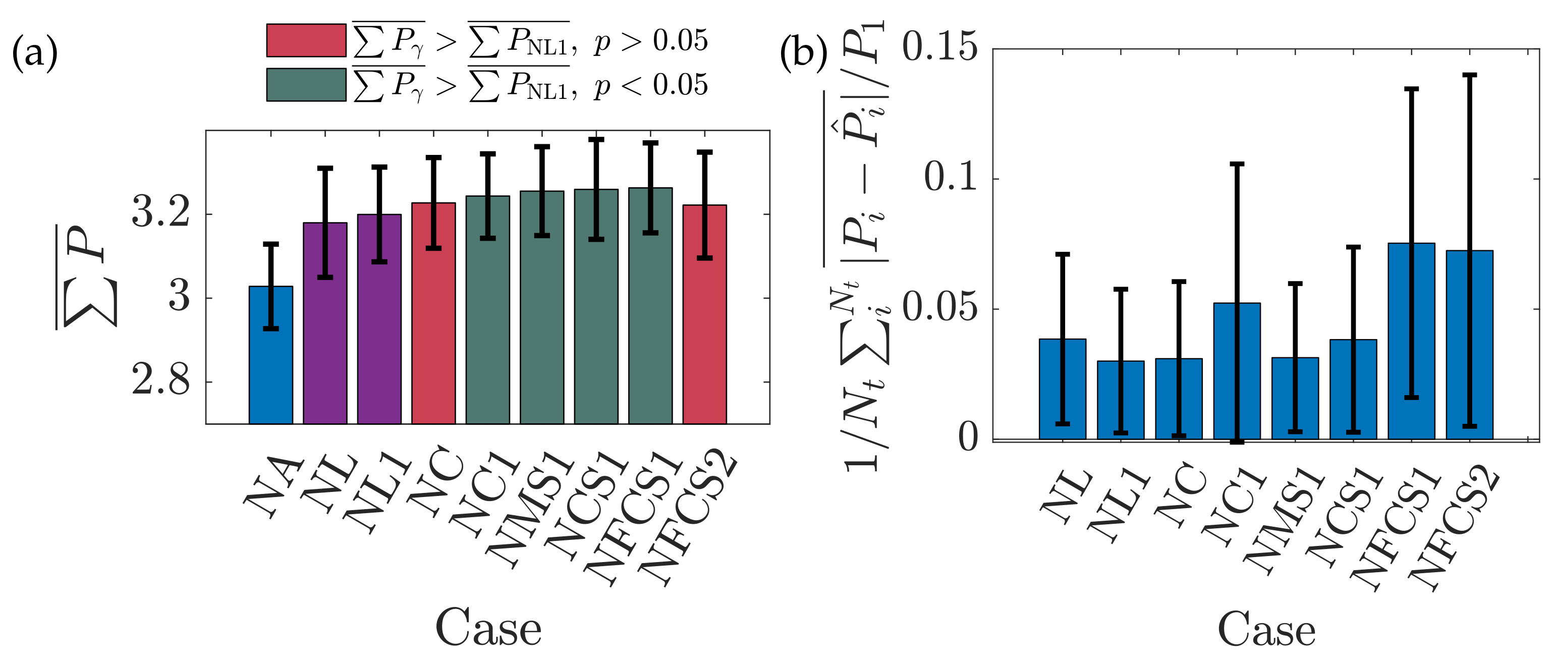
• Convective superposition [29] leads to the larger power gain over the baseline control than modified linear superposition, although it was not significantly higher.
• The nonlinear, iterative procedure required to compute the convective velocities in the convective wake superposition methodology results in increased predictive error due to additional complexity in the model parameter inverse problem, suggesting that the optimal parameter estimation requires more investigation for convective superposition.
• The proposed secondary steering model increases the power production and reduces predictive MAE, but does not have a statistically significant impact on the closed-loop wake steering case presented.

A major outstanding issue within analytic wake models is model predictive bias. While the ensemble Kalman filter parameter estimation significantly reduces the mean absolute error associated with the wake model predictions, model bias remains due to the nature of the simplified wake model. With the two-dimensional secondary steering model presented in this study, the modified linear and convective wake superposition methods underpredict the LES power given wake steering operation for all control update steps, suggesting the influence of three-dimensional curled wake effects [31] and wind speed and direction shear effects [62]. Future work should consider the novel hybrid RANS/analytic wake model developed by Martínez-Tossas et al., (2020) [43], which reduces the predictive bias compared analytic wake models by capturing the three-dimensional curled wake deformation [31]. Future work should also incorporate yaw actuation duty into the closed-loop yaw misalignment set-point optimization framework [21].

References

1. Barthelmie, R.J.; Hansen, K.; Frandsen, S.T.; Rathmann, O.; Schepers, J.; Schlez, W.; Phillips, J.; Rados, K.; Zervos, A.; Politis, E. Modelling and measuring flow and wind turbine wakes in large wind farms offshore. Wind Energy 2009, 12, 431–444. [Google Scholar] [CrossRef]
2. Howland, M.F.; Lele, S.K.; Dabiri, J.O. Wind farm power optimization through wake steering. Proc. Natl. Acad. Sci. USA 2019, 116, 14495–14500. [Google Scholar] [CrossRef] [PubMed] [Green Version]
3. Stevens, R.J.; Hobbs, B.F.; Ramos, A.; Meneveau, C. Combining economic and fluid dynamic models to determine the optimal spacing in very large wind farms. Wind Energy 2017, 20, 465–477. [Google Scholar] [CrossRef]
4. Fleming, P.; Gebraad, P.M.; Lee, S.; van Wingerden, J.W.; Johnson, K.; Churchfield, M.; Michalakes, J.; Spalart, P.; Moriarty, P. Simulation comparison of wake mitigation control strategies for a two-turbine case. Wind Energy 2015, 18, 2135–2143. [Google Scholar] [CrossRef]
5. Gebraad, P.; Thomas, J.J.; Ning, A.; Fleming, P.; Dykes, K. Maximization of the annual energy production of wind power plants by optimization of layout and yaw-based wake control. Wind Energy 2017, 20, 97–107. [Google Scholar] [CrossRef] [Green Version]
6. Kheirabadi, A.C.; Nagamune, R. A quantitative review of wind farm control with the objective of wind farm power maximization. J. Wind Eng. Ind. Aerodyn. 2019, 192, 45–73. [Google Scholar] [CrossRef]
7. Jiménez, Á.; Crespo, A.; Migoya, E. Application of a LES technique to characterize the wake deflection of a wind turbine in yaw. Wind Energy 2010, 13, 559–572. [Google Scholar] [CrossRef]
8. Fleming, P.; King, J.; Dykes, K.; Simley, E.; Roadman, J.; Scholbrock, A.; Murphy, P.; Lundquist, J.K.; Moriarty, P.; Fleming, K.; et al. Initial results from a field campaign of wake steering applied at a commercial wind farm–Part 1. Wind Energy Sci. 2019, 4, 273–285. [Google Scholar] [CrossRef] [Green Version]
9. Fleming, P.; Annoni, J.; Shah, J.J.; Wang, L.; Ananthan, S.; Zhang, Z.; Hutchings, K.; Wang, P.; Chen, W.; Chen, L. Field test of wake steering at an offshore wind farm. Wind Energy Sci. 2017, 2, 229–239. [Google Scholar] [CrossRef] [Green Version]
10. Howland, M.F.; Ghate, A.S.; Lele, S.K.; Dabiri, J.O. Optimal closed-loop wake steering–Part 1: Conventionally neutral atmospheric boundary layer conditions. Wind Energy Sci. 2020, 5, 1315–1338. [Google Scholar] [CrossRef]
11. Rott, A.; Doekemeijer, B.; Seifert, J.K.; Wingerden, J.W.V.; Kühn, M. Robust active wake control in consideration of wind direction variability and uncertainty. Wind Energy Sci. 2018, 3, 869–882. [Google Scholar] [CrossRef] [Green Version]
12. Quick, J.; Annoni, J.; King, R.; Dykes, K.; Fleming, P.; Ning, A. Optimization under uncertainty for wake steering strategies. J. Phys. Conf. Ser. 2017, 854, 012036. [Google Scholar] [CrossRef]
13. Simley, E.; Fleming, P.; King, J. Design and analysis of a wake steering controller with wind direction variability. Wind Energy Sci. 2020, 5, 451–468. [Google Scholar] [CrossRef] [Green Version]
14. Staffell, I.; Green, R. How does wind farm performance decline with age? Renew. Energy 2014, 66, 775–786. [Google Scholar] [CrossRef] [Green Version]
15. Wharton, S.; Lundquist, J.K. Atmospheric stability affects wind turbine power collection. Environ. Res. Lett. 2012, 7, 014005. [Google Scholar] [CrossRef]
16. Ghate, A.S.; Ghaisas, N.; Lele, S.K.; Towne, A. Interaction of small scale homogenenous isotropic turbulence with an actuator disk. In Proceedings of the 2018 Wind Energy Symposium, Kissimmee, FL, USA, 8–12 January 2018; p. 0753. [Google Scholar]
17. Sanchez Gomez, M.; Lundquist, J.K. The effect of wind direction shear on turbine performance in a wind farm in central Iowa. Wind Energy Sci. 2020, 5, 125–139. [Google Scholar] [CrossRef] [Green Version]
18. Howland, M.F.; Gonzalez, C.M.; Martinez, J.J.P.; Quesada, J.B.; Larranaga, F.P.; Yadav, N.K.; Chawla, J.S.; Dabiri, J.O. Influence of atmospheric conditions on the power production of utility-scale wind turbines in yaw misalignment. J. Renew. Sustain. Energy 2020, 12, 063307. [Google Scholar] [CrossRef]
19. Allaerts, D.; Meyers, J. Large eddy simulation of a large wind-turbine array in a conventionally neutral atmospheric boundary layer. Phys. Fluids 2015, 27, 065108. [Google Scholar] [CrossRef] [Green Version]
20. Ciri, U.; Rotea, M.A.; Leonardi, S. Model-free control of wind farms: A comparative study between individual and coordinated extremum seeking. Renew. Energy 2017, 113, 1033–1045. [Google Scholar] [CrossRef]
21. Kanev, S. Dynamic wake steering and its impact on wind farm power production and yaw actuator duty. Renew. Energy 2020, 146, 9–15. [Google Scholar] [CrossRef] [Green Version]
22. Doekemeijer, B.M.; van der Hoek, D.; van Wingerden, J.W. Closed-loop model-based wind farm control using FLORIS under time-varying inflow conditions. Renew. Energy 2020, 156, 719–730. [Google Scholar] [CrossRef]
23. Howland, M.F.; Dabiri, J.O. Wind farm modeling with interpretable physics-informed machine learning. Energies 2019, 12, 2716. [Google Scholar] [CrossRef] [Green Version]
24. Stevens, R.J.; Gayme, D.F.; Meneveau, C. Coupled wake boundary layer model of wind-farms. J. Renew. Sustain. Energy 2015, 7, 023115. [Google Scholar] [CrossRef] [Green Version]
25. Archer, C.L.; Vasel-Be-Hagh, A.; Yan, C.; Wu, S.; Pan, Y.; Brodie, J.F.; Maguire, A.E. Review and evaluation of wake loss models for wind energy applications. Appl. Energy 2018, 226, 1187–1207. [Google Scholar] [CrossRef]
26. Lissaman, P. Energy effectiveness of arbitrary arrays of wind turbines. J. Energy 1979, 3, 323–328. [Google Scholar] [CrossRef]
27. Katic, I.; Højstrup, J.; Jensen, N.O. A simple model for cluster efficiency. In Proceedings of the European Wind Energy Association Conference and Exhibition, Rome, Italy, 6–8 October 1986. [Google Scholar]
28. Niayifar, A.; Porté-Agel, F. Analytical modeling of wind farms: A new approach for power prediction. Energies 2016, 9, 741. [Google Scholar] [CrossRef] [Green Version]
29. Zong, H.; Porté-Agel, F. A momentum-conserving wake superposition method for wind farm power prediction. J. Fluid Mech. 2020, 889, A8. [Google Scholar] [CrossRef]
30. Medici, D.; Alfredsson, P. Measurements on a wind turbine wake: 3D effects and bluff body vortex shedding. Wind Energy: Int. J. Prog. Appl. Wind Power Convers. Technol. 2006, 9, 219–236. [Google Scholar] [CrossRef]
31. Howland, M.F.; Bossuyt, J.; Martínez-Tossas, L.A.; Meyers, J.; Meneveau, C. Wake structure in actuator disk models of wind turbines in yaw under uniform inflow conditions. J. Renew. Sustain. Energy 2016, 8, 043301. [Google Scholar] [CrossRef] [Green Version]
32. Bastankhah, M.; Porté-Agel, F. Experimental and theoretical study of wind turbine wakes in yawed conditions. J. Fluid Mech. 2016, 806, 506–541. [Google Scholar] [CrossRef]
33. Fleming, P.; Annoni, J.; Churchfield, M.; Martinez-Tossas, L.A.; Gruchalla, K.; Lawson, M.; Moriarty, P. A simulation study demonstrating the importance of large-scale trailing vortices in wake steering. Wind Energy Sci. 2018, 3, 243–255. [Google Scholar] [CrossRef] [Green Version]
34. Bastankhah, M.; Porté-Agel, F. A new analytical model for wind-turbine wakes. Renew. Energy 2014, 70, 116–123. [Google Scholar] [CrossRef]
35. Shapiro, C.R.; Gayme, D.F.; Meneveau, C. Modelling yawed wind turbine wakes: A lifting line approach. J. Fluid Mech. 2018, 841. [Google Scholar] [CrossRef] [Green Version]
36. Bastankhah, M.; Porté-Agel, F. Wind farm power optimization via yaw angle control: A wind tunnel study. J. Renew. Sustain. Energy 2019, 11, 023301. [Google Scholar] [CrossRef] [Green Version]
37. Medici, D. Experimental Studies of Wind Turbine Wakes: Power Optimisation and Meandering. Ph.D. Thesis, KTH Royal Institute of Technology, Stockholm, Sweden, 2005. [Google Scholar]
38. Gebraad, P.; Teeuwisse, F.; Van Wingerden, J.; Fleming, P.A.; Ruben, S.; Marden, J.; Pao, L. Wind plant power optimization through yaw control using a parametric model for wake effects—A CFD simulation study. Wind Energy 2016, 19, 95–114. [Google Scholar] [CrossRef]
39. Martínez-Tossas, L.A.; Churchfield, M.J.; Leonardi, S. Large eddy simulations of the flow past wind turbines: Actuator line and disk modeling. Wind Energy 2015, 18, 1047–1060. [Google Scholar] [CrossRef]
40. Yang, X.; Sotiropoulos, F. A new class of actuator surface models for wind turbines. Wind Energy 2018, 21, 285–302. [Google Scholar] [CrossRef] [Green Version]
41. Martinez-Tossas, L.; Howland, M.; Meneveau, C. Large eddy simulation of wind turbine wakes with yaw effects. In Proceedings of the 68th Annual Meeting of the APS Division of Fluid Dynamics (APS DFD GFM), Boston, MA, USA, 22–24 November 2015. [Google Scholar]
42. King, J.; Fleming, P.; King, R.; Martínez-Tossas, L.A.; Bay, C.J.; Mudafort, R.; Simley, E. Controls-Oriented Model for Secondary Effects of Wake Steering. Wind Energy Sci. Discuss. 2020, 1–22. [Google Scholar] [CrossRef] [Green Version]
43. Martínez-Tossas, L.A.; King, J.; Quon, E.; Bay, C.J.; Mudafort, R.; Hamilton, N.; Fleming, P. The curled wake model: A three-dimensional and extremely fast steady-state wake solver for wind plant flows. Wind Energy Sci. Discuss. 2020, 1–16. [Google Scholar] [CrossRef]
44. Evensen, G. The ensemble Kalman filter: Theoretical formulation and practical implementation. Ocean Dyn. 2003, 53, 343–367. [Google Scholar] [CrossRef]
45. Iglesias, M.A.; Law, K.J.; Stuart, A.M. Ensemble Kalman methods for inverse problems. Inverse Probl. 2013, 29, 045001. [Google Scholar] [CrossRef]
46. Kingma, D.P.; Ba, J. Adam: A method for stochastic optimization. arXiv 2014, arXiv:1412.6980. [Google Scholar]
47. Archer, C.L.; Vasel-Be-Hagh, A. Wake steering via yaw control in multi-turbine wind farms: Recommendations based on large-eddy simulation. Sustain. Energy Technol. Assess. 2019, 33, 34–43. [Google Scholar] [CrossRef]
48. Barthelmie, R.J.; Frandsen, S.T.; Nielsen, M.; Pryor, S.; Rethore, P.E.; Jørgensen, H.E. Modelling and measurements of power losses and turbulence intensity in wind turbine wakes at Middelgrunden offshore wind farm. Wind Energy 2007, 10, 517–528. [Google Scholar] [CrossRef]
49. Bossuyt, J.; Howland, M.F.; Meneveau, C.; Meyers, J. Measurement of unsteady loading and power output variability in a micro wind farm model in a wind tunnel. Exp. Fluids 2017, 58, 1. [Google Scholar] [CrossRef] [Green Version]
50. Ghate, A.S.; Lele, S.K. Subfilter-scale enrichment of planetary boundary layer large eddy simulation using discrete Fourier–Gabor modes. J. Fluid Mech. 2017, 819, 494–539. [Google Scholar] [CrossRef]
51. Howland, M.F.; Ghate, A.S.; Lele, S.K. Influence of the horizontal component of Earth’s rotation on wind turbine wakes. J. Phys. Conf. Ser. 2018, 1037, 072003. [Google Scholar] [CrossRef] [Green Version]
52. Ghaisas, N.S.; Ghate, A.S.; Lele, S.K. Effect of tip spacing, thrust coefficient and turbine spacing in multi-rotor wind turbines and farms. Wind Energy Sci. 2020, 5, 51–72. [Google Scholar] [CrossRef] [Green Version]
53. Zilitinkevich, S.; Esau, I. On integral measures of the neutral barotropic planetary boundary layer. Bound. Layer Meteorol. 2002, 104, 371–379. [Google Scholar] [CrossRef]
54. Howland, M.F.; Ghate, A.S.; Lele, S.K. Influence of the geostrophic wind direction on the atmospheric boundary layer flow. J. Fluid Mech. 2020, 883, A39. [Google Scholar] [CrossRef]
55. Wyngaard, J.C. Turbulence in the Atmosphere; Cambridge University Press: Cambridge, UK, 2010. [Google Scholar]
56. Calaf, M.; Meneveau, C.; Meyers, J. Large eddy simulation study of fully developed wind-turbine array boundary layers. Phys. Fluids 2010, 22, 015110. [Google Scholar] [CrossRef] [Green Version]
57. Munters, W.; Meneveau, C.; Meyers, J. Turbulent inflow precursor method with time-varying direction for large-eddy simulations and applications to wind farms. Bound. Layer Meteorol. 2016, 159, 305–328. [Google Scholar] [CrossRef] [Green Version]
58. Howland, M.F.; Ghate, A.S.; Lele, S.K. Coriolis effects within and trailing a large finite wind farm. In Proceedings of the AIAA Scitech 2020 Forum, Orlando, FL, USA, 6–10 January 2020; p. 0994. [Google Scholar]
59. Leibovich, S.; Lele, S. The influence of the horizontal component of Earth’s angular velocity on the instability of the Ekman layer. J. Fluid Mech. 1985, 150, 41–87. [Google Scholar] [CrossRef]
60. Schreiber, J.; Bottasso, C.L.; Salbert, B.; Campagnolo, F. Improving wind farm flow models by learning from operational data. Wind Energy Sci. Discuss. 2019. [Google Scholar] [CrossRef]
61. Barthelmie, R.J.; Jensen, L. Evaluation of wind farm efficiency and wind turbine wakes at the Nysted offshore wind farm. Wind Energy 2010, 13, 573–586. [Google Scholar] [CrossRef]
62. Abkar, M.; Sørensen, J.N.; Porté-Agel, F. An analytical model for the effect of vertical wind veer on wind turbine wakes. Energies 2018, 11, 1838. [Google Scholar] [CrossRef] [Green Version]
Figure 1. Secondary steering model validation case with three wind turbines. The leading turbine is yaw misaligned by 30 ° , and the two downwind turbines are aligned. The red circles are wake centroids from [36]. The solid white lines are the wake centroids for the individual wakes of Turbines 1 and 2. The solid blue line is the collective wake centroid from the wake model with the shaded error region representing wake centroid uncertainty due to uncertainty in the wake model parameters. The contours are of the streamwise velocity from the wake model with convective superposition [29]. The dashed white line is y / D = 0 .
Energies 14 00052 g001
Figure 2. Schematic of the model-based closed-loop wake steering controller. The wind farm power production P ( t ) and wind direction α ( t ) are provided to the estimation routine, which leverages the nonlinear wake model G , and the ensemble Kalman filter (EnKF) to estimate the wake model parameters k w ( t ) and σ 0 ( t ) . The convection velocities u i , j c ( t ) and U j c ( t ) are computed by Equations (10) and (11), respectively. The parameters and convection velocities are provided to the controller, which uses analytic gradients to optimize the yaw misalignment angles γ ( t ) , which are provided to the wind farm.
Energies 14 00052 g002
Figure 3. Gradient checking for the furthest (a) downwind and (b) upwind turbines in a three turbine array for convective superposition (Equation (12)) for various yaw misalignment angles indicated by the colors. Gradient checking for the furthest (c) downwind and (d) upwind turbines in a three turbine array for convective superposition with secondary steering (Equation (13)).
Energies 14 00052 g003
Figure 4. Artificial data wake steering optimization experiment for linear and convection superposition. (a) Baseline power and model calibrations, (b) estimated model parameters, and (c) optimized yaw misalignment set-points.
Energies 14 00052 g004
Figure 5. Artificial data wake steering optimization experiment power production results. The mean of the artificial baseline power production data is shown in red with the error bars representing the prescribed standard deviation. The wake model parameters are calibrated to the artificial data, and the resulting parameters are shown in Figure 4b. The model-based optimal yaw misalignment angles for each case are shown in Figure 4c, and the resulting power production values are shown. In the legend, convection superposition with secondary steering is abbreviated as Conv., sec.
Energies 14 00052 g005
Figure 6. Top view of the wind turbine array for the LES cases, where the black lines are the turbine locations. The turbines are immersed in a representative conventionally neutral ABL flow. The geostrophic wind direction is aligned with the computational domain x axis, and the wind direction changes as a function of height z. The turbine layout is shown in coordinates ( x ˜ , y ˜ ) , which have been rotated according to the mean wind direction at a hub height of z h = 100 m. The streamwise and spanwise separation between the turbines are S x = 4.2 D and S y = 0.075 D , respectively. The solid gray line is y ˜ / D = 0 where ( x ˜ , y ˜ ) = ( 0 , 0 ) is the location of the leading turbine in the rotated coordinate frame.
Energies 14 00052 g006
Figure 7. (a) Time averaged wind turbine array power production for the various wake steering cases. Error bars denote one standard deviation as a function of the control update steps. Baseline yaw aligned control is given by Case NA and is colored blue. Cases NL and NL1 are shown in purple. Statistical significance is characterized by a two-sample one-sided Kolmogorov–Smirnov test at a 5 % significance level. Cases in green produce statistically significantly more power than Case NL1. Cases in red do not produce significantly more power than Case NL1. Green cases are not significantly different from each other. (b) Time averaged predictive mean absolute error 1 / N t i N t | P i P ^ i | ¯ / P 1 for each case.
Energies 14 00052 g007
Figure 8. Time averaged (a) power production and (b) yaw misalignment set-point as a function of the turbine number for the various conventionally neutral LES cases. Error bars denote one standard deviation as a function of the control update steps.
Energies 14 00052 g008
Figure 9. Comparison between LES power production P and wake model power estimation P ^ for (a) convective superposition without EnKF parameter estimation and (b) convective and modified linear wake superposition with EnKF parameter estimation for baseline yaw aligned control. Error bars denote one standard deviation as a function time.
Energies 14 00052 g009