Article

Addressing the Effects of Climate Change on Modeling Future Hydroelectric Energy Production in Chile

1
Departamento de Ingeniería Eléctrica, Universidad Técnica Federico Santa María, Valparaíso 2340000, Chile
2
Facultad de Ingeniería, Escuela de Ingeniería Civil, Universidad de Valparaíso, Valparaíso 2340000, Chile
*
Author to whom correspondence should be addressed.
Energies 2021, 14(1), 241; https://doi.org/10.3390/en14010241
Submission received: 30 November 2020 / Revised: 23 December 2020 / Accepted: 24 December 2020 / Published: 5 January 2021

Abstract

:
Despite the growing scientific evidence, the electricity market models used in Chile do not consider the effects of climate change on hydroelectric energy production. Based on a statistical analysis of the historical hydro-energy inflow dataset and a revision of the scientific literature, we suggest a set of technical and statistical criteria to determine an alternative representation of the hydro-energy uncertainty in the Chilean electricity market. Based on these criteria, we then propose an alternative range of historical hydrological data, which is built by shedding the first 35 years of the historical dataset (out of 59 years) and using only a reduced subset of 24 years. Additionally, we propose to capture the potential impacts of even more prolonged droughts on the Chilean electricity system by repeating the last nine years of data at the end of the 24 year-long series. The resulting extended subset of 33 hydro-years is approximately 10% drier on average than the original dataset of 59 years. The proposed range of hydrological data captures some of the anticipated effects of climate change on Chilean hydro-uncertainty reported in the literature and also preserves most of the intra-annual and spatial diversity of the original data.

1. Introduction

Anthropogenic climate change is playing a critical role in altering the hydrological cycle. Evidence shows that global warming is leading to greater evaporation and surface drying, thereby increasing the intensity and duration of droughts, particularly in subtropical and mid-latitude areas [1,2,3]. Moreover, as the water holding capacity of air increases with temperature, more extreme precipitation events occur even though total precipitation is decreasing. Climate models project the occurrence of more severe dry spells and floods in the future as a result of more intense but less frequent precipitation [4,5,6]. Warming also causes precipitation to fall as rain rather than snow, causing a reduction in the snowpack and increased risk of drought in the spring and summer [3].
The electricity sectors in countries with a significant share of hydroelectric capacity are prone to suffer from the impacts of changes to the hydrological cycle. A reduction in total precipitation will reduce the production from hydroelectric plants, which will need to be replaced by other generation technologies. If replaced by fuel-fired generation, both electricity prices and pollution will also increase, reducing social welfare. The seasonal patterns of hydro-energy inflows will also be affected, which may have impacts on how hydro-reservoirs are managed. Furthermore, the increased risk of floods can damage critical infrastructure, which may impact the costs of insurance and the financing of hydro-energy assets. Therefore, assessing how climate change may affect future hydro-energy inflows is crucial in hydro-dominated electricity markets.
This paper presents a case study for Chile, where the traditional representation of hydrological uncertainty in electricity market models using historical data from 1960 has proven ineffective in reflecting the changes in the climate system driven by anthropogenic global warming. After analyzing the evidence of the impacts of climate change in hydroelectric energy production, we propose an alternative representation of hydrological uncertainty that, while addressing the effects of climate change, preserves most of the temporal and spatial diversity of the original dataset.
This article is structured as follows: Section 2 provides a literature review of different approaches taken worldwide to address the effects of climate change in hydroelectric uncertainty modeling. Section 3 seeks to underscore the need to use a subset or an alternative range of historical hydro-years to represent hydro-energy uncertainty in the Chilean case. For this purpose, Section 3.1 first provides context regarding the usage of historical hydrological data to model hydro-uncertainty in the Chilean electricity market. Section 3.2 then analyzes the dataset of hydro-energy inflows used in Chile from different points of view. Finally, Section 3.3 discusses the scientific literature and other hydrological evidence regarding the mega-drought that is currently being faced in the Central and Southern parts of Chile. Next, Section 4.2 defines criteria to select an alternative range of hydro-years. Section 5 further analyzes the data to propose an alternative range for historical hydrological data in the Chilean electricity system, while preserving most of the intra-annual and spatial variability of the historical dataset. Section 6 presents conclusions and some caveats regarding the use of the alternative range of historical hydrological data.

2. Modeling of Hydrological Uncertainty in Electricity Markets

Water is not only a strategic resource in the electricity generation sector but also in different productive activities such as agriculture and mining. Therefore, modeling the availability of past, present and future hydro-resources is an area of active research. According to the latest Intergovernmental Panel on Climate Change (IPCC) assessment [1], there is robust evidence and general agreement that most dry subtropical regions will experience a reduction in renewable surface water and groundwater resources. According to the IPCC, “There is medium confidence that droughts will intensify in the 21st century in some seasons and areas, due to reduced precipitation and/or increased evapotranspiration”. They also indicate that “Projected precipitation and temperature changes imply possible changes in floods, although overall there is low confidence in projections of changes in fluvial floods”. As a consequence, many recent studies have been conducted around the world to assess the potential impacts of climate change in hydroelectric generation. Examples of this type of studies are presented in [7,8,9] for different areas in the USA, in [10,11,12] for different African countries, in [13,14,15,16] for China, in [17] for Sri Lanka, in [18] for Nepal, in [19] for India, in [20] for New Zealand and in [21,22,23,24,25] for different European regions. Examples in South America include the work presented in [26,27,28,29] for Brazil, in [30] for Ecuador, and in [31] for Chile.
The most common way to model climate change in precipitation makes use of three components [26,30,32,33,34,35,36,37]: (i) emission scenarios, (ii) General Circulation Models (GCMs) and (iii) hydrological models. Regarding the definition of emission scenarios, both IPCC’s Special Report on Emission Scenarios (2000) and the Fifth Assessment Report (2014) provide projections of greenhouse gas concentration used as an input factor for GCMs. GCMs are mathematical models used to simulate the Earth’s natural systems, which involve physical processes in the atmosphere, land surface, cryosphere and the ocean. Given the low resolution of GCMs, their outputs might be biased with respect to the observations in specific locations, undermining the reliability of their conclusions [38]. Thus, different solutions have been suggested to address this issue: (i) using ensembles of GCMs [34], (ii) downscaling GCM outputs to regional levels [26] and/or (iii) correcting the results based on the observed bias [32,33]. For example, in [26], an alternative regional model is employed (Eta-40), which is calibrated for the South American region and synchronized with the timing of the Hadley Centre coupled model from United Kingdom (HadCM3) GCM. As a final step, a hydrological model is employed to translate GCM climatic variable forecasts to hydrology inflows/generation. This model can consist of industrial software or be calibrated with historical weather information, as in [34], where GCM nominal annual average ambient temperature and precipitation forecasts are used as inputs to a quadratic polynomial correlation function fitted with historical data to obtain the average capacity factor of hydropower generation.
The only recently published study we could find that addressed the potential impacts of climate change on hydroelectric generation for the Chilean system was presented in [31], in which an ensemble of 15 GCM models was used to predict hydroelectric energy availability in four basins up to 2050. Their results suggest significant inter-annual and inter-basin hydroelectric energy variability as a result of climate change. While hydro-variability in Chile has traditionally been dominated by the El Niño-Southern Oscillation (ENSO), they predict alternating positive and negative decadal trends superimposed to a decreasing trend. However, they do not provide assessments for other basins, nor do they provide readily available scenarios to use in Chile’s main electricity market models.

3. Modeling of Hydrological Uncertainty in the Chilean Electricity Market

3.1. Treatment of Hydro-Uncertainty in Chilean Electricity Market Models

The most relevant models used in Chile for assessing the risk associated with hydro-uncertainty in the electricity market are based on the Stochastic Dual Dynamic Programming (SDDP) algorithm [39]. SDDP models hydro-uncertainty in the electricity market by sampling sequences of hydrological time series and optimizing the use of water in the simulation horizon. SDDP is used in all countries with high levels of hydroelectric energy penetration, especially in Latin American and Scandinavian countries [40]. Although there are some alternative approaches, they have not yet been thoroughly tested and lack acceptance among the stakeholders of the electricity market. Therefore, SDDP is currently the industry standard.
As in other hydro-dominated power systems, such as the Nordic area [40], the methodology used in Chile to deal with hydrological uncertainty in the electricity sector uses historical statistics of hydro-inflows in the natural regime. Regarding the granularity of the hydro-inflow model, most basins and run-of-river generators use monthly data, although in some studies, the inflows for the largest basins (i.e., Laja and Maule) are modeled with weekly resolution. These historical statistics are used by all market participants to program their assets’ operations, to project prices, to define their commercial strategies and to assess the risks faced by their prospective projects. These statistics are also used by the Independent System Coordinator (Coordinador Eléctrico Nacional, CEN) to schedule the operation of the available resources and to define the opportunity costs associated with the use of hydro-generation resources.
Besides the use of hydrological statistics by the CEN and all market participants, they are also used to define the tariffs of regulated clients. The National Energy Commission (Comisión Nacional de Energía, CNE) also uses this dataset to determine short-term nodal prices. Based on the latest results published by the CNE [41], electricity prices can vary by up to 30 USD/MWh depending on the hydrology, which shows the importance of an adequate representation of hydro-uncertainty in Chile.
The CNE can request reports from the CEN specifying the levels of water and the maximum capacity of the reservoirs, the hydro-efficiency of the hydro-generators, snowmelt forecasts and any applicable irrigation agreements. Furthermore, the CNE can request that the CEN provide weekly hydro/energy inflows in natural regimes since 1960 for all the hydroelectric generators (both storage and run-of-river types). Notice that this information is frequently updated as new hydro-generators are built and as the information for the recent hydrological years becomes available. New hydro-generators need to provide this type of information as well.
Thus, the curator of hydrological data for electricity generation in the Chilean system is the CEN. The CEN is the organization in charge of defining all criteria related to the consideration of hydro-inflows statistics, along with the levels of reservoirs, calculation criteria, methodology and horizons for hydro-forecasts and models of the hydro-generators. All these criteria need to be presented by the CEN to the market participants and to the CNE. Although the CEN is the curator of all hydrological data, the data originate from the companies that own the hydro-generators. Particularly, hydroelectric generator owners must measure the hydro-inflows at their locations. They also need to keep equipment to measure temperature, atmospheric pressure, rainfall and snow levels. The hydroelectric generators’ owners also need to provide the CEN with information about historical hydro-energy inflows in both natural and usable regimes, which can be audited or modified by the CEN.
The relevant regulation explicitly indicates that the hydro-inflows statistics must start in 1960. The definition of this year as the first year of the hydro-statistics was established in [42]. This study concluded that the statistics from before 1960 had a non-negligible amount of missing data and were not reliable, and that the latest statistics should be integrated into the dataset as they became available. There are 59 hydrological years currently in the dataset. A hydrological year (henceforth referred to as a hydro-year) runs from April of one year to March of the following year, as defined in Chilean law. For example, the hydro-year 2000–2001 runs from April 2000 to March 2001. The data for a hydro-year consist of weekly (sometimes monthly) energy inflows for each of the run-of-river generators and for each reservoir used for energy storage.
Despite the growing evidence, as discussed in Section 3.3, the effects of climate change on hydrological uncertainty are not considered in the models used for the risk assessment of prospective projects in the Chilean electricity market. In particular, the evidence suggesting that the so-called mega-drought (MD) observed in Chile in the last decade [43,44,45,46] is part of a major shift in the climate system is not addressed in the models. In fact, the two main models used in Chile to assess the impact of future hydro-uncertainty in the electricity market assign the same weight to all hydrological years since 1960. Therefore, they neglect the trend of reduced hydro-inflows and the MD by assuming that any previous hydro-year, irrespective of how wet, has the same probability of occurrence.

3.2. Analysis of Historical Hydro-Energy Inflows Data

This section analyzes the historical hydro-energy inflows data used by the CNE in the latest determination of nodal prices [41]. The purpose of the analysis is to justify the need to use a more representative set of hydro-years when assessing the impacts of hydro-energy uncertainty. Arguments from a literature review on scientific hydrological studies discussing the current MD and the expected hydrology in Chile as a result of human-caused climate drivers will be provided below.
The period from April 2010 to June 2020 marked the longest drought in the last 60 years. Different studies (as discussed in Section 3.3) point to a decrease in runoffs in the following decades. This is confirmed by the analysis of the hydro-energy inflows dataset curated by the CEN. As Figure 1 illustrates, a simple linear regression of the total hydro-energy inflow shows a decreasing trend with of about −812.7 GWh/decade. Furthermore, all the years in this decade have been below the median and in the driest tercile of the 59 years of hydro-statistics. Although not yet included in the dataset, the hydro-year 2019–2020 was also a dry year.
Figure 2 clusters the different hydro-years into dry, normal and wet years (using the k-means algorithm) according to the amount of hydro-energy inflow. There have not been hydro-years in the wet cluster in the current decade. Based on the clusters, of the 10 “driest” years on record, six belong to the last decade.
The analysis of the data in Figure 1 and Figure 2 points to a reduction of rainfall and snowfall in central and southern Chile. In fact, in the last nine years, the yearly hydro-energy inflow to the hydroelectric generators of the main Chilean interconnected system (Sistema Eléctrico Nacional, SEN) has been below the median. In the last six decades, the “dry” periods (understood in this context as those with a yearly hydro-energy inflow not exceeding the median) only reached two years on four separate occasions and reached three years only once. Therefore, the last decade is by far the driest since these statistics begun to be recorded, as Figure 3 and Figure 4 show. Furthermore, there are many recent studies relying on climatological models that have concluded that the current dry conditions are likely to be prevalent in the future.
As discussed above, the modeling of future hydro-energy uncertainty in Chile in the electricity sector is based on historical hydrological data starting in 1960. In general, most models are configured to consider sequences of consecutive hydrological years, thereby assuming that this approach will preserve the spatial and temporal correlations of the hydro-inflows. This type of modeling also makes the assumption that the hydrological conditions in each of the 59 hydro-years currently in the dataset are equally probable. Given the changes observed in Chile during the last decade regarding variables such as precipitation (decreasing trend) and temperature (increasing trend) [44], the use of historical hydro-data since 1960 needs to be revised given the mounting empirical evidence and academic literature.
However, it is not possible to predict, based on the analysis of historical data alone, if the prevalent arid conditions will continue in the future. Thus, we now turn to a literature review on the possible causes of the MD and the projections of future hydrological conditions based on climatological models. By reviewing the scientific evidence regarding the MD currently experienced in Chile and the impacts of climate change on Chilean hydrology, the remainder of this section attempts to answer two questions: “Is there evidence of climate change causing the current mega-drought in the Southern Pacific region?” and “What hydrological conditions can be expected in Chile in the future?”.

3.3. Climate Forcings and Their Impact on Chilean Hydrological Conditions

According to [1], “Climate in a narrow sense is usually defined as the average weather, or more rigorously, as the statistical description in terms of the mean and variability of relevant quantities over a period of time ranging from months to thousands or millions of years Climate in a wider sense is the state, including a statistical description, of the climate system”. The relevant quantities whose statistical properties are analyzed are usually temperature, precipitation and wind. The classical period defined by the World Meteorological Organization to analyze the state of the climate system is 30 years.
Regarding climate, Chile is a country with diverse and extreme climates from north to south, which affects the available water at different latitudes. These climates are affected by different climatological phenomena such as the ENSO, Pacific Decadal Oscillation (PDO) and the Southern Annular Mode (SAM) or Antarctic Oscillation. Many different studies provide evidence that there are specific trends in the climatological variables (e.g., precipitation, temperature and evapotranspiration, among others) which cannot be explained through the natural oscillations. Furthermore, the Southeast Pacific drying has been highlighted as an exceptionally robust regional response to Anthropogenic Climate Forcing (ACF) [43].
In the last decade, the influence of both natural oscillations and ACFs have caused an increase in temperature and a decrease in precipitation in Chile, thereby reducing runoff and the availability of hydro-resources. Since 2010, Chile has been facing a long drought [47]. This drought has significantly affected the availability of hydro-resources, causing substantial impacts in different productive sectors, including electricity generation. In the last few years, there has been an increasing trend in temperature and a decreasing trend in precipitation [45,47]. In [47], the authors present an analysis from 2010 to 2018, showing that between latitudes 33 S and 35 S, most years show anomalies close to 25%—in some cases reaching 45%—which illustrates the magnitude of the drought in this period with respect to the historical average value of rainfall (1980–2010) in the central area of the country.
Although the precipitation decrease has a natural component (PDO) which may change in the future (i.e., rising precipitation), it also has an ACF component. Unless current trends of greenhouse gas emissions (GHG) are reverted, the ACF component is expected to continue in the future [1]. According to results in [43], if the current level of GHG emissions continues, the current MD may predict the conditions in the medium and long term for the region. Moreover, regarding historical oscillations caused by natural drivers, the authors of [47] indicate that “Historically, ENSO is a major modulator of the south Pacific dipole, producing low (high) pressure anomalies over the ABS (subtropical latitudes) during La Niña years. Unlike historical droughts, however, the ongoing dry period has occurred mostly under ENSO-neutral conditions, except for the winters of 2010 (La Niña) and 2015 (strong El Niño). This has resulted in a substantial decrease in the ability to foresee central Chile hydroclimate based on ENSO predictions”. The ENSO cycle is only one of the different oscillations affecting Chile; therefore, it is necessary to verify the influence of each oscillation, together with the ACF and the atmospheric variability at the regional scale, which may also affect the country’s climate, as discussed in [43].
According to results in [43,44], precipitation shows a decreasing trend in the short, medium, and long-term horizons. In [44], basins between latitudes 34 S and 37 S (Rapel, Mataquito, Maule, and Itata) are analyzed. Except for the Itata basin, the other three have a strong snowmelt component. Results in [44] show that there is a decrease in both precipitation and streamflow, but that changes in evapotranspiration are minor, suggesting an increasing trend in aridity. This trend is more noticeable in the Rapel and Mataquito basins, suggesting even drier conditions by the end of the century. Furthermore, in [44], it is highlighted that the expected decrease in precipitation increases the probability of having longer droughts (as the current drought) to up to five events every 100 years. The rising temperature impacts the accumulation of snow and the availability of water in the spring and summer months (October to March), as the temperature increase causes a lower level of solid precipitation. Furthermore, the temperature increase causes the snowmelt season to be shorter, and the spring and summer months should become drier in some basins [44].
The presence of a snowmelt component in a basin is defined by its annual cycle of observed runoff curve, which shows a monthly streamflow. Depending on the month in which the peaks occur, this curve allows it to be defined whether a basin receives water from rainfall, snowmelt or both. On the one hand, the runoff of the head basins in the mountains peaks in November or December, as their contributions are mainly from snowmelt. On the other hand, runoff in basins receiving their water mostly from rainfall tends to peak in the winter months (June and July). When the basins are as large as those analyzed in [44], they receive water from both rainfall and snowmelt and may show a peak in winter and another one in the spring and summer months. As Figure 5 shows, the decrease in the runoff in the area covered by the SEN is consistent through the different months of the year as well as the rainfall and snowmelt seasons. We observe that every single month of this decade has been drier than in the other five decades recorded.
The studies for the southern part of the country are more limited in number than those for the central zone. However, the MD has also caused a reduction in precipitation. For example, in the period 2010–2015, precipitation in the Araucanía region suffered a reduction of up to 30% [48]. Furthermore, in [49], studies of a few pilot basins were presented. For example, the Imperial river basin presents a similar behavior to that observed in Central Chile, with a reduction in precipitation and streamflow. In the case of the Aysén river basin, the evidence of reduced runoff is less clear, as some models contradict others, and one even suggests that precipitation may increase. Despite the discrepancies that may exist between different climate models for the southern part of the country, most of them point to drier future conditions.
Although most of the evidence shows the impact of ACF regarding an increase in aridity central Chile, there is also some evidence of a drier future south of the Itata river. Regarding the MD in the southern area of the SEN, in [50], the authors indicate that “The MD reached farther south (> 38 S) than previous droughts during the second half of the 20th century (often restricted to the north of 35 S). While the MD had some of the more noticeable adverse effects in the semi-arid region of central Chile (30–33 S), its magnitude and continuity increased southward. For many stations between 35 S and 38 S the MD’s duration and severity are unprecedented considering the records during the second half of the 20th century”.
Regarding studies about the impact of climate change on hydrology at the national level, CEPAL conducted a study in 2012 [46]. CEPAL’s study indicated an expected decrease in precipitation of about 5% to 10% in next few decades for the area in which more than 99% of the hydroelectric generation of the SEN is located. This result is consistent with [44], which reported similar numbers.

4. Criteria for the Selection of an Alternative Range of Hydro-Years

This section justifies and proposes an alternative range of hydro-years (reduced subset) to represent hydrological uncertainty in the SEN. First, we discuss the possible methodological alternatives to treat future hydrological uncertainty. Next, we discuss criteria to define a reduced subset of hydro-years. Then, by analyzing the information lost as a result of using a reduced amount of data, we select a subset of hydro-years that is capable of adequately representing future hydro-uncertainty.

4.1. Methodological Alternatives

There are different alternative approaches that could be used to represent future hydrological uncertainty, some of which are discussed below.
Use of synthetic data. A possible approach is to generate a synthetic dataset to represent the expected future hydro-uncertainty, either by creating all-new multivariate time series for the hydro-inflows or by linear combinations of existing hydro-years. In [51], a series of synthetic hydro-inflows for the Maule basin is generated. The synthetic data approach has been tentatively explored by the CNE [41] through the addition of three synthetic hydro-years to the 59 hydro-years currently used in their model (two extreme “dry” scenarios and a “wet” scenario). The purpose of CNE’s approach is to add more variability and include hydro-conditions to stress the system. CNE’s purpose is not, however, to include the potentially “drying” effects of climate change, as the wet scenario is added to maintain the average of the whole series. However, the use of synthetic hydro-data has been often questioned, as it is deemed arbitrary by many stakeholders. Relying solely on historical hydro-data is a consensus solution reached long ago by the CEN’s predecessor [42], when only a few companies controlled the most significant holdings in hydro-assets. In fact, the CEN still uses historical data only and does not include CNE’s synthetic data in their models. The preference of market actors for using observed instead of synthetic data has also been reported for the Nordic system [40]. The synthetic data approach is also prone to some practical issues. For example, the wet synthetic hydro-series used by CNE is not capable of maintaining the average hydro-energy inflow, as simulations on this scenario show large amounts of spillage as the generators are not capable of using all the water. Similarly, potential issues with the variability in synthetic inflow series that could lead to underestimating the risk of droughts in the Nordic system are reported in [40]. In summary, although the use of synthetic data is theoretically appealing, it is not widely accepted in the electricity sector, and it is susceptible to running into practical problems. All of these issues have motivated most stakeholders to continue using only historical data. Thus, we will not consider the use of synthetic data in our work.
Selection of a subset of non-consecutive hydro-years. Another alternative is selecting a subset of non-consecutive hydro-years. This approach has been explored, for example, in [52] and makes the assumptions that the correlation between different hydro-years can be neglected, as this correlation would be lost by choosing non-consecutive hydro-years. Although this assumption may be valid given the diminishing impact of ENSO and other oscillatory events in Chile’s level of precipitation, the approach is not yet widely accepted in the Chilean market. Furthermore, under the current methodology used by the CNE [41], their models are configured to use consecutive hydro-years.
Selection of a subset of consecutive hydro-years. The third and last approach considered is the selection of a shorter range of consecutive hydro-years and is the method adopted in our work. While this approach preserves the annual autocorrelation of the time series, it reduces the degrees of freedom when selecting the subset of hydro-years when compared to the previous methods. However, the main advantage is that the method is more aligned with the configuration of the hydrothermal dispatch model currently used by the CNE [41]. However, there are some relevant caveats to consider. First, it is necessary for the selected range of hydro-years to reflect the expected changes in hydrology discussed in the previous sections; that is, after all, the primary purpose of this study. Second, it is essential to remember that the data for each hydro-year correspond to a multivariate time series with spatial and intra-annual information. As the number of hydro-years used to represent the uncertainty is reduced, the loss of some spatial and intra-annual information is inevitable. That type of information is particularly relevant for assessing the risk faced by renewable energy projects because they also present intra-annual and spatial variability. Thus, their type of correlation with hydro-generation could affect prices and their expected revenues.

4.2. Criteria Definition

The evidence in previous chapters shows that the current drought conditions in Chile are likely to become more frequent. Therefore, the representation of the hydrological uncertainty in electricity market models should account for these conditions and not continue to give as much weight to wet hydro-years, whose probability of occurrence may have significantly decreased. Then, how can future hydro-uncertainty be represented while still using historical hydro-data? As discussed earlier, in this work, we opt for a subset of consecutive historical hydro-years to represent future hydro-uncertainty. Following guidelines by the WMO (i.e., the classical 30-year range to evaluate the state of the climate system [53]), we will consider a range between two and four decades. To conduct the selection of the subset, we consider the six criteria listed below.
Criterion 1: Giving more importance to the most recent data. The subset of consecutive hydro-years should end in the hydro-year 2018–2019. The purpose of this criterion is to preserve the most recent hydro-information available as it can provide better insights regarding future hydro-variability. Therefore, the reduced subset of hydro-years is simply constructed by eliminating years from the beginning of the series.
Criterion 2: Consider the expected effects of ACF on Chilean hydrology. The subset of consecutive hydro-years should be drier than the full set of hydro-years. We consider the predictions by [46] (between 5% and 10% reduction in precipitations in the area of interest) and [44], which predict a reduction of the runoff between approximately 0% and 15% (quartiles Q1 and Q3, respectively) in four basins north of the Itata basin. Thus, the reduction in average yearly hydro-energy inflow in the reduced subset should be approximately 5–10%. The reduction in hydro-energy inflows should also be reflected in the different basins and in different months.
Criterion 3: Preserve at least 90% of the inter-annual variability for the total hydro-energy inflow. At least 90% of the aggregated variability of the full set of data should be preserved in the reduced subset of data. The variability of the full set and the subset can be measured by the standard deviation and the interquartile range (IQR) of the annual total hydro-energy inflows.
Criterion 4: Preserve at least 80% of the intra-annual variability for the total hydro-energy inflow. For each month, at least 80% of its variability should be preserved in the reduced subset of data. The variability of the full set and the subset can be measured by the standard deviation and the IQR of the monthly total hydro-energy inflows.
Criterion 5: Preserve at least 80% of the inter-annual variability in the most important basins. For the most important basins (Rapel, Maule, Laja, Biobio, and Chapo), at least 80% of the inflow variability of the full set of data should be preserved in the reduced subset of data. The variability of the full set and the subset can be measured by the standard deviation and the IQR of the yearly average hydro-inflows for each basin.

5. Analysis of Reduced Subsets of Different Sizes

This section presents an analysis of the statistical properties of reduced subsets of hydro-years of different sizes, following Criterion 1 for selecting an alternative range of hydro-years. While the first part of the section discusses hydro-energy trends (total and decomposed by month and basin) to comply with Criterion 2, the second part discusses how much of the intra-annual and spatial variability is lost by using a reduced subset of data (Criteria 3 to 5).

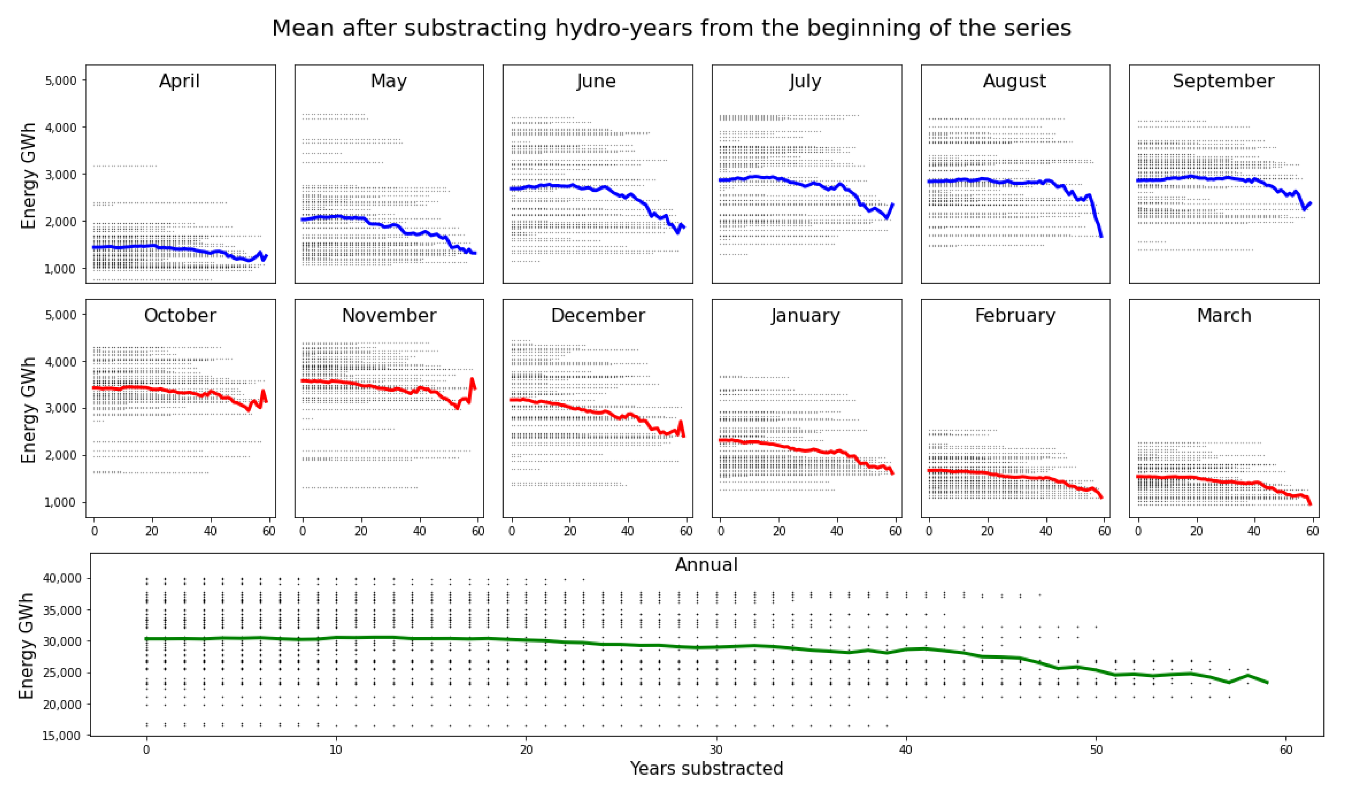
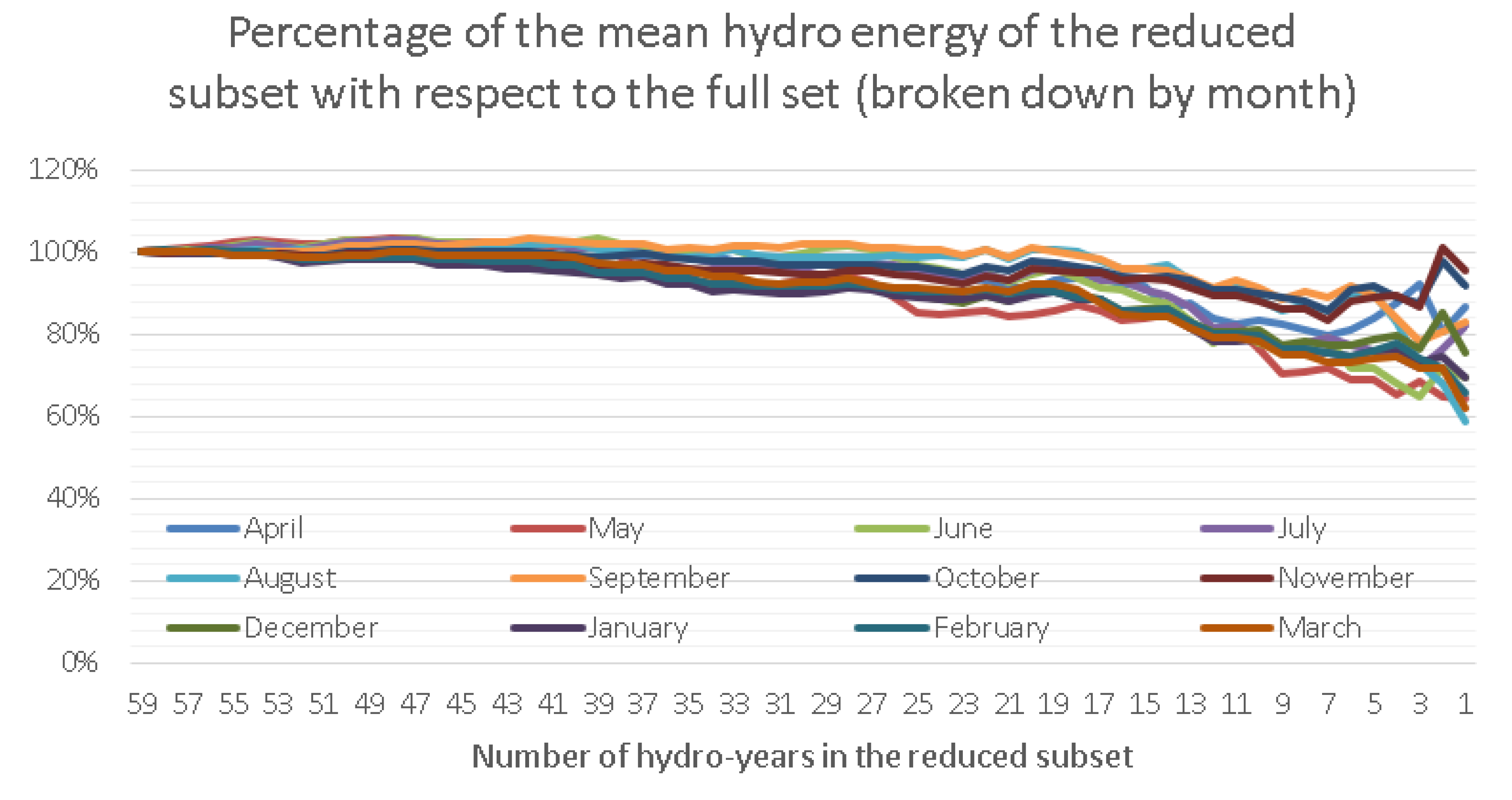
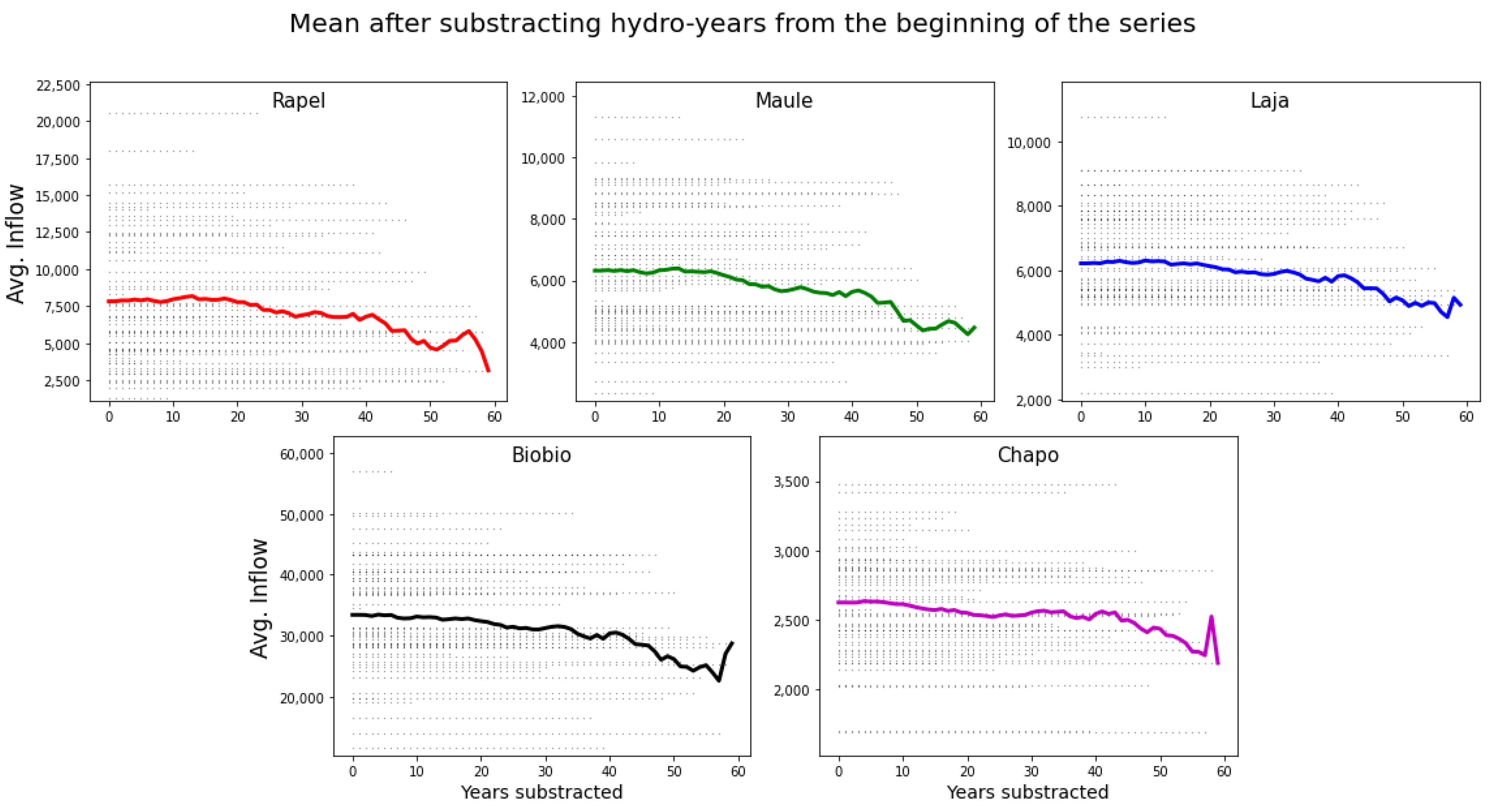
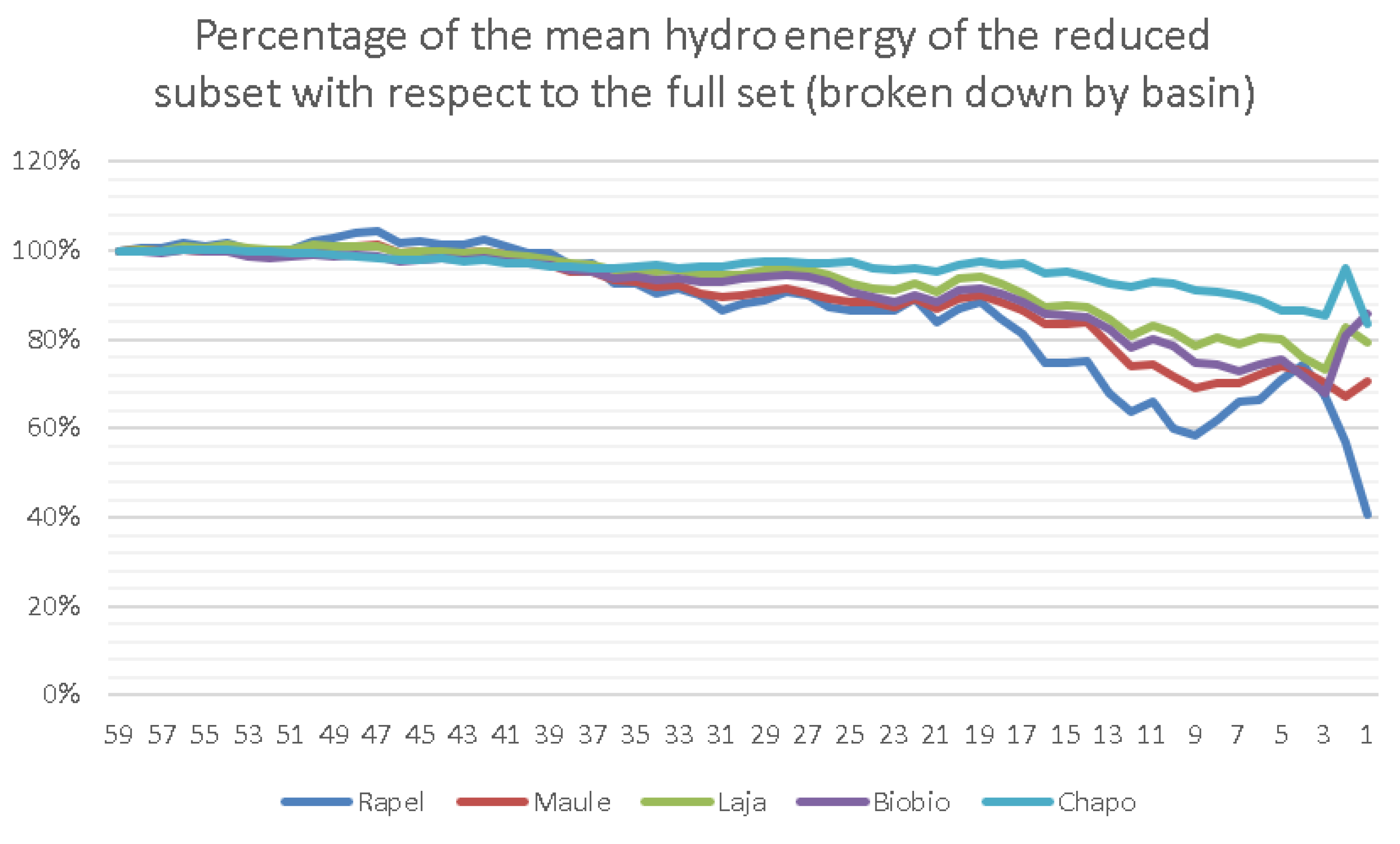
5.1. Analysis of the Mean Hydro-Inflows

Figure 6 shows the effect on the mean hydro-energy inflow of decreasing the number of hydro-years in the reduced subset, broken down by month. The reduced subset is produced by iteratively subtracting the first years of the time series, following Criterion 1. Starting with the complete time series, the number of years subtracted is represented in the horizontal axis. In the vertical axis, in small black dots, it is possible to see the energy associated with the cropped data. On the left, when there are no years subtracted, there are 59 black dots representing the 59 hydro-years of the original time series, for every month and for the whole year. As the number of years subtracted increases, the number of data points of the cropped time series reduces to one, consisting solely of the energy in GWh of the last hydro-year (2018–2019).
Figure 6 shows that as older hydro-years stop being considered in the subset (that is, more hydro-years are subtracted), the average energy of the subset tends to decrease. The impact of the MD on the right of the curves is more evident in the rainfall months than in the snowmelt season, as the reduction of hydro-energy inflow in the summer is somewhat dampened by the melting of the high-mountain snowpack. Figure 7 compares the mean hydro-energy of the reduced subset as a percentage of the mean of the full set. We observe that the last decade is approximately 80% drier than the average for the full set and that the percentage increases as the historically older (and wetter) years begin to be included in the set. In a subset of 16 hydro-years, the mean hydro-energy corresponds to approximately 90% of the mean for the full set. In a subset of 24 hydro-years, the mean hydro-energy corresponds to approximately 93% of the mean for the full set. A subset of this size is aligned with the simple guideline of 30 years provided by the WMO [53].
Figure 8 shows similar results to Figure 7 but broken down by month to illustrate the monthly trends in hydro-energy inflows. We observe that the period between May and July shows a more significant reduction in hydro-energy inflows than the spring and summer months, which are dominated by snowmelt.
Besides analyzing the intra-year behavior, it is essential to understand what is happening in different basins. Results disaggregated by basin are presented in Figure 9 and Figure 10. We observe that the impact of the MD is stronger in the northern basins (Rapel and Maule) but that there is also a longer trend of hydro-energy inflow reduction lasting at least 40 years in all the basins, confirming the impacts of climate change on Chilean hydrology.
Notice that using a reduced subset that is too small would risk losing some of the temporal and spatial trends and information contained in the data. For example, some recent off-trend inflows in Biobio and Chapo observed in the last few years could be lost if reducing the subset were excessively reduced. An analysis of the first, second and third quartiles (Q1, Q2 and Q3) in Figure 11 can help to visualize the presence of highly wet years in the 1960s in the Rapel and Maule basins, while the Laja, Biobio and Chapo basins remain stable for approximately the first two-thirds of the time series. Furthermore, the IQR seems to stabilize for subsets with over 20 hydro-years.
Based on the analysis of the hydro-trends, and according to Criterion 2 for selecting an alternative range of hydro-years, we suggest using only the last 20–30 years of data to represent the possible hydrology levels of the next years.

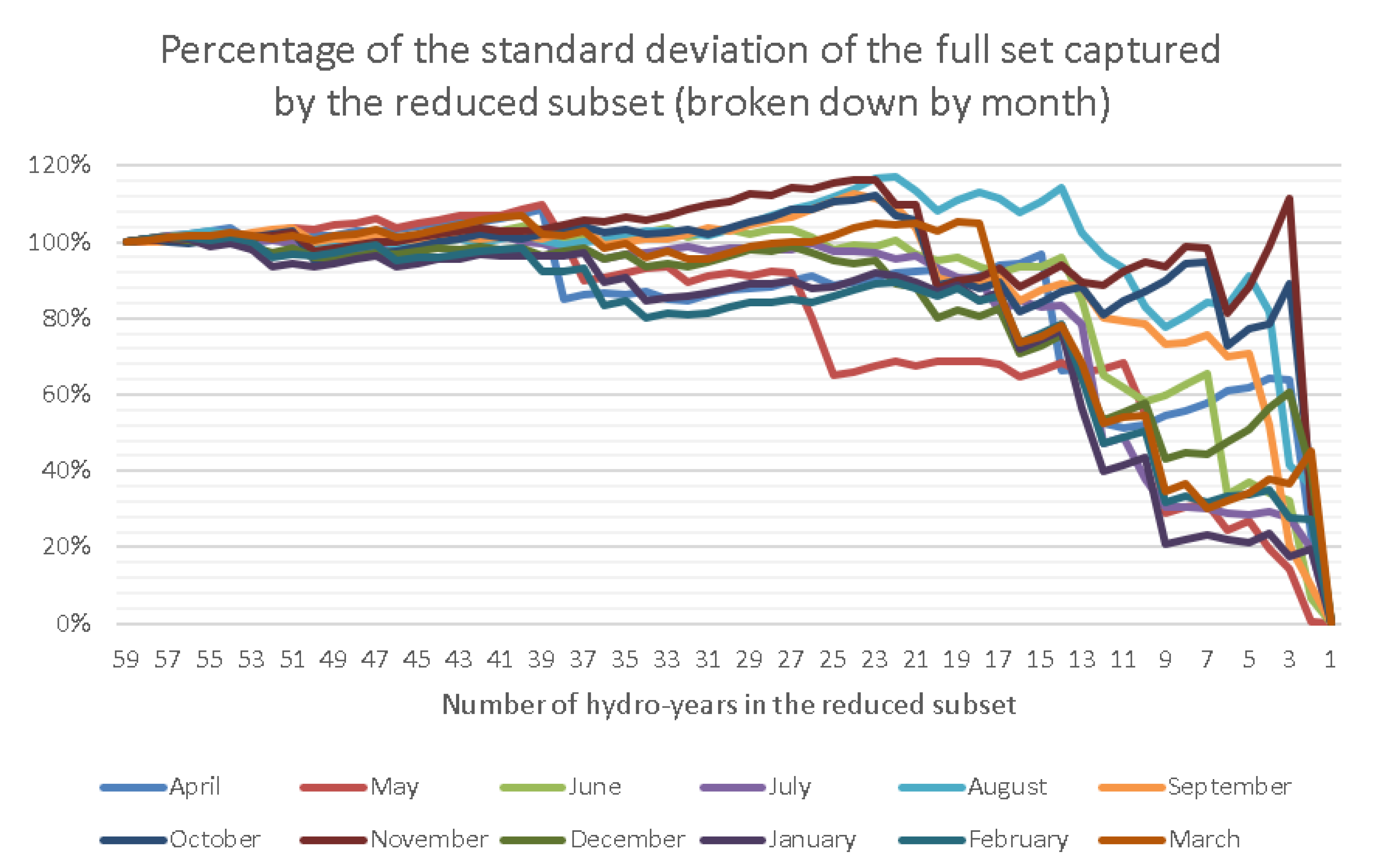
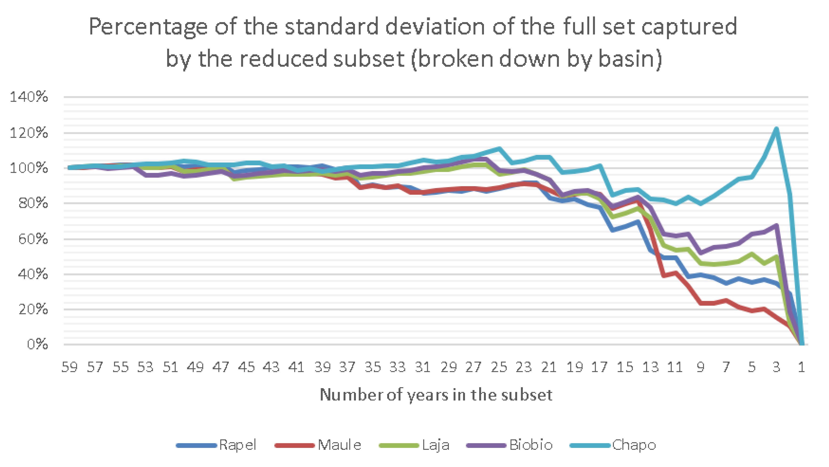
5.2. Analysis of the Variability of the Hydro Inflows

As established in [40] for the Nordic system, both the temporal and spatial distributions are important for representing hydro-uncertainty in SDDP-based scheduling models. Thus, while the analysis of the mean and quantiles of the reduced subsets are relevant to comply with Criterion 2 for selecting an alternative range of hydro-years, compliance with Criteria 3 to 5 requires the analysis of the variability of the reduced subset and for the intra-annual and spatial diversity of the data to be considered. Figure 12 and Figure 13 show the evolution of the standard deviation of the hydro-energy inflow in the reduced subset as older hydro-years are subtracted from the data. As the number of subtracted hydro-years increases, the number of data points tends to decrease. Naturally, the standard deviation reduces to zero when there is only one point remaining. The results in Figure 12 show that the first couple of months (April and May) experience sudden jumps in variability which are caused by unusual fall rains. Figure 13 shows that, with 24 hydro-years, the reduced subset can capture most of the inter-annual variability in the aggregated energy of the full set. Criterion 3 for the selection of an alternative range is reached with only 17 hydro-years.
Figure 14 shows that the standard deviation in most months stabilizes with over 20 years in the reduced subset. Furthermore, the goal set by Criterion 4 is reached with 20 years in the reduced subset for all months except May. As mentioned, this is caused by a few years with very unusual rains during the fall. However, although heavy fall precipitation used to occur once or twice per decade, it has not happened since 1993.
Figure 15 and Figure 16 show that the variability in the different basins tends to stabilize after 20 years, reaching the goal set by Criterion 5 with only 18 hydro-years in the reduced subset. The northern basins (Rapel and Maule) experienced the highest loss in variability, as most of their wet years were discarded.

6. Discussion of Results and Conclusions

The results in the previous section show that discarding the first three or four decades of historical hydro-data (i.e., using only data from the last two or four decades) would result in a reduced subset that is about 4% to 8% drier (in terms of total hydro-energy inflow) than when using the full set of 59 hydro-years. This would be aligned with the expectations for the reduction in precipitation and runoff reported in [44,46] for the next two decades, meeting the requirement established by Criterion 2. Regarding intra-annual and spatial variability, criteria 3, 4 and 5 for the selection of an alternative range of hydro-years are reached with 17, 20 and 18 hydro-years, respectively. Thus, with over 20 hydro-years in the reduced subset, we can adequately represent most of the intra-annual and spatial diversity of the data.
However, using only 20 years of data would miss the dry conditions observed in some hydro-years of the second half of the 1990s (1998–1999 and 1996–1997 were the driest and third-driest years on record). Furthermore, the standard deviation and IQR for the total hydro-energy inflow stabilizes after 24 years, as do the standard deviations for almost all months (except for May) and for most basins analyzed. Based on the discussion above and the criteria established in Section 4.2, we suggest the following two-step procedure to build an alternative hydrological dataset to include the impacts of hydro-uncertainty on Chilean’s electricity market simulations:
Step 1. Obtaining a reduced subset by discarding the older 35 hydro-years of hydrological data.
We propose to discontinue the use of the first 35 hydro-years of the series as they represent a different state of the climate system that does not correctly capture the impacts of ACF on Chilean hydrology. Instead, we suggest that only the last 24 hydro-years on record should be used to represent future hydro-uncertainty; that is, from hydro-year 1995–1996 to 2018–2019 (both inclusive). In other words, we propose to replace the use of the full set of 59 hydro-years by a reduced subset with the last 24 hydro-years. Of course, if data for hydro-year 2019–2020 or later become available, we would recommend including these data in the dataset as well. In our opinion and based on our predefined criteria, the loss of intra-annual and spatial variability caused by the shedding of 35 years of data remains within acceptable levels. Moreover, the lost variability is well below the levels of uncertainty in the energy market caused by other aspects, such as technological change or fuel prices. The resulting 24-hydro-year range would be approximately 7% drier on average than the full set of data, thereby already representing some of the anticipated effects of climate change on Chilean hydrology. However, if used by itself, this alternative range would not consider extreme scenarios whereby the MD currently being experienced in Chile could continue for an even more extended period; that is, there would not be any droughts longer than nine years in any of the 20-year-long sequences generated by the hydrothermal economic dispatch model. Thus, we also propose to additionally modify the dataset to consider more extreme drought scenarios in at least some of the simulations.
Step 2. Generate an extended subset by repeating the sequence of the last nine hydro-years at the end of the reduced subset defined in step 1.
This step considers repeating the sequence of the nine last hydro-years (2010–2011 to 2018–2019) at the end of the reduced 24 hydro-year sequence (1995–1996 to 2018–2019). This extended subset of 33 hydro-years would be approximately 10% drier (on average) than the full dataset and would also be aligned with [44,46] and the 30-year WMO guidelines [53]. Furthermore, this extended subset can be readily implemented in the model used by CNE in the same way that they include synthetic years. Considering a 20-year simulation horizon, some of the simulations will consider a drought lasting longer than nine years, thereby anticipating some of the most extreme impacts that climate change may have on Chilean hydrology.
Table 1 shows the main statistics of the reduced 24 hydro-year subset at the end of step 1 and the extended 33 hydro-year subset at the end of step 2. We observe that the extended subset is drier on average than the reduced subset (and both are drier than the full set). While the left-hand side and center of the distribution (quartiles Q1 and Q2) are very similar between the reduced and extended subsets (that is, dry and medium hydro-years), Q3 is significantly smaller. Thus, after step 2, the dataset implies a much lower probability of having wet years, which is well-aligned with the discussion in previous sections.
In summary, the alternative range of hydrological data proposed in this work captures some of the anticipated effects of climate change on hydro-uncertainty reported in the literature, while preserving most of the intra-annual and spatial diversity of the data.
Our analysis corroborates the need toaddress climate change in hydrology for electricity market modeling. For example, by post-processing CNE’s results published in [41], we observe that the alternative hydrological representation proposed in this study would yield average electricity prices between 4 and 5 USD/MWh higher than by using the full set of 59 hydro-years, depending on the location.
It is relevant to present a minor caveat here: two decades ago, most of the installed generation capacity in the SEN was hydroelectric. However, in the last two decades, the relative importance of hydro-generation has been consistently decreasing, as Figure 17 shows. Furthermore, only a small amount of new hydro-generation is expected to be built in the next decade. As a result, the impact that hydro-uncertainty may have on electricity prices in the SEN, while still significant, is continuously decreasing. Interestingly, despite the MD that has occurred in the present decade, spot electricity prices in the 2000s were higher than in the 2010s. Thus, besides hydrological conditions, electricity prices can also be driven by other factors such as fuel availability or the rise of emergent technologies. Although outside the scope of this report, there are other drivers that may be of more concern when assessing the risk of new electric generation projects, such as technological, societal or regulatory uncertainty.
Finally, it is also relevant to stress the difficulty in anticipating the complex dynamics of the climate system. The Earth’s climate is a complex system that involves interactions between the atmosphere, hydrosphere, cryosphere, lithosphere and biosphere [53]. Results from climate models are highly uncertain, as a result of a limited theoretical understanding of some processes and limited computing power. Despite the limitations of climate models, and given the evidence of drying in Central Chile, it is not adequate to continue considering hydrological data from six decades ago as equally likely to happen in the future. Thus, given the consensus amongst climate scientists regarding anthropogenic climate change, including its potential effects into risk assessment models should be standard practice. In this sense, our proposal for modeling future hydroelectric energy production in Chile offers a quick alternative representation of hydro-uncertainty that can better represent future market outcomes.

Author Contributions

Supervision, conceptualization and methodology, E.G.; investigation, E.G. and Y.M.; data analysis, E.G. and T.O.; writing—original draft preparation, E.G., Y.M., and T.O.; writing—review and editing, E.G. All authors have read and agreed to the published version of the manuscript.

Funding

This research was funded by Agencia Nacional de Investigación y Desarrollo (ANID) through grant number FB0008 (Advanced Center for Electrical and Electronic Engineering, AC3E). Additional funding was provided by Mainstream Renewable Power (MRP).

Institutional Review Board Statement

Not applicable.

Informed Consent Statement

Not applicable.

Data Availability Statement

Publicly available datasets were analyzed in this study. This data can be found here: https://www.cne.cl/en/tarificacion/electrica/precio-nudo-corto-plazo.

Acknowledgments

The authors would like to thank Brian Killen for proofreading an early draft of this work.

Conflicts of Interest

The analysis in this article is based on a technical report originally requested and funded by MRP. The funders had no role in the collection, analyses, or interpretation of data or in the conclusions of this article.

Abbreviations

The following abbreviations are used in this manuscript:
ACFAnthropogenic Climate Forcing
CENIndependent System Coordinator (Coordinador Eléctrico Nacional
CEPALUnited Nations Economic Commission for Latin America and the Caribbean (Comisión Económica para América Latina y el Caribe)
CNENational Energy Commission (Comisión Nacional de Energía)
ENSOEl Niño-Southern Oscillation
GCMGeneral Circulation Model
GHGGreenhouse gas emissions
GWhGigawatt-hour
IPCCThe Intergovernmental Panel on Climate Change
MDMega-drought
PDOPacific Decadal Oscillation
SAMSouthern Annular Mode
SENChilean interconnected system (Sistema Eléctrico Nacional)
SDDPStochastic Dual Dynamic Programming
WMOWorld Meteorological Organization

References

  1. IPCC. Climate change 2014: Synthesis report. In Contribution of Working Groups I, II and III to the Fifth Assessment Report of the Intergovernmental Panel on Climate Change; Pachauri, R., Meyer, L., Eds.; IPCC: Geneva, Switzerland, 2014. [Google Scholar]
  2. Seneviratne, S.; Nicholls, N.; Easterling, D.; Goodess, C.; Kanae, S.; Kossin, J.; Luo, Y.; Marengo, J.; McInnes, K.; Rahimi, M.; et al. Changes in climate extremes and their impacts on the natural physical environment. In Managing the Risks of Extreme Events and Disasters to Advance Climate Change Adaptation. A Special Report of Working Groups I and II of the Intergovernmental Panel on Climate Change (IPCC); Field, C., Barros, V., Stocker, T., Qin, D., Dokken, D., Ebi, K., Mastrandrea, M., Mach, K., Plattner, G.K., Allen, S., et al., Eds.; Cambridge University Press: Cambridge, UK; New York, NY, USA, 2012; Chapter 3; pp. 109–230. [Google Scholar]
  3. Trenberth, K.E. Changes in precipitation with climate change. Clim. Res. 2011, 47, 123–138. [Google Scholar] [CrossRef] [Green Version]
  4. Sun, Y.; Solomon, S.; Dai, A.; Portmann, R.W. How often will it rain? J. Clim. 2007, 20, 4801–4818. [Google Scholar] [CrossRef]
  5. Dai, A.; Zhao, T.; Chen, J. Climate change and drought: A precipitation and evaporation perspective. Curr. Clim. Chang. Rep. 2018, 4, 301–312. [Google Scholar] [CrossRef]
  6. Dai, A.; Rasmussen, R.M.; Liu, C.; Ikeda, K.; Prein, A.F. A new mechanism for warm-season precipitation response to global warming based on convection-permitting simulations. Clim. Dyn. 2020, 55, 343–368. [Google Scholar] [CrossRef]
  7. Forrest, K.; Tarroja, B.; Chiang, F.; AghaKouchak, A.; Samuelsen, S. Assessing climate change impacts on California hydropower generation and ancillary services provision. Clim. Chang. 2018, 151, 395–412. [Google Scholar] [CrossRef]
  8. Ehsani, N.; Vörösmarty, C.J.; Fekete, B.M.; Stakhiv, E.Z. Impact of a Warming Climate on Hydropower in the Northeast United States: The Untapped Potential of Non-Powered Dams. Preprints 2017, 2017110116. [Google Scholar] [CrossRef]
  9. Shevnina, E.; Pilli-Sihvola, K.; Haavisto, R.; Vihma, T.; Silaev, A. Climate change will increase potential hydropower production in six Arctic Council member countries based on probabilistic hydrological projections. Hydrol. Earth Syst. Sci. 2018. [Google Scholar] [CrossRef] [Green Version]
  10. Uamusse, M.M.; Aljaradin, M.; Nilsson, E.; Persson, K.M. Climate change observations into hydropower in Mozambique. Energy Procedia 2017, 138, 592–597. [Google Scholar] [CrossRef]
  11. Machina, M.B.; Sharma, S. Assessment of climate change impact on hydropower generation: A case study of Nigeria. Int. J. Eng. Technol. Sci. Res. 2017, 4, 753–762. [Google Scholar]
  12. Boadi, S.A.; Owusu, K. Impact of climate change and variability on hydropower in Ghana. Afr. Geogr. Rev. 2019, 38, 19–31. [Google Scholar] [CrossRef]
  13. Zhang, Y.; Gu, A.; Lu, H.; Wang, W. Hydropower generation vulnerability in the Yangtze River in China under climate change scenarios: Analysis based on the WEAP model. Sustainability 2017, 9, 2085. [Google Scholar] [CrossRef] [Green Version]
  14. Wang, H.; Xiao, W.; Wang, Y.; Zhao, Y.; Lu, F.; Yang, M.; Hou, B.; Yang, H. Assessment of the impact of climate change on hydropower potential in the Nanliujiang river basin of China. Energy 2019, 167, 950–959. [Google Scholar] [CrossRef]
  15. Liu, X.; Tang, Q.; Voisin, N.; Cui, H. Projected impacts of climate change on hydropower potential in China. Hydrol. Earth Syst. Sci. 2016, 20, 3343–3359. [Google Scholar] [CrossRef] [Green Version]
  16. Fan, J.L.; Hu, J.W.; Zhang, X.; Kong, L.S.; Li, F.; Mi, Z. Impacts of climate change on hydropower generation in China. Math. Comput. Simul. 2020, 167, 4–18. [Google Scholar] [CrossRef]
  17. Khaniya, B.; Priyantha, H.G.; Baduge, N.; Azamathulla, H.M.; Rathnayake, U. Impact of climate variability on hydropower generation: A case study from Sri Lanka. ISH J. Hydraul. Eng. 2020, 26, 301–309. [Google Scholar] [CrossRef]
  18. Shrestha, A.; Shrestha, S.; Tingsanchali, T.; Budhathoki, A.; Ninsawat, S. Adapting hydropower production to climate change: A case study of Kulekhani Hydropower Project in Nepal. J. Clean. Prod. 2020, 279, 123483. [Google Scholar] [CrossRef]
  19. Ali, S.A.; Aadhar, S.; Shah, H.L.; Mishra, V. Projected increase in hydropower production in India under climate change. Sci. Rep. 2018, 8, 1–12. [Google Scholar] [CrossRef] [Green Version]
  20. Caruso, B.; King, R.; Newton, S.; Zammit, C. Simulation of climate change effects on hydropower operations in mountain headwater lakes, New Zealand. River Res. Appl. 2017, 33, 147–161. [Google Scholar] [CrossRef]
  21. Teotónio, C.; Fortes, P.; Roebeling, P.; Rodriguez, M.; Robaina-Alves, M. Assessing the impacts of climate change on hydropower generation and the power sector in Portugal: A partial equilibrium approach. Renew. Sustain. Energy Rev. 2017, 74, 788–799. [Google Scholar] [CrossRef]
  22. Majone, B.; Villa, F.; Deidda, R.; Bellin, A. Impact of climate change and water use policies on hydropower potential in the south-eastern Alpine region. Sci. Total Environ. 2016, 543, 965–980. [Google Scholar] [CrossRef]
  23. Bombelli, G.M.; Soncini, A.; Bianchi, A.; Bocchiola, D. Potentially modified hydropower production under climate change in the Italian Alps. Hydrol. Process. 2019, 33, 2355–2372. [Google Scholar] [CrossRef]
  24. Savelsberg, J.; Schillinger, M.; Schlecht, I.; Weigt, H. The impact of climate change on Swiss hydropower. Sustainability 2018, 10, 2541. [Google Scholar] [CrossRef] [Green Version]
  25. Ritesh Patro, E.; Gaudard, L.; De Michele, C. Hydropower revenues under the threat of climate change: Case studies from Europe. Geophys. Res. Abstr. 2019, 21, EGU2019-320-1. [Google Scholar]
  26. de Queiroz, A.R.; Lima, L.M.M.; Lima, J.W.M.; da Silva, B.C.; Scianni, L.A. Climate change impacts in the energy supply of the Brazilian hydro-dominant power system. Renew. Energy 2016, 99, 379–389. [Google Scholar] [CrossRef]
  27. de Oliveira, V.A.; de Mello, C.R.; Viola, M.R.; Srinivasan, R. Assessment of climate change impacts on streamflow and hydropower potential in the headwater region of the Grande river basin, Southeastern Brazil. Int. J. Climatol. 2017, 37, 5005–5023. [Google Scholar] [CrossRef]
  28. de Souza Dias, V.; Pereira da Luz, M.; Medero, G.M.; Tarley Ferreira Nascimento, D. An overview of hydropower reservoirs in Brazil: Current situation, future perspectives and impacts of climate change. Water 2018, 10, 592. [Google Scholar] [CrossRef] [Green Version]
  29. de Queiroz, A.R.; Faria, V.A.; Lima, L.M.; Lima, J.W. Hydropower revenues under the threat of climate change in Brazil. Renew. Energy 2019, 133, 873–882. [Google Scholar] [CrossRef]
  30. Hasan, M.M.; Wyseure, G. Impact of climate change on hydropower generation in Rio Jubones Basin, Ecuador. Water Sci. Eng. 2018, 11, 157–166. [Google Scholar] [CrossRef]
  31. Arriagada, P.; Dieppois, B.; Sidibe, M.; Link, O. Impacts of climate change and climate variability on hydropower potential in data-scarce regions subjected to multi-decadal variability. Energies 2019, 12, 2747. [Google Scholar] [CrossRef] [Green Version]
  32. Oyerinde, G.T.; Wisser, D.; Hountondji, F.C.; Odofin, A.J.; Lawin, A.E.; Afouda, A.; Diekkrüger, B. Quantifying uncertainties in modeling climate change impacts on hydropower production. Climate 2016, 4, 34. [Google Scholar] [CrossRef] [Green Version]
  33. Wen, X.; Liu, Z.; Lei, X.; Lin, R.; Fang, G.; Tan, Q.; Wang, C.; Tian, Y.; Quan, J. Future changes in Yuan River ecohydrology: Individual and cumulative impacts of climates change and cascade hydropower development on runoff and aquatic habitat quality. Sci. Total Environ. 2018, 633, 1403–1417. [Google Scholar] [CrossRef] [PubMed]
  34. Guerra, O.J.; Tejada, D.A.; Reklaitis, G.V. Climate change impacts and adaptation strategies for a hydro-dominated power system via stochastic optimization. Appl. Energy 2019, 233, 584–598. [Google Scholar] [CrossRef]
  35. Feng, Y.; Zhou, J.; Mo, L.; Yuan, Z.; Zhang, P.; Wu, J.; Wang, C.; Wang, Y. Long-term hydropower generation of cascade reservoirs under future climate changes in Jinsha River in Southwest China. Water 2018, 10, 235. [Google Scholar] [CrossRef] [Green Version]
  36. François, B.; Hingray, B.; Borga, M.; Zoccatelli, D.; Brown, C.; Creutin, J.D. Impact of climate change on combined solar and run-of-river power in northern Italy. Energies 2018, 11, 290. [Google Scholar] [CrossRef] [Green Version]
  37. Pilesjo, P.; Al-Juboori, S.S. Modelling the effects of climate change on hydroelectric power in Dokan, Iraq. Int. J. Energy Power Eng. 2016, 5, 7. [Google Scholar] [CrossRef] [Green Version]
  38. Miao, C.; Su, L.; Sun, Q.; Duan, Q. A nonstationary bias-correction technique to remove bias in GCM simulations. J. Geophys. Res. Atmos. 2016, 121, 5718–5735. [Google Scholar] [CrossRef]
  39. Pereira, M.V.; Pinto, L.M. Multi-stage stochastic optimization applied to energy planning. Math. Program. 1991, 52, 359–375. [Google Scholar] [CrossRef]
  40. Gjerden, K.S.; Helseth, A.; Mo, B.; Warland, G. Hydrothermal scheduling in Norway using stochastic dual dynamic programming; a large-scale case study. In Proceedings of the 2015 IEEE Eindhoven PowerTech, Eindhoven, The Netherlands, 29 June–2 July 2015; pp. 1–6. [Google Scholar] [CrossRef]
  41. CNE. Fijación de precios de nudo de corto plazo: Informe Técnico Definitivo; Technical Report; Comisión Nacional de Energía: Santiago, Chile, 2020. [Google Scholar]
  42. Dictuc. Análisis de la estadística hidrológica empleada para la estimación del precio de nudo del SIC; Technical Report; Dictuc: Santiago, Chile, 1999. [Google Scholar]
  43. Boisier, J.P.; Rondanelli, R.; Garreaud, R.D.; Muñoz, F. Anthropogenic and natural contributions to the Southeast Pacific precipitation decline and recent megadrought in central Chile. Geophys. Res. Lett. 2016, 43, 413–421. [Google Scholar] [CrossRef] [Green Version]
  44. Bozkurt, D.; Rojas, M.; Boisier, J.P.; Valdivieso, J. Climate change impacts on hydroclimatic regimes and extremes over Andean basins in central Chile. Hydrol. Earth Syst. Sci. Discuss 2017, 2017, 1–29. [Google Scholar]
  45. Bozkurt, D.; Rojas, M.; Boisier, J.P.; Valdivieso, J. Projected hydroclimate changes over Andean basins in central Chile from downscaled CMIP5 models under the low and high emission scenarios. Clim. Chang. 2018, 150, 131–147. [Google Scholar] [CrossRef]
  46. McPhee, J. Análisis de la vulnerabilidad del sector hidroeléctrico frente a escenarios futuros de cambio climático en Chile; Technical Report; UN-CEPAL: Santiago, Chile, 2012. [Google Scholar]
  47. Garreaud, R.D.; Boisier, J.P.; Rondanelli, R.; Montecinos, A.; Sepúlveda, H.H.; Veloso-Aguila, D. The central Chile mega drought (2010–2018): A climate dynamics perspective. Int. J. Climatol. 2020, 40, 421–439. [Google Scholar] [CrossRef]
  48. CR2. La megasequía 2010–2015: Una lección para el futuro; Technical Report; Centro de Ciencia del Clima y la Resiliencia (CR)2: Santiago, Chile, 2015. [Google Scholar]
  49. DGA. Balance Hídrico de Chile; Technical Report; Dirección General de Aguas: Santiago, Chile, 2019. [Google Scholar]
  50. Garreaud, R.D.; Alvarez-Garreton, C.; Barichivich, J.; Boisier, J.P.; Christie, D.; Galleguillos, M.; LeQuesne, C.; McPhee, J.; Zambrano-Bigiarini, M. The 2010–2015 megadrought in central Chile: Impacts on regional hydroclimate and vegetation. Hydrol. Earth Syst. Sci. 2017, 21, 6307–6327. [Google Scholar] [CrossRef] [Green Version]
  51. Morales, Y.; Olivares, M.; Vargas, X. Improving the flow representation in a stochastic programming model for hydropower operations in Chile. In Proceedings of the American Geophysical Union, Fall Meeting, San Francisco, CA, USA, 14–18 December 2015. [Google Scholar]
  52. Aravena, I.; Gil, E. Hydrological scenario reduction for stochastic optimization in hydrothermal power systems. Appl. Stoch. Models Bus. Ind. 2015, 31, 231–240. [Google Scholar] [CrossRef]
  53. IPCC. Annex III. Glossary: IPCC—Intergovernmental Panel on Climate Change; Planton, S., Ed.; IPCC Fifth Assessment Report; IPCC: Geneva, Switzerland, 2013; p. 1450.
Figure 1. The graph above shows the decreasing trend of the hydro-energy inflows from the six decades on record. The lower graph shows the percentiles of each hydro-year, with the marks indicating the rank of each year (from driest to wettest).
Energies 14 00241 g001
Figure 2. Classification of hydro-years into “wet”, “normal” and “dry” clusters (blue, yellow and red, respectively) using the k-means algorithm regarding the hydro-energy inflows. Six of the 10 dry years belong to the decade starting in 2010, which illustrates the effect that the mega-drought has on the available hydro-energy in the SEN.
Energies 14 00241 g002
Figure 3. Yearly hydro-energy inflow (GWh). The lines in the grey band corresponds to quartiles Q1, Q2 and Q3.
Energies 14 00241 g003
Figure 4. Yearly hydro-energy inflow (GWh) sorted by decade. The lines in the grey bands correspond to quartiles Q1, Q2 and Q3 for the decade.
Energies 14 00241 g004
Figure 5. Average hydro-energy inflow per month, sorted by decade. Every month in the last decade has been drier than in any other decade.
Energies 14 00241 g005
Figure 6. Mean hydro-energy inflow of the reduced subset of hydro-years against subtracted years broken down by month. The scale of the horizontal and vertical axes is the same for every plot, with the exception of the annual plot. The lines represent the mean hydro-energy inflow of each reduced subset. Blue and red represent the rainfall and snowmelt season, respectively.
Energies 14 00241 g006
Figure 7. Percentage of the mean hydro-energy of the reduced subset with respect to the full set (total for hydro-year).
Energies 14 00241 g007
Figure 8. Percentage of the mean hydro-energy of the reduced subset with respect to the full set (broken down by month).
Energies 14 00241 g008
Figure 9. Mean hydro-energy inflow of the reduced subset of hydro-years against subtracted years broken down by basin. The lines represent the mean hydro-inflow of each reduced subset. The plots are ordered from the top left to right corner according to their locations from north to south.
Energies 14 00241 g009
Figure 10. Percentage of the mean hydro-energy of the reduced subset with respect to the full set (broken down by basin).
Energies 14 00241 g010
Figure 11. Quartiles of the hydro-energy inflow of the reduced subset of hydro-years against subtracted years broken down by basin. The lines represent quartiles Q1, Q2 and Q3 of each reduced subset. When there is only one data point, all the quartiles coincide with the remaining data point energy value. The plots are ordered from the top-left to the bottom-right corner in accordance with their locations from north to south. Each plot has a different vertical scale, as the levels of water availability are highly different.
Energies 14 00241 g011
Figure 12. Standard deviation of the hydro-energy inflow of the reduced subset of hydro-years against subtracted years broken down by month. The scale of the horizontal and vertical axes is the same for every plot, with the exception of the annual plot. The lines represent the standard deviation of the hydro-energy inflow of each reduced subset. For better visualization, a double vertical axis is employed, where the standard deviation scale is specified on the right and remains the same for every month. Blue and red represent the rainfall and snowmelt season, respectively.
Energies 14 00241 g012
Figure 13. Percentage of the standard deviation of the full set captured by the reduced subset (total for hydro-year).
Energies 14 00241 g013
Figure 14. Percentage of the standard deviation of the full set captured by the reduced subset (broken down by month).
Energies 14 00241 g014
Figure 15. Standard deviation of the hydro-energy inflow of the reduced subset of hydro-years against subtracted years broken down by basin. The lines represent the standard deviation of the hydro-inflow of each reduced subset. The plots are ordered from top left to right corners according to their locations from north to south.
Energies 14 00241 g015
Figure 16. Percentage of the standard deviation of the full set captured by the reduced subset (broken down by basin).
Energies 14 00241 g016
Figure 17. Actual and projected percentage of hydro and non-hydro installed capacity in the SEN.
Energies 14 00241 g017
Table 1. Main statistics of the reduced subset and the extended subset. IQR: inter-quartile range.
StatisticBusiness as UsualAfter Step 1After Step 2
(GWh)Full SetReduced SubsetExtended Subset
of Hydro-Yearswith 24 Hydro-Yearswith 33 Hydro-Years
Min16,52416,52416,524
Max39,90337,66937,669
Max–Min23,37921,14521,145
Average30,29528,29127,261
Std. dev.571759485436
Q126,56823,43823,347
Q2 (median)30,54126,82526,538
Q334,52133,57030,674
IQR795310,1327327
Publisher’s Note: MDPI stays neutral with regard to jurisdictional claims in published maps and institutional affiliations.

