Identification of Extreme Wind Events Using a Weather Type Classification

Abstract

The identification of extreme wind events and their driving forces are crucial to better integrating wind generation into the power system. Recent work related the occurrence of extreme wind events with some weather circulation patterns, enabling the identification of (i) wind power ramps and (ii) low-generation events as well as their intrinsic features, such as the intensity and time duration. Using Portugal as a case study, this work focuses on the application of a weather classification-type methodology to link the weather conditions with wind power generation, namely, the different types of extreme events. A long-term period is used to assess and characterize the changes in the occurrence of extreme weather events and corresponding intensity on wind power production. High variability is expected under cyclonic regimes, whereas low-generation events are most common in anticyclonic regimes. The results of the work provide significant insights regarding wind power production in Portugal, enabling an increase in its predictability.

1. Introduction

To mitigate climate change, the decarbonization of our society is mandatory and has been encouraged by policymakers. One of the main measures to accomplish the desired decarbonization is the transition from conventional fossil fuels to low levels or to zero-carbon renewable energy technologies, which, in combination with energy-saving measures such as higher energy efficiency, will contribute to mitigating the impacts of climate change [1]. In this sense, renewable energies such as solar photovoltaic (PV) and wind represent key elements in the energy supply, now and in the near future. As an example, according to the national energy and climate plans of European Union countries, 80% of the new installed capacity will be based on renewable energy systems, namely, wind technology (onshore and offshore), which may become the main source of energy in the coming decades [2]. In the Portuguese case, this technology will increase from the current 5.4 GW to 9.3 GW (9.0 GW onshore and 0.3 offshore) [2].

Despite the environmental benefits of renewable energy sources, their weather-dependent nature and the intrinsic time and spatial variability of primary resources, as well as their poor predictability, often hinders their integration into power systems, especially when integrated on a large scale. This behavior differs from conventional power plants (e.g., coal, natural gas, and hydroelectric power plants), which can be easily managed to counterbalance, each time, the electricity demand to keep the power system stable. Conversely, taking into account the emergence of nearly 100% renewable energy systems, the conventional/fossil power plants tend to disappear, and with them, their support of flexibility needs. On the other hand, in some regions such as in the Iberian Peninsula, the impact of climate change will definitely change the water cycle, which affects precipitation and, consequently, the availability of hydro generation, increasing dependency on wind and solar power generation. Therefore, a long-term comprehensive approach, including an economic analysis, is required to promote the large-scale integration of wind and solar PV into power systems for the attenuation/minimization of climate change [1,3].

To support this holistic approach, new concepts need to be properly adopted, such as electrical grid interconnection over large regions (to facilitate the import of renewable electricity from remote regions), demand response (changing or reducing electricity demand to match the binomial supply/demand), sector coupling, and the use of energy storage technologies (which enables energy from times of abundance to be used in times of shortfall) [4]. However, to support a desirable carbon-free power system, these solutions may be insufficient under certain conditions, e.g., if there is no renewable generation capable of balancing the energy demand. Therefore, understanding the meteorological driving forces of power generation variability and extreme events is crucial to better integrating renewable power sources into the power system by helping to prevent its failure and minimize the impact of such forces from a technical and economical point of view. “Extreme events” refers to the so-called wind power ramps, but also to some other relevant phenomena such as energy droughts and low-generation events [3,5].

An approach commonly used in meteorology to improve the knowledge of the underlying role of meteorological conditions in a specific phenomenon is the use of weather circulation pattern approaches. These approaches enable the complexity of meteorological variability to be reduced, enabling the most common patterns in the climate system to be identified. These patterns are commonly defined through meteorological patterns on a synoptic scale, such as mean sea level pressure or geopotential height fields, and can be grouped into meteorological classifications. Other approaches can be found in the literature [2,3,4,5,6]. In [6], the authors applied a Grosswetterlagen classification to assess the meteorological conditions that would lead to extreme conditions—extremely high energy shortfall and extremely low renewable energy production. Although this type of approach is essential to understanding the driving forces of a specific phenomenon, in the last few years, machine learning approaches have also been developed and applied to accurately predict the wind speed/power variability and the occurrence of extreme wind power events [7,8,9,10,11].

Currently, the literature regarding the link between Portuguese wind power variability and meteorological conditions is still limited. Nevertheless, the connection between large-scale atmospheric circulation patterns and monthly wind power resources with the wind power production in mainland Portugal was analyzed in [12] using three circulation patterns: the North Atlantic Oscillation (NAO), the East Atlantic Pattern (EA), and the Scandinavian Pattern (SCAND). The authors showed that wind power variability in mainland Portugal during winter is influenced by the NAO and EA patterns. Regarding extreme events, special attention has been given to the so-called wind power ramps. In [11], a sequence of weather regimes was connected to the occurrence of those events, whereas in [13] the authors applied two different algorithms to identify, in an early phase, the existence of wind power ramps.

Using Portugal as a case study, this work contributes to understanding and characterizing wind power variability based on a well-known Lamb-based weather classification-type methodology adapted for the region under analysis. The characterization will enable an increase in wind power generation predictability, especially during extreme wind power events, ensuring that the underlying role of weather conditions is dully perceived. In order to assess the intensity changes and the occurrence of extreme weather events in wind energy production, a long-term period was used.

2. Data and Methodology

2.1. Data

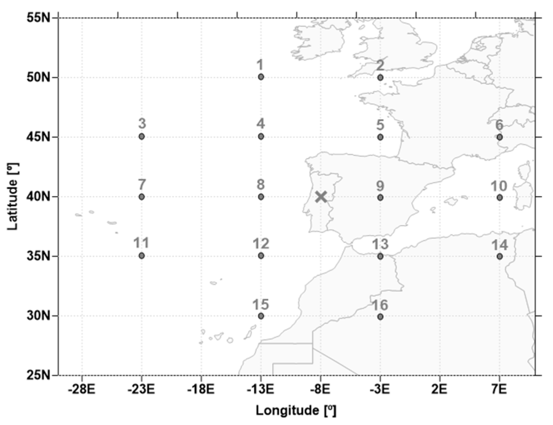
2.1.1. Meteorological Data—Atmospheric Reanalyses

The role and importance of atmospheric reanalyses for climate monitoring is now widely recognized, with the first generation comprising three datasets: the NCEP-R1 [14], the ERA-40 [15], and the JRA-25 [16]. Later, the NCEP-R1 was improved by fixing some errors and by updating the model parametrizations. As a result, a new product, NCEP-R2 [17], was released. This procedure also occurred for the remaining datasets. Nowadays, among reanalysis datasets the most widely used are the following: the NCEP-R2, the NCEP-CFSv2 [18], the ECMWF ERA-Interim [15], and the NASA MERRA-2 [16]. Recently, the ECMWF released the ERA5 reanalysis, replacing the former ERA-Interim products since this new product presents much higher temporal and spatial resolutions (1 h and nearly 31 km, respectively) compared to the aforementioned reanalyses. This product is being developed within the Copernicus Climate Change Service (C3S) and several authors have already highlighted the substantial improvement with respect to other similar products [19].

In this work, the ERA-5 reanalysis data were used and processed for the period from January 1950 to December 2019 (70 years of data) with hourly resolution.

2.1.2. Wind Power Data

In the latest years, there has been an effort from the scientific community to provide renewable generation data series (e.g., wind and solar PV), for long-term modelling and mitigation of the impact of the penetration of these energy sources in the electrical systems [20]. Typically, this information is derived from meteorological data sources such as reanalysis. Examples of these databases are (i) Renewables.ninja web tool [21] and (ii) the EMHires—European Meteorological derived HIgh resolution RES generation time series produced by the Joint Research Center [22]. In the first dataset, the authors establish a methodology based on a virtual wind power plant using NASA MERRA reanalysis with a bias correction. The EMHires dataset also uses the same reanalysis, although in this case, the authors use information on the locations of existing wind parks and the results are normalized, taking into account the annual statistics published by ENTSO-E.

The validation of these datasets has been carried out by several authors, showing that they are able to describe wind power production behavior in reasonable detail and present an annual average similar to the one reported by the transmission system operators [23,24]. However, for the specific case of Portugal, in [23] the authors showed some deviations between the observed and EMHires’ simulated wind power load duration curve, whereas in [24], the author identified difficulties of these datasets in properly describing the daily average production profile, a very important feature of wind power production. To overcome these limitations, [24] implemented a measure correlate predict (MCP) methodology using data from the ERA-5 database coupled with principal component analysis and artificial neural networks. The approach was calibrated using the national aggregated wind power data during 2019–2020. Figure 1 presents the daily average wind power capacity factor for different datasets and the observed profile.

Figure 1 clearly highlights that the MCP approach is the only one capable of following the observed daily profile, preserving one of the most relevant features of wind power generation in Portugal. These results are supported by the hourly correlation data for the different datasets (

Table 1. Correlation value for different publicly available datasets and the national aggregated wind power production—January 2014 to December 2015.

EMHires	Renewables.ninja	MCP
0.88	0.86	0.94

).

According to this table, the MCP also shows the best performance regarding the Pearson correlation. Thus, to obtain a long-term database, the MCP approach was used to estimate the wind power capacity factors from 1980 to 2018.

2.2. Methodology

2.2.1. Wind Power Variability and Extreme Events

The knowledge of the wind power variability and the occurrence of extreme events (such as wind power ramps) and low generation events contribute to the characterization of risk of operating power systems in moments of great variability or absence of suitable resources. Additionally, it allows for the mitigation of technical and economic consequences, e.g., through dynamic allocation of additional power reserves. For this reason and due to the high growth of wind penetration into power systems in recent years, the importance and relevance of characterizing these events has grown in the last few years.

However, a characterization and definition of these events is very difficult to obtain, since it varies from system to system, and it needs to be defined according to the technical characteristics of the electrical system in which it is inserted [5]. In this sense, unanimous definitions have not yet been established [13].

In the case of wind power ramps, the definition is related to the notion of an event that is sufficiently serious to merit special attention. This sensitive classification is related to the potential damages and costs associated with poor or inadequate management of the event that is considered too high (or sufficient) to be able to be distinguished from situations without a ramp [5]. Another definition, a little more specific, consists of a sudden and significant change in the wind power generation injected into the electric grid by a wind power plant or an aggregation of wind parks in a way that requires a more or less untimely readjustment of the power system. According to [25], whenever there is a variation in the energy produced with sufficient amplitude in a relatively short period of time, one is in the presence of a ramp. In this case, the authors considered that this variation needs to be at least 50% of the installed capacity for a period of time in the order of 4 h or less. To overcome the previous drawbacks, the following definition was used in this work:

$$\mathrm{Ramp}-\mathrm{up}: \underset{}{\max }\left(\mathrm{CapacityFactor}\left(t+∆t\right)-\mathrm{CapacityFactor}\left(t\right)\right)$$

(1)

$$\mathrm{Ramp}-\mathrm{down}: \underset{}{\min }\left(\mathrm{CapacityFactor}\left(t+∆t\right)-\mathrm{CapacityFactor}\left(t\right)\right)$$

(2)

In the previous equations, t represents the time and $∆t$ the time interval. Here, different values for $∆t$ were assumed and the type of ramp was calculated for the entire day under analysis to be later assigned to the respective weather regime. It is important to notice that this definition of ramp detection focuses only on the end and starting points of the interval. Eventual ramps that may occur during this interval are neglected.

Another relevant extreme event is the so-called low-generation event [26]. These events are characterized by a reduced availability of wind resources, and therefore, during these periods other technologies need to be explored to suppress the demand.

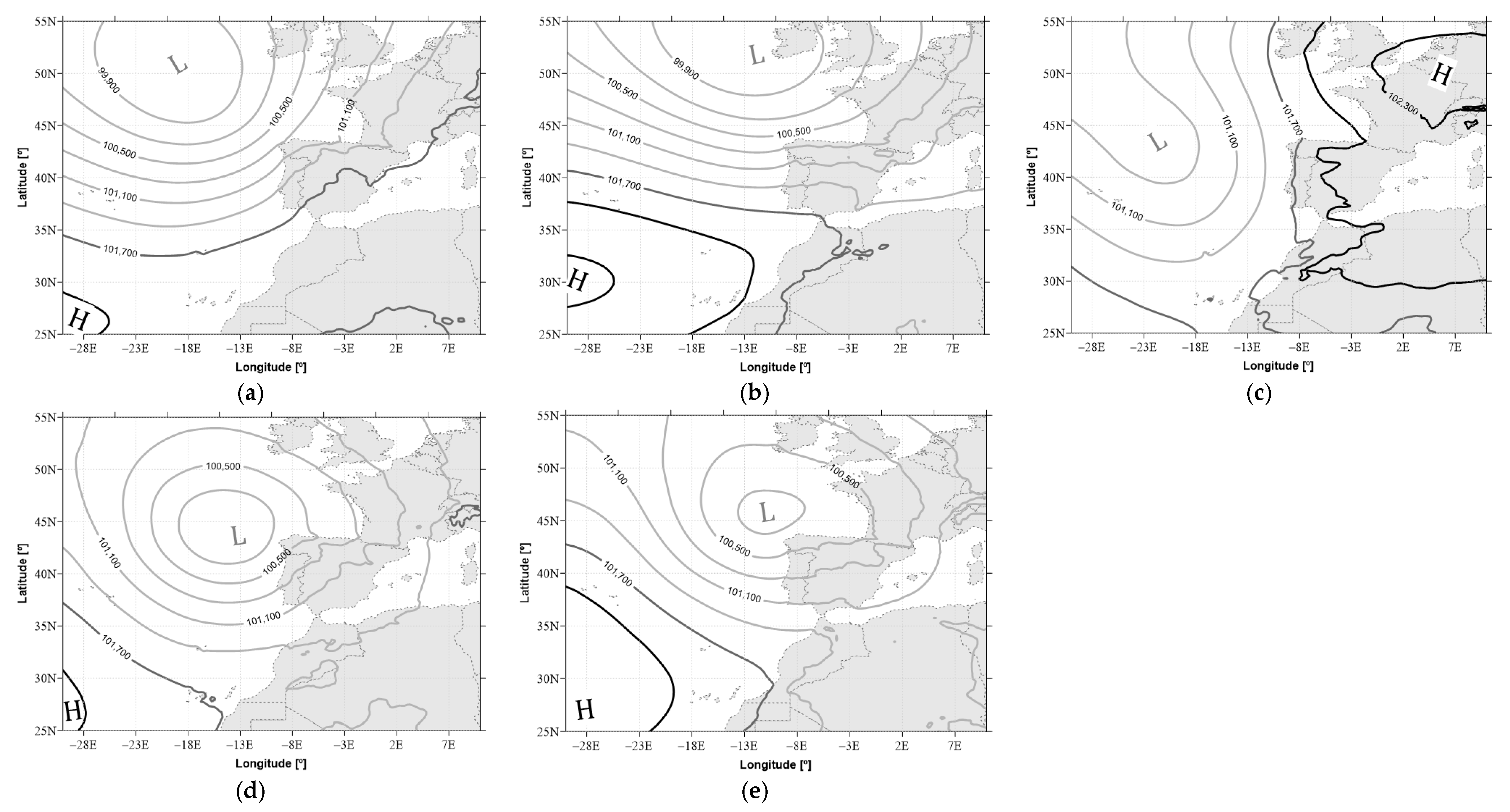
2.2.2. Weather Classification Approach

The weather circulation-type classification enables 26 distinct weather patterns to be identified using mean sea level surface pressure reanalysis data obtained from the project ERA5. Atmospheric circulation state classification into different types is a widely used technique to describe and analyze weather patterns and their impact on a predetermined parameter. Currently, it is possible to find several weather circulation classifications in the literature [27,28]. In [29], a validation of the classification was developed and the authors emphasized the quality of the most recent reanalysis databases in providing better estimates against old reanalysis databases. In [30], this classification was employed to estimate pan-European wind power generation coupled with a spatio-temporal clustering approach. The authors identified that training a model for different prevailing weather situations enables a small set of reference sites to be used without reducing the accuracy.

The main focus of this study is the use of an automatic version of the Lamb weather-type classification method (WT) initially proposed by [31] and already applied and tested by several authors, e.g., [32,33,34]. The main advantage of using a Lamb-based classification rather than other classification methodologies—commonly based on automated neural networks (ANN) or clustering techniques—is the capability of provide the full meteorological physical meaning of the results. The Lamb weather-type classification assumes that the wind circulation is almost geostrophic near the surface and uses the mean sea level pressure on a grid with 16 points around a central grid point for which the classification is performed [32] (Figure 2).

The weather circulation types are identified for each day for a central latitude point. The 16 grid points are equally spaced by 10° and 5° for latitudes and longitudes, respectively, around the central point. For the present study, the central point was chosen in the middle of mainland Portugal, where most wind parks are located, and where data referring to long-term wind capacity were available for the current study.

In this sense, the first step towards the weather classification is the computation of six circulation indexes (

Table 2. Classification indexes. Adapted from [32].

Circulation Indexes	Flow Features
SF	North–south direction
WF	West–east direction
FT	Flow magnitude
ZS	Low-pressure circulation
ZW	High-pressure circulation
ZT	Relative vorticity

), which are associated with (i) the wind flow direction, (ii) the circulation type—high- or low-pressure circulation, and (iii) the geostrophic vorticity and divergence at the surface. For each day, the six circulation indexes were calculated using Equations (1)–(10) [31] based on the mean sea level pressure (MSLP) over 16 grid points, allowing the classification of 26 different weather circulation types.

$$SF=Coe{f}_1\times \left[0.25\times \left(p_5+2p_9+p_{13}\right)-0.25\times \left(p_4+2\times p_8+p_{12}\right)\right]$$

(3)

$$WF=\left[0.5\times \left(p_{12}+p_{13}\right)-0.5\times \left(p_4+p_5\right)\right]$$

(4)

$$FT=\sqrt{S{F}^2+W{F}^2}$$

(5)

$$ZS=Coe{f}_2\times \left[0.25\times \left(p_6+2p_{10}+p_{14}\right)-0.25\times \left(p_5+2p_9+p_{13}\right)-0.25\times \left(p_4+2p_8+p_{12}\right)+0.25\times \left(p_3+2p_7+p_{11}\right)\right]$$

(6)

$$\begin{array}{r}ZW=Coe{f}_3\times \left[0.5\times \left(p_{15}+p_{16}\right)-0.5\times \left(p_8+p_9\right)\right]\\ -Coe{f}_4\times \left[0.5\times \left(p_8+p_9\right)-0.5\times \left(p_1+p_2\right)\right]\end{array}$$

(7)

$$ZT=ZS+ZW$$

(8)

$$Coe{f}_1=\frac{1}{\cos \left(\psi \right)}$$

(9)

$$Coe{f}_2=\frac{1}{2\times \cos {\left(\psi \right)}^2}$$

(10)

$$Coe{f}_3=\frac{\sin \left(\psi \right)}{\sin \left(\psi -5°\right)}$$

(11)

$$Coe{f}_4=\frac{\sin \left(\psi \right)}{\sin \left(\psi +5°\right)}$$

(12)

where $\psi$ denotes the central latitude point of the domain (“x” in Figure 2), 40° in this case. The daily classification was established in accordance with the following rules:

-

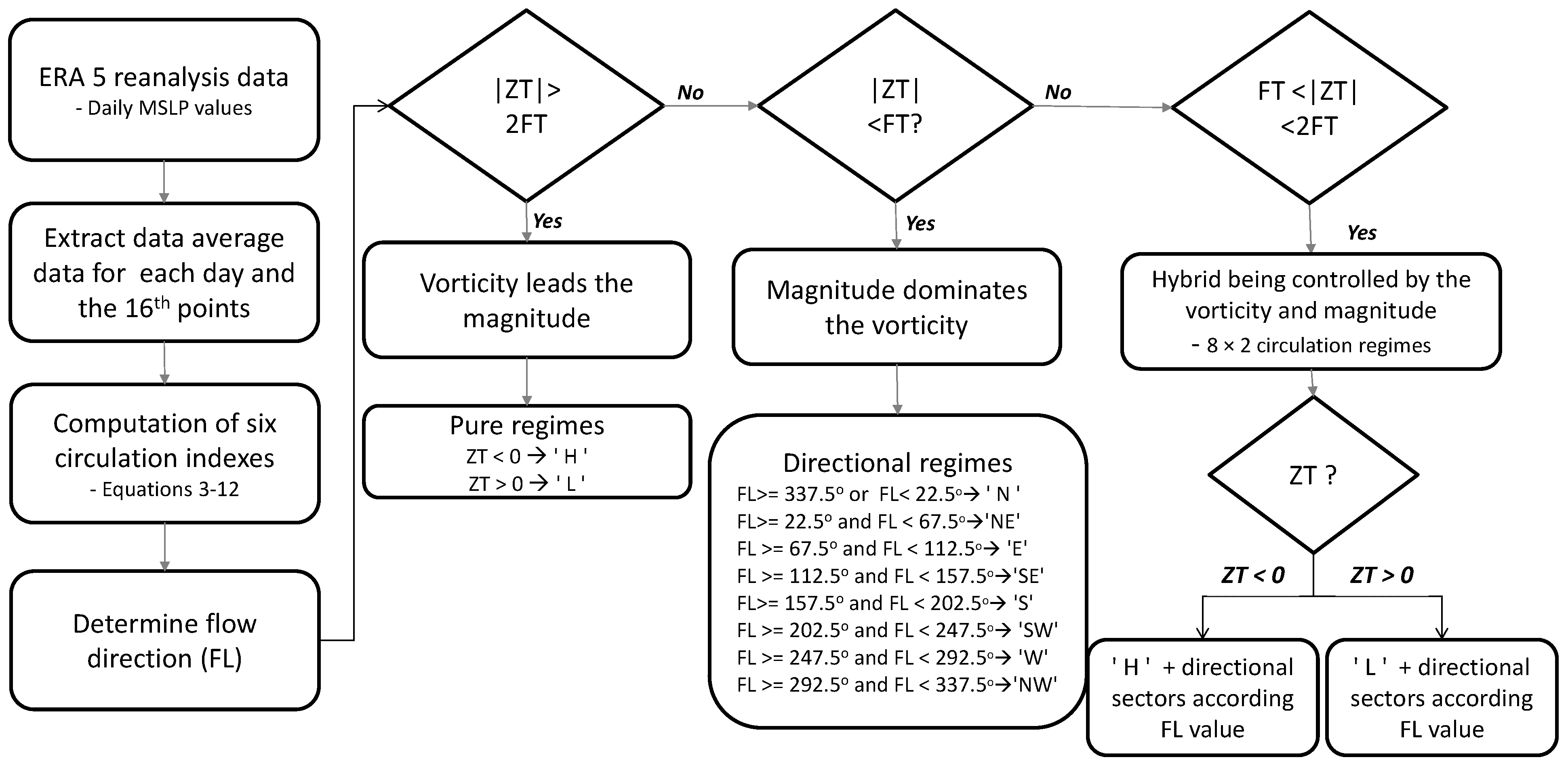
The flow direction (FL) is described by tan⁻¹ (WF/SF). In case of WF above 0, 180° were added.

-

When |ZT| < FT, the magnitude dominates the vorticity. In this case, the flow was split into eight directions (N, NE, E, SE, S, SW, W, and NW), with 45° per sector;

-

When FT < |ZT| < 2 FT, the circulation in that specific day is identified as hybrid being controlled by the vorticity and magnitude. In this case, 8 × 2 circulation regimes were considered.

-

When |ZT| > 2 FT, the vorticity leads the magnitude. If ZT is below 0, the pattern is anticyclonic (H) type. Otherwise, when ZT is above 0 it is a cyclonic (L) type.

This classification establishes a set of 26 weather circulation types (

Table 3. The 26 weather circulation types generated by the classification scheme. Adapted from [32].

Directional Sector	Anticyclonic System	Cyclonic System
N—North	H + N	L + N
NE—Northeast	H + NE	L + NE
E—East	H + E	L + E
SE—Southeast	H + SE	L + SE
S—South	H + S	L + S
SW—Southwest	H + SW	L + SW
W—West	H + W	L + W
NW—Northwest	H + NW	L + NW
	H	L

). Two of them are classified as pure anticyclonic (H) or low-pressure systems (L), eight of them are defined as directional—according to the wind rose convention—and the remaining 16 are classified as hybrid.

The main steps to implement the weather classification scheme are provided in Figure 3.

To identify the typical weather pattern for each weather circulation type, the MSLP fields for each of the 16 grid points depicted in Figure 2 were used. Considering all the days d for a specific weather circulation type, and the correspondent spatial grid points $p_{d,j}$, with j = 1, …, 16, the representative day for each weather circulation type can be obtained with the following expressions [32]:

$${\delta }_d=\mathrm{argmin} \left(\sqrt{{{\displaystyle \sum }}_{j=1}^{16}{\gamma }_{d,j}}\right)$$

(13)

$${\gamma }_{d,j}={\left(\frac{p_{d,j}-{\overline{p}}_j}{{\sigma }_{pj}}\right)}^2$$

(14)

where ${\overline{p}}_j$ and ${\sigma }_{pj}$ represent the average and the standard deviation of MSLP in the j-th point, respectively. Computing the previous equations for each day of a specific weather circulation type, the day with lowest ${\delta }_d$ can be identified and used as the closest to the climatology of this weather circulation type [32].

3. Link Weather-Type Classification with Wind Power Generation

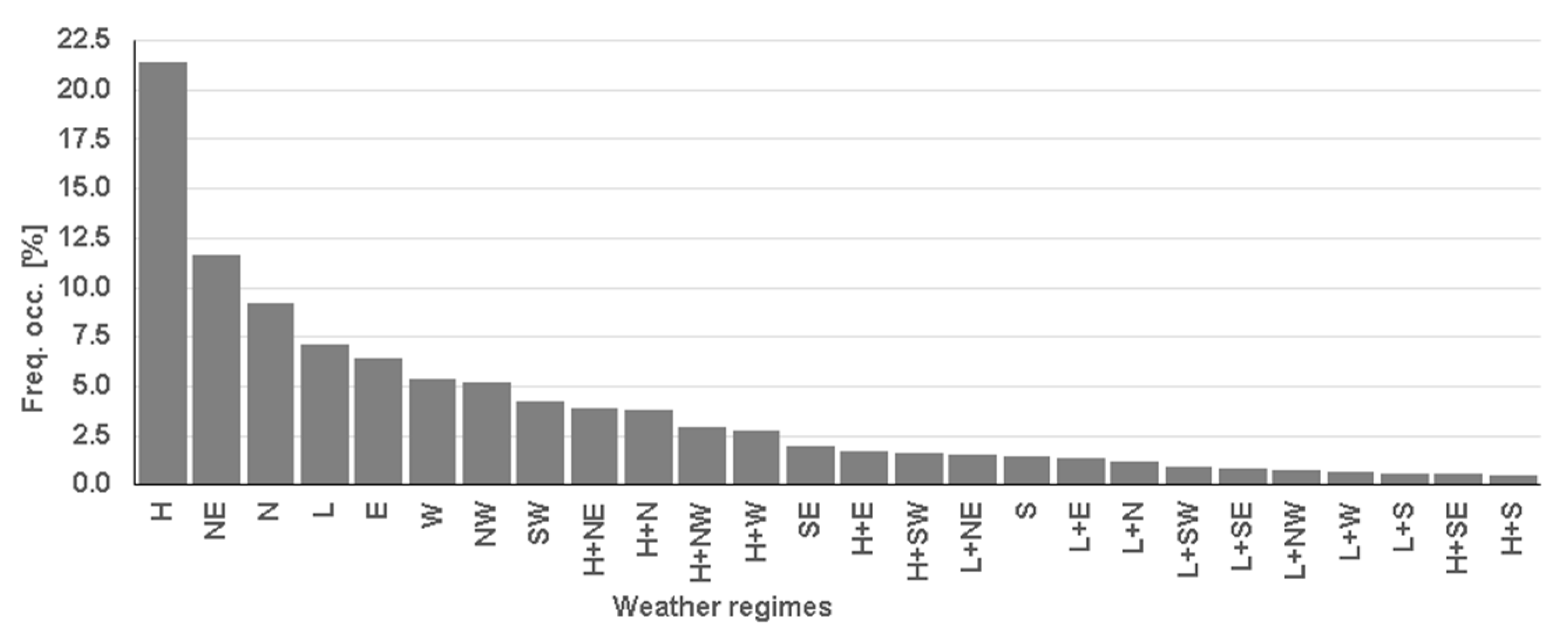
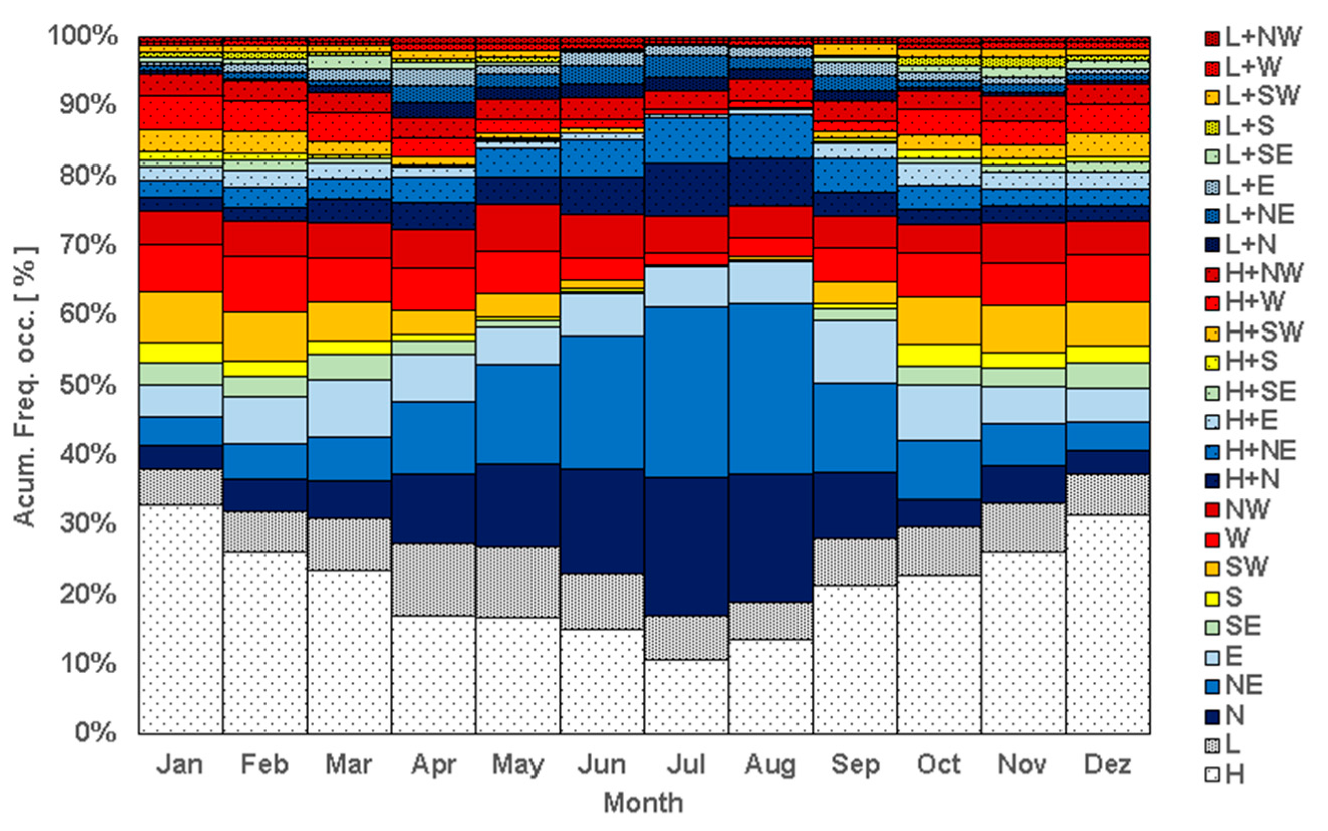
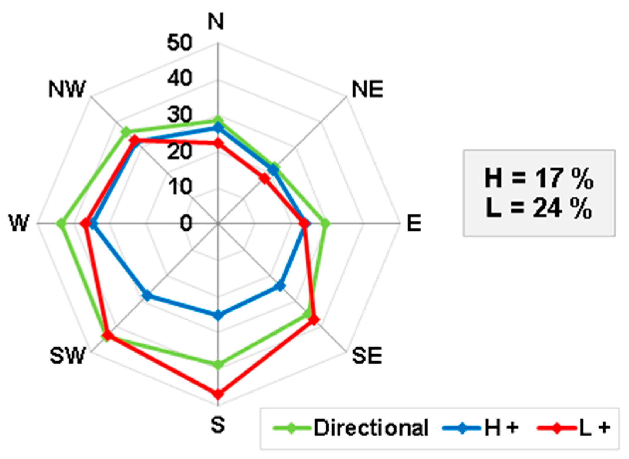
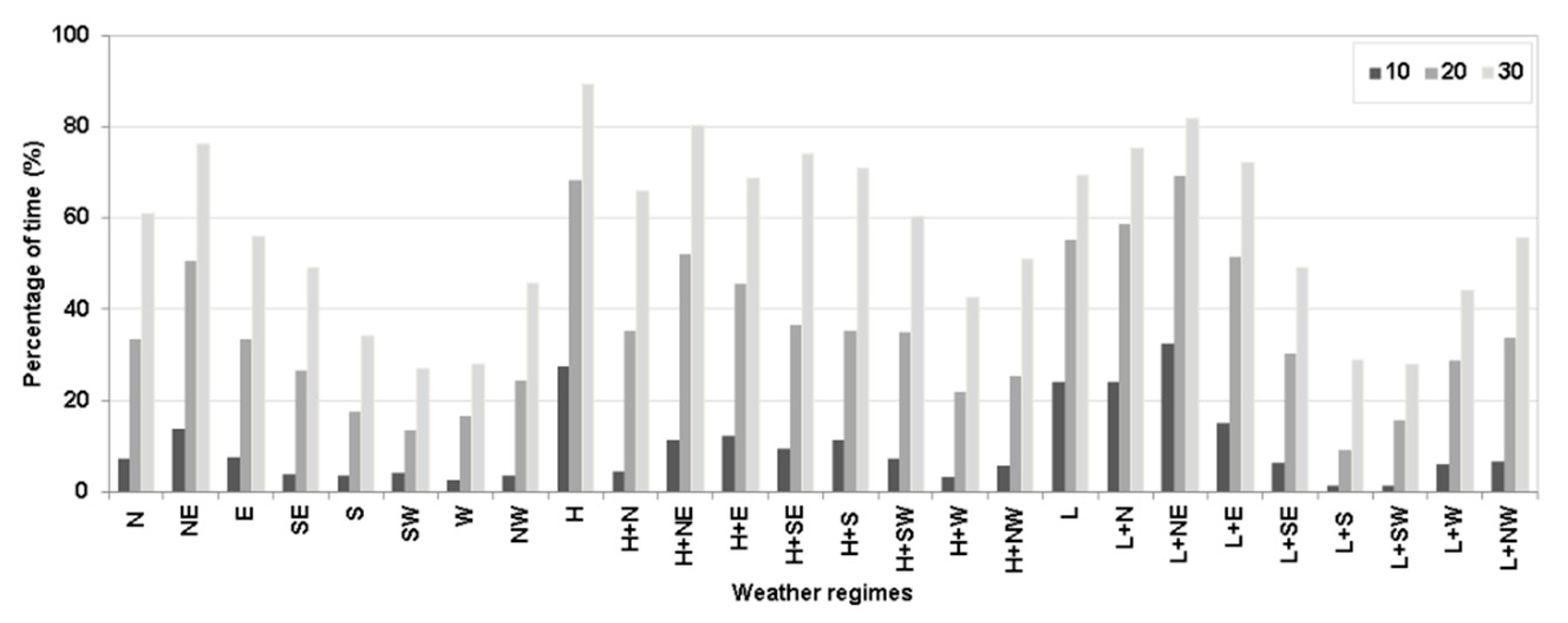
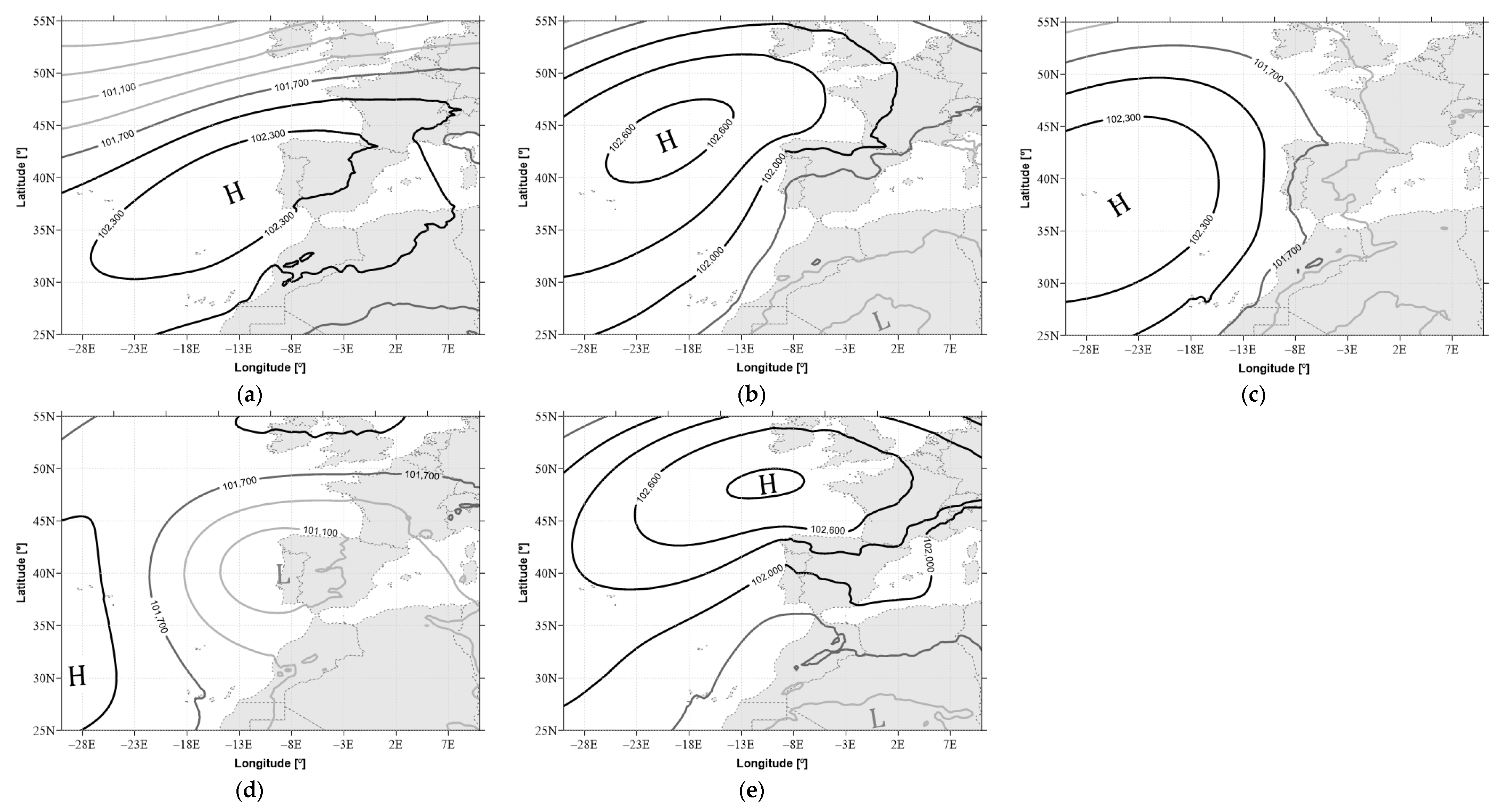
3.1. Weather Classification Type

Figure 4 depicts the frequency of occurrence of the weather circulation types during the last 70 years (1950 to 2019), and it can be concluded that the predominant weather regimes in the region under study are high-pressure system “H”, northeast circulation “NE”, and north circulation “N”. The northeast and north circulations are related to land and sea breezes, respectively.

Figure 5 depicts the frequency of occurrence of the weather regimes in consecutive 30-year periods of data compared to the total 70 years (Figure 4) and the period between 1980 and 2018, which corresponds to the long-term wind power capacity data available for this study. By splitting the dataset, it is possible to take into account the question of concept drift [9], i.e., it enables us to assess whether the weather circulation type characteristics change over time.

In a general perspective, in terms of frequency of occurrence, it is possible to conclude that the period of 1980–2018 is almost identical to the long-term data (70 years). It is also noticeable that the high-pressure system “H” increased from 1950 to 2009 and decreased after this period. The circulation regimes “NE” and “N”, associated with land and sea breezes, respectively, showed a slight increase over time, whereas the low-pressure system “L” remained constant. This same constant behavior was observed for the hybrid circulation regimes. Although the most dominant “H” regime decreased after 2009, the circulation regime “NW” increased, which represents an increase in the sea-breeze circulation from the western Atlantic coast. The typical weather regimes often associated with the occurrence of severe weather in mainland Portugal, “SW”, “W”, “S”, “L + SW”, and “L + W”, showed a small decrease over time.

Figure 6 illustrates the accumulated monthly distribution frequency of the weather regimes during the period of 1980–2018. It is visible that the “H” regime was less pronounced in the summer months and the directional sea and land breeze regimes “N” and “NW” increased in this period. The “L” regime remained constant through all the months whereas the “NW” regime notably increased over the spring months. The regimes associated with severe weather (“SW”, “W”, “S”, “L + SW”, and “LW”) tended to be more expressive in the autumn and winter months.

Figure 7 and Figure 8 illustrate the representative mean sea level pressure pattern obtained for the five most dominant weather types and for the five weather regimes that are often associated with severe weather in mainland Portugal.

3.2. Wind Power Variability

3.2.1. Daily Average Capacity Factor

The daily average capacity factor for each weather regime is depicted in Figure 9.

According to Figure 9, it is possible to verify that the capacity factor tended to be higher for pure directional regimes. The only exceptions were in the directional sectors “S” and “SE” under the influence of the cyclonic regime. The anticyclonic regimes tended to have lower capacity factors compared to pure or cyclonic regimes. The “L + S” regime presented the highest capacity factor, 46%. On the other hand, the “H” anticyclonic regime presented the lowest value, 17%. This regime had the highest frequency of occurrence (close to 22% of the time, as shown in Figure 4). The most significant difference between the regimes was found in phenomena characterized by a southern flow. “L + S” reached a capacity factor of nearly 47%, whereas the “H + S” regime presented a daily average capacity factor of 25%. On the other hand, the lowest differences were found for the northeast sector, which means that the land and sea breeze main sectors had a low impact on the daily average capacity factor.

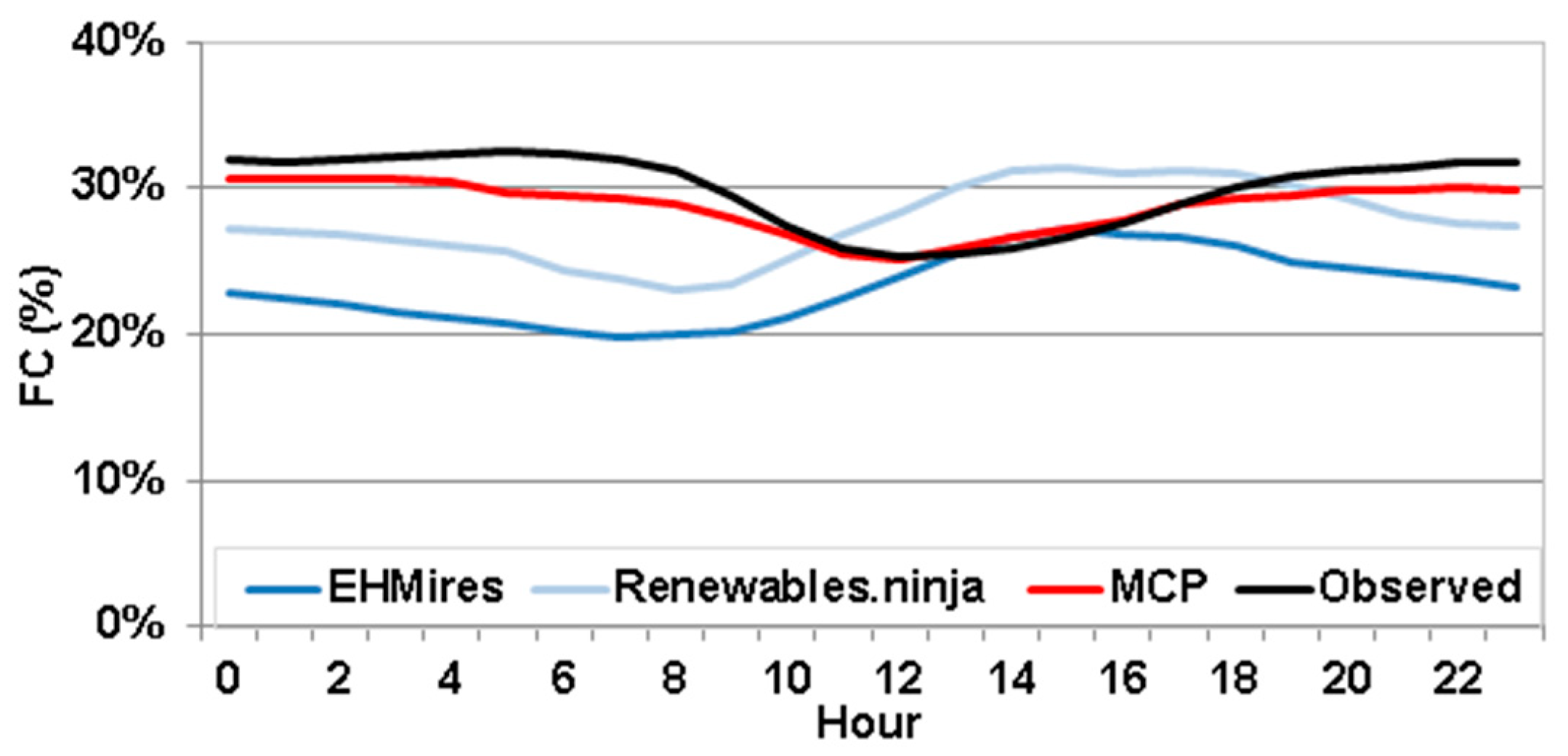
3.2.2. Wind Power Capacity Factor Daily Profile

To complement the previous analysis, Figure 10 shows the average daily profile for each regime. Knowing that the variability of the wind technology to such variations is crucial to better integrate wind power into existing systems. It can also contribute to better understanding how the generation profile of this technology can be aligned with the power demand profiles of a certain region [35].

Through Figure 10, it is possible to verify that most of the regimes had a similar generation profile, notwithstanding the different intensity. This profile, which has a “U” behavior, presented higher production values during the first hours of the day and at the end of the day, with a decrease in intensity during the first hours of the day—as can be seen in Figure 1. This behavior was more visible in all “NE”, “E”, “SE”, and “S” regimes associated with the night thermal stratification at the atmospheric boundary layer [36]. In the case of the “SW”, “W”, and “NW” regimes, the average daily profile was significantly different and there was a tendency to show the highest capacity factor during the day, associated with the daily thermal radiation development at the boundary layer. The highest daily amplitude was observed in the “E” regime; the minimum value identified was 17% and the maximum was 40%, which was reached during the first hours of the day. Contrariwise, regime “L” only showed a daily amplitude of 4%.

3.2.3. Characterization of Low-Generation Events

Low-generation events are characterized by a reduced availability of the wind resource. In this work, this analysis was performed for the different regimes by identifying the frequency of occurrence of different daily average wind power generation (Figure 11).

From Figure 11, it is possible to observe that the pure regimes “L” and “H” and the regimes from the north to the east directional sectors had a high frequency of occurrence of low-generation values. Hybrid regime “L + NE” had the highest frequency of occurrence of low-generation values below 10% of the installed capacity. According to this figure, 32% of the time, when this regime occurred, the daily average wind power generation was below 10%. This regime was closely followed by the regime “H”. These results were expected, since this regime is associated with the appearance or a development of a stable or very stable layer of atmospheric air in the boundary layer. For the “H” regime, 89% of the time the daily wind capacity factor was below 30% of the installed capacity. Extreme low-generation events were less frequent in “SW”, “W”, and “L+SW” regimes associated with an unstable atmosphere. Under these regimes, capacity factors below 20% were expected for periods less than 15% of the time. For capacity factors below 30%, the percentage of time slightly increased to 28%.

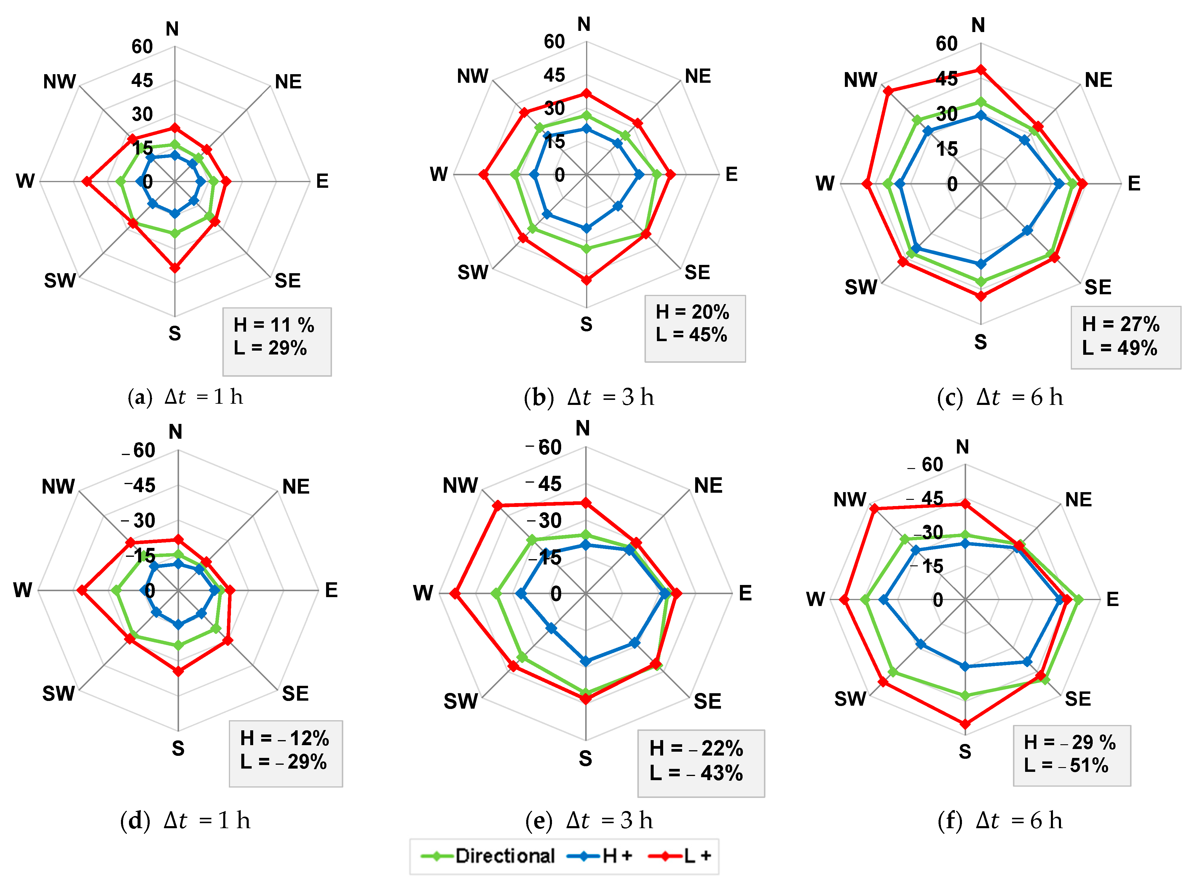
3.2.4. Characterization of Wind Power Ramps

Using Equations (1) and (2), it is possible to identify the maximum and minimum variations in each weather regime using different time intervals (Figure 12).

According to Figure 12, the “L+” regimes presented the highest variation in all directions, regardless of the time interval considered and the type of ramp (upward or downward). This result is in line with that observed in previous studies that associated the most significant ramps with atmospheric phenomena such as cyclones and windstorms [11,13]. From Figure 4 it is possible to observe that some of the most critical weather regimes presented a low frequency of occurrence. On the other hand, the “H+” regimes were the ones that present the smoothest variations.

Considering the upward wind power ramps, for the one-hour interval, the highest value (29%) occurred in the “L + W” regime, followed by the “L + S” regime. Both regimes commonly triggered convective instability to mainland Portugal, and therefore the fast upward wind power ramps are associated with convective instability. For the six-hour time interval, the directional sectors “NW” and “N” were the ones with the highest values, reaching a variation of 56% mainly caused by the sea-breeze front that detaches from the synoptic circulation due to confluence of winds that favors sea-breeze front propagation into the mountain regions. The regimes “H”, “H + NE”, and “H + E “were the ones with the smallest variation values for the different time intervals. Consequently, these regimes would be the least challenging for the TSO.

Regarding the downward wind power ramps, the behavior was very similar to that observed for upward wind power ramps. The different configurations of the cyclonic regimes were those that presented the most accentuated variations. This behavior indicates that they were also the regimes that had the highest impact, in accordance with the results verified by [11]. This means that the downward wind power ramps were affected by the presence of fast decreasing wind processes driven from the synoptic circulation such as convection inhibition up to 1 h or after the sea breeze front propagation transit up to 6 h. In a general mode, due to the wind power plant concentration in the center of Portugal, the emergence and approximation of low-pressure systems coming from the Atlantic Ocean to these regions unleashes upward wind power ramps. As these meteorological events with wind speed close to zero in the center of the system move into the interior of Portugal and cross the areas where the wind power plants are concentrated, it causes the most hazardous downward wind power ramps. In addition, the more dynamic characteristics of these systems present a high propagation speed, which makes them more quickly move away from regions where there is the presence of wind power plants. On the other hand, anticyclonic regimes are more stable and persistent in their position, presenting smooth variations in wind power production, and thus, are more predictable.

According to Figure 12, the regimes “L + SW”, “L + S”, “L + W”, and “L + NW” presented the highest variations. In these sectors, for $∆t$ equal to 1 hour the variations were above 25%, whereas for $∆t$ equal to 3 h, they reached values from 35% to 45%. For $∆t$ equal to 6 h it is possible to observe that the directional weather regimes “NE”, “E”, and “SE” presented variations above the values observed for the cyclonic weather regime. Indeed, for these directional sectors in the downward wind power ramps case, the values for anticyclonic and cyclonic weather conditions were very similar.

4. Conclusions

In this study, a characterization of wind energy generation in Portugal, with an emphasis on extreme events, was carried out using a long-term series (1980 to 2018) and a weather classification-type methodology. A Lamb-based classification method was adapted for the case study and a climatological analysis was presented. It was possible to conclude that the most common weather regime (“H”) increased its frequency of occurrence from 1950 to 2009 but showed a slight reduction in its frequency of occurrence in the last decade—from 2010 to 2019.

The hybrid cyclonic pressure system with a southern flow direction (“L + S”) regime was the one that triggered the high-capacity factor, rather than the pure directional regimes. On the other hand, the anticyclonic regimes tended to have the lowest capacity factors. From 1950 to 2019, the “L + S” regime showed a slight decrease in its occurrence over time, and the same conclusion can be inferred for the hybrid anticyclonic regimes.

Regarding the analyzed extreme events, severe variations in wind power generation were expected under the cyclonic regimes (“L+”) for any directional sector, regardless of the time interval considered and the type of ramp (upward or downward). The most severe wind power variations in a one-hour interval were observed for the “L + W” regimes, whereas for six hours they were expected under the “L + NW” regime. The maximum value identified for the upward ramp was 56%, whereas for the downward ramp the maximum was 57%. Severe variations at 1 h for upward ramps tended to be driven by convective instability from synoptic circulation into mainland Portugal, whereas downward ramps were associated with convective inhibition surgency due to the development of stable or very stable atmospheric layers. Six-hour ramps, both upward or downward, tend to be explained, respectively, by the strength or weakness of the synoptic circulation or by the transit or “after passing” of frontal systems, respectively, which propagate towards mountain regions. The anticyclonic regimes induce less variability in the wind power and therefore were less challenging for the transmission system operator.

The north-to-east directional sectors and the pure “L” and “H” regimes were likely to unleash low generation events. Regime “H” was the one with a high frequency of occurrence of low generation values, below 30% of installed capacity, due to the fact that “H” regimes tend to generate a large and stable atmosphere. During 88% of the time when this regime occurred, the daily average wind power generation was below 30%.

Since wind generation cannot be dispatched and fully controlled like conventional power plants (e.g., thermal or hydropower plants) the assessment of extreme events and the underlying role of weather regimes in triggering these events as performed in this study is crucial. This approach, which can be adapted for other regions, can enable the predictability of extreme events to be improved and power system operators to be supported, especially with a high penetration of this technology, as expected in forthcoming years, in order to decarbonize the power system and society.

References

1. Hansen, K.; Breyer, C.; Lund, H. Status and perspectives on 100% renewable energy systems. Energy 2019, 175, 471–480. [Google Scholar] [CrossRef]
2. European Comission. National Energy and Climate Plans. Available online: https://ec.europa.eu/info/energy-climate-change-environment/implementation-eu-countries/energy-and-climate-governance-and-reporting/national-energy-and-climate-plans_en (accessed on 4 May 2021).
3. Raynaud, D.; Hingray, B.; François, B.; Creutin, J.D. Energy droughts from variable renewable energy sources in European climates. Renew. Energy 2018, 125, 578–589. [Google Scholar] [CrossRef]
4. Blanco, H.; Faaij, A. A review at the role of storage in energy systems with a focus on Power to Gas and long-term storage. Renew. Sustain. Energy Rev. 2018, 81, 1049–1086. [Google Scholar] [CrossRef]
5. Gallego-Castillo, C.; Cuerva-Tejero, A.; Lopez-Garcia, O. A review on the recent history of wind power ramp forecasting. Renew. Sustain. Energy Rev. 2015, 52, 1148–1157. [Google Scholar] [CrossRef] [Green Version]
6. Drücke, J.; Borsche, M.; James, P.; Kaspar, F.; Pfeifroth, U.; Ahrens, B.; Trentmann, J. Climatological analysis of solar and wind energy in Germany using the Grosswetterlagen classification. Renew. Energy 2021, 164, 1254–1266. [Google Scholar] [CrossRef]
7. Liu, F.; Li, R.; Dreglea, A. Wind Speed and Power Ultra Short-Term Robust Forecasting Based on Takagi–Sugeno Fuzzy Model. Energies 2019, 12, 3551. [Google Scholar] [CrossRef] [Green Version]
8. Han, L.; Qiao, Y.; Li, M.; Shi, L. Wind Power Ramp Event Forecasting Based on Feature Extraction and Deep Learning. Energies 2020, 13, 6449. [Google Scholar] [CrossRef]
9. Zhukov, A.V.; Sidorov, D.N.; Foley, A.M. Random Forest Based Approach for Concept Drift Handling. In Communications in Computer and Information Science; Springer: Cham, Switzerland, 2017; Volume 661, pp. 69–77. ISBN 9783319529196. [Google Scholar]
10. Zhang, J.; Cui, M.; Hodge, B.M.; Florita, A.; Freedman, J. Ramp forecasting performance from improved short-term wind power forecasting over multiple spatial and temporal scales. Energy 2017, 122, 528–541. [Google Scholar] [CrossRef] [Green Version]
11. Couto, A.; Costa, P.; Rodrigues, L.; Lopes, V.V.; Estanqueiro, A. Impact of Weather Regimes on the Wind Power Ramp Forecast in Portugal. IEEE Trans. Sustain. Energy 2015, 6, 934–942. [Google Scholar] [CrossRef]
12. Correia, J.M.; Bastos, A.; Brito, M.C.; Trigo, R.M. The influence of the main large-scale circulation patterns on wind power production in Portugal. Renew. Energy 2017, 102, 214–223. [Google Scholar] [CrossRef]
13. Lacerda, M.; Couto, A.; Estanqueiro, A. Wind Power Ramps Driven by Windstorms and Cyclones. Energies 2017, 10, 1475. [Google Scholar] [CrossRef] [Green Version]
14. NCEP/NCAR NCEP/NCAR Global Reanalysis Products, 1948–Continuing. Available online: https://data.ucar.edu/dataset/ncep-ncar-global-reanalysis-products-1948-continuing1 (accessed on 12 July 2019).
15. Berrisford, P.; Dee, D.P.; Poli, P.; Brugge, R.; Fielding, K.; Fuentes, M.; Kallberg, P.; Kobayashi, S.; Uppala, S.; Simmons, A. The ERA-Interim Archive Version 2.0.; ERA Report Series; ECMWF: Reading, UK, 2011; p. 23. [Google Scholar]
16. Gelaro, R.; McCarty, W.; Suárez, M.J.; Todling, R.; Molod, A.; Takacs, L.; Randles, C.A.; Darmenov, A.; Bosilovich, M.G.; Reichle, R.; et al. The Modern-Era Retrospective Analysis for Research and Applications, Version 2 (MERRA-2). J. Clim. 2017, 30, 5419–5454. [Google Scholar] [CrossRef]
17. NCEP/DOE NCEP/DOE Reanalysis 2 (R2). Available online: https://psl.noaa.gov/data/gridded/data.ncep.reanalysis2.html (accessed on 12 July 2019).
18. Saha, S.; Moorthi, S.; Wu, X.; Wang, J.; Nadiga, S.; Tripp, P.; Behringer, D.; Hou, Y.-T.; Chuang, H.; Iredell, M.; et al. NCEP Climate Forecast System Version 2 (CFSv2) 6-hourly Products. Res. Data Arch. Natl. Cent. Atmos. Res. Comput. Inf. Syst. Lab. 2011, 10, D61C1TXF. [Google Scholar]
19. Couto, A.; Silva, J.; Costa, P.; Santos, D.; Simões, T.; Estanqueiro, A. Towards a high-resolution offshore wind Atlas—The Portuguese Case. IOP Conf. Ser. J. Phys. Conf. Ser. 2019, 1356, 14. [Google Scholar] [CrossRef]
20. Baumgartner, J.; Gruber, K.; Simoes, S.G.; Saint-Drenan, Y.M.; Schmidt, J. Less information, similar performance: Comparing machine learning-based time series ofwind power generation to renewables.ninja. Energies 2020, 13, 2277. [Google Scholar] [CrossRef]
21. Staffell, I.; Pfenninger, S. Using bias-corrected reanalysis to simulate current and future wind power output. Energy 2016, 114, 1224–1239. [Google Scholar] [CrossRef] [Green Version]
22. González-Aparicio, I.; Zucker, A.; Careri, F.; Monforti, F.; Huld, T.; Badger, J. EMHIRES Dataset. Part I: Wind Power Generation European Meteorological Derived HIgh Resolution RES Generation Time Series for Present and Future Scenarios; European Comission: Brussels, Belgium, 2016. [Google Scholar]
23. González-Aparicio, I.; Monforti, F.; Volker, P.; Zucker, A.; Careri, F.; Huld, T.; Badger, J. Simulating European wind power generation applying statistical downscaling to reanalysis data. Appl. Energy 2017, 199, 155–168. [Google Scholar] [CrossRef]
24. Couto, A. Creating a Wind Power Long-Term Time Series for Portugal—A MCP Approach; LNEG Internal Technical Report; LNEG: Amadora, Portugal, 2020; p. 12.
25. Freedman, J.; Markus, M.; Penc, R. Analysis of West Texas Wind Plant Ramp-Up and Ramp-Down Events; AWS Truewind Report; AWS Truewind LLC: Albany, NY, USA, 2008; p. 28. [Google Scholar]
26. Ohlendorf, N.; Schill, W.-P. Frequency and duration of low-wind-power events in Germany Environmental Research Letters Frequency and duration of low-wind-power events in Germany. Environ. Res. Lett. 2020, 15, 13. [Google Scholar] [CrossRef]
27. Philipp, A.; Bartholy, J.; Beck, C.; Erpicum, M.; Esteban, P.; Fettweis, X.; Huth, R.; James, P.; Jourdain, S.; Kreienkamp, F.; et al. Cost733cat—A database of weather and circulation type classifications. Phys. Chem. Earth Parts A B C 2010, 35, 360–373. [Google Scholar] [CrossRef]
28. Huth, R.; Beck, C.; Philipp, A.; Demuzere, M.; Ustrnul, Z.; Cahynová, M.; Kyselý, J.; Tveito, O.E. Classifications of atmospheric circulation patterns: Recent advances and applications. Ann. N. Y. Acad. Sci. 2008, 1146, 105–152. [Google Scholar] [CrossRef] [PubMed]
29. Jones, P.D.; Harpham, C.; Briffa, K.R. Lamb weather types derived from reanalysis products. Int. J. Climatol. 2013, 33, 1129–1139. [Google Scholar] [CrossRef]
30. Schyska, B.U.; Couto, A.; von Bremen, L.; Estanqueiro, A.; Heinemann, D. Weather dependent estimation of continent-wide wind power generation based on spatio-temporal clustering. Adv. Sci. Res. 2017, 14, 131–138. [Google Scholar] [CrossRef] [Green Version]
31. Jenkinson, A.F.; Collinson, B.P. An initial climatology of gales over the North Sea. Synop. Climatol. Branch Memo. 1977, 62, 18. [Google Scholar]
32. Costa, P.; Estanqueiro, A.; Miranda, P. Building a wind atlas for mainland Portugal using a weather type classification. In Proceedings of the European Wind Energy Conference, Athens, Greece, 27 February–2 March 2006; pp. 2081–2089. [Google Scholar]
33. Trigo, R.; da Camara, C.C. Circulation weather types and their influence on the precipitation regime in Portugal. Int. J. Climatol. 2000, 20, 1559–1581. [Google Scholar] [CrossRef]
34. Ramos, A.M.; Cortesi, N.; Trigo, R.M. Circulation weather types and spatial variability of daily precipitation in the Iberian Peninsula. Front. Earth Sci. 2014, 2, 1–17. [Google Scholar] [CrossRef] [Green Version]
35. Couto, A.; Estanqueiro, A. Exploring Wind and Solar PV Generation Complementarity to Meet Electricity Demand. Energies 2020, 13, 4132. [Google Scholar] [CrossRef]
36. Emeis, S. Current issues in wind energy meteorology. Meteorol. Appl. 2014, 21, 803–819. [Google Scholar] [CrossRef]
Figure 1. Daily average wind power capacity factor during January 2014 and December 2015. Adapted from [24].
Energies 14 03944 g001
Figure 2. Sea level surface pressure points and central latitude point “x” used to identify and classify the weather circulation types.
Energies 14 03944 g002
Figure 3. Flowchart of the main steps implemented for the weather regime classification.
Energies 14 03944 g003
Figure 4. Weather circulation types—frequency of occurrence from 1950 to 2019 (70 years).
Energies 14 03944 g004
Figure 5. Weather circulation type frequency of occurrence by consecutive 30-year period of data (1950–1979, 1960–1989, 1970–1999, 1980–2009, 1990–2019), the total period of 70 years of data, and the period of observational wind power capacity data (1980–2018).
Energies 14 03944 g005
Figure 6. Monthly accumulated frequency of weather circulation types for the period between 1980 and 2018.
Energies 14 03944 g006
Figure 7. Mean sea level pressure (Pa) contour maps representative of the five most dominant weather circulation types over the region under study for the period from 1980 to 2018: (a) “H”—high pressure (anticyclonic), (b) “NE”—northeast circulation, (c) “N”—north circulation, (d) “L”—low pressure, and (e) “E”—east circulation. The contour lines are gradational by color (grey—low-pressure areas, black—high-pressure areas) and equally spaced by 300 (Pa). The letters H and L in all images identify the center with high- or low-pressure values.
Energies 14 03944 g007
Figure 8. Mean sea level pressure (Pa) contour maps representative of the most dominant weather circulation types over the region under study often associated with severe weather in mainland Portugal. Period from 1980 to 2018: (a) “SW”—southwest circulation, (b) “W”—west circulation, (c) “S”—south circulation, (d) “L + SW”—hybrid low pressure with southwest circulation, and (e) “L + W”—hybrid low circulation with west circulation. The contour lines are gradational by color (grey—low-pressure areas, black—high-pressure areas) and equally spaced by 300 (Pa). The letters H and L in all images identify the center with high- or low-pressure values.
Energies 14 03944 g008
Figure 9. Average daily capacity factor according to the different weather regimes. The pure weather regimes “H” and “L” are also represented.
Energies 14 03944 g009
Figure 10. Average hourly wind power capacity factor (%) according to the different weather regimes.
Energies 14 03944 g010
Figure 11. Percentage of events with low generation (below 10%, 20%, and 30% of the total installed capacity).
Energies 14 03944 g011
Figure 12. (ac) Upward and (df) downward wind power ramps for the different weather regimes and time intervals— t (1, 3, and 6 h).
Energies 14 03944 g012