1. Introduction
Following the recent changes in the power system development, several new components entered the electricity utilization industry. Among them, electric vehicles (EVs) are expected to introduce substantial changes in the system operation and energy trading. EVs, although primarily serving as the means of transportation, can be seen as electric storages with stochastic availability. The value of the storages to the power system with an increasing amount of variable and unpredictable generation is essential [
1,
2,
3]. Development and valuation of the framework for utilization of these storages are two basic issues and this paper addresses it.
It is useful to recognize the major benefits of storages in modern power systems. Depending on the size and the type of the storage, the available flexibility can be used for the exploitation of the variations in electricity prices on different temporal scales [
4]. This rather obvious benefit has been recognized in early days of electric energy utilization and the hydro reservoirs, and the hydro-pumped plants were used for this purpose. Recently, with the increase in renewable generation presence, the necessity for short-term balancing of the variations in renewable generation emerged. In this sense, both the issue of variability and the uncertainty have to be addressed and the storages provide a suitable solution for this problem [
5,
6]. Finally, the storages can provide numerous ancillary services (frequency control [
7,
8], voltage control [
9], congestion management [
10,
11], etc.) and gain profits accordingly.
The second important question is how EVs fit into this context. Obviously, the EV storages primarily power the vehicles for transportation while the interaction with the rest of the power system occurs when an EV owner recharges the storage. In this sense, EVs can be seen as storages with stochastic availability related to human commuting habits. With aggregation, EV storage flexibility and availability increases as well as the opportunities for exploitation of the same. One part of this paper is focused on this issue where we attempt to understand how this aggregation affects the overall EV availability. In the second part of the paper a modeling framework for analysis of economic benefits of exploitation of EV fleets in renewable generation portfolios is presented. A term market aggregator (MA) emerged in this context for describing the entity performing an EV fleet related trading. Market aggregator is an agent that aggregates smaller electric market subjects (EVs) into a single subject and interacts with system operator [
12]. From the system operator’s perspective, the aggregator is seen as a large source of generation or load, which could provide ancillary services such as spinning and regulating reserve.
Hence, the major question we want to address in this paper is how beneficial is it for a market aggregator to manage a portfolio with EVs and renewable generation. In order to answer this question it was necessary to develop several novel models which present the major contributions of this paper.
In order to exploit the EV fleet storages it is necessary to estimate the flexibility available in these storages which could be used by the MA. Since our purpose is to give an estimation of the benefits of adding EVs to an existing portfolio, we assume that MA has no historical data on the actual commuting patterns. Rather, we want to address this issue from a general perspective assuming some typical behavioural patterns in vehicle usage. The proposed model is based on sequential Monte Carlo simulation which yields different EV fleet parameters used for the estimation of these benefits. The model is general and the required input data are typically available.
Once the flexibility in the EV fleet has been estimated, it is necessary to establish a suitable contractual agreement for its exploitation. In this paper we follow three agreements proposed in [
13] that the MA and the EV owner can form. This step is essential in the transformation of this concept from a theoretical to a practical one.
Finally, with the estimates on EV fleet flexibility and terms of agreements, a stochastic optimization can be applied for modeling the decision making on day ahead and sub-daily trading. When accumulated, these costs can be compared to a benchmark and the corresponding benefits can be evaluated. We apply the presented framework on different case studies emphasizing different factors regarding the fleet or an agreement.
The integral part of the model we propose is the management of an EV fleet. This issue has been investigated intensively recently. In relation to our work we would like to emphasize [
14,
15,
16]. All these papers capture the management problem while taking into account the market opportunities. However, Reference [
14] focuses on a single market, neglecting the opportunities in other markets. In [
15], authors propose a management model which takes different markets into account. However, the model is not suitable for the environment we consider for different reasons. First, decision making for a renewable portfolio with an EV fleet managed by a market aggregator differs from that of an EV fleet. Secondly, the aim of the model presented in [
15] is real-time management, while we focus on a long-term estimation of the trading benefits. The model presented in [
16] assumes a multi-market organization for a system with renewable generation and storage but considers a classic storage. Therefore, we present a novel model which assumes a multi-market scheduling of a renewable portfolio with an EV fleet from the MA’s perspective. It is also important to emphasize that the model follows a typical European market organization.
The following items summarize the contributions of this paper:
A novel Monte Carlo based model for stochastic characterization of the EV driving/charging patterns
Multi-market EV fleet scheduling model based on the virtual storage. The model considers different agreements
An estimation of the benefits of adding EVs to a renewable portfolio for MA (or Power supplier) under different agreements
The paper contents can be briefly described as follows: The first part of the first section gives a description of the contracts that the market aggregator and an EV owner can form. Through the first section, a stochastic parameter modeling approach is presented in a general context, as well as in the terms of each individual stochastic parameter used in the proposed model. Within this section, a particular focus is given to the modeling of EV-fleet-related parameters. The second section provides the model for calculation of the contract value. Finally, in the last section, the proposed model is validated through a representative case study. Furthermore, this section provides a comparison of different contracts for different fleet sizes.
2. Modeling Approach
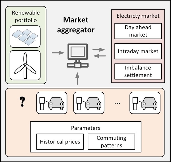
The purpose of this model is to provide a framework for the estimation of the benefits of adding EVs to the existing portfolios managed by a market aggregator. Since this estimation will be performed prior to the actual integration of the EVs, it is assumed that the data on EV patterns is unavailable unlike the data on existing portfolio performance. Overview of the complete model is depicted in
Figure 1. The model comprises two components, the simulation of the stochastic parameters and the simulation of the trading. The first component includes the simulation of the EV event dynamics and the simulation of market and portfolio parameters. These two sets of data form a complete set of parameters which, after being subjected to the scenario reduction, serve as an input to the trading simulation component.
The input data used in the model are:
Commuting patterns (distribution of daily commuting habits)
Historical portfolio data (Residual consumption, forecast error, etc.)
Historical market data (Day ahead prices, intraday prices, etc.)
Finally, the terms of agreement have to be specified and incorporated in the trading simulation. We will reduce the broad range of possible agreements to three types. The following subsection gives a detailed description of these contracts. The result of the model is a measure of the contract value. As a representative measure, we use a discount that could be given to the EV owners or the whole portfolio as a result of the savings earned with the virtual storage of the EV fleet.
Contract Specification
The benefits of exploiting EV storages shown in this paper are related to any EV fleet being managed by a single MA (also managing renewable generation). The fleet could be composed out of EVs owned by individuals or an entire fleet could be owned by a single company. The second important assumption is that this service is provided through the charger interface. If the EV is charged by the charger with no interface to MA, the terms of the contract will not be applied.
The first type of contract is denoted as Traditional. In this contract, the charging process starts when the vehicle connects to a charger. Charging is performed with the maximal available power until the vehicle is fully charged. In traditional power systems, this contract corresponds to the contract between the power supplier and a passive load. The market aggregator performs the demand forecast and buys the power on the market.
In the second contract type (denoted as Flexible), the market aggregator can exploit the storage flexibility and shift the load. However, this form of contract assumes one-direction power-flow charging stations.
In the third contract type (denoted as Prosumer), bi-directional power-flow charging stations are assumed.
The available flexibility in a
Flexible/Prosumer contract has to be constrained through several terms of agreement. The following procedure is assumed. The EV owner connects to the charging station and sets the required level of the state-of-charge and the time of departure. This requirement has to be met by the market aggregator. If the EV is disconnected from the charging station before the set departure time, the EV is left with the state-of-charge at that moment and the aggregator loses the storage. Additional terms can be set in order to enable a minimal state-of-charge for emergency car usage. A graphical depiction of the proposed contacts is given in
Figure 2 with possible power/energy trajectories. Each subfigure is related to the presented contracts. The gray area represents the availability of the storage and the maximal charging power/state-of-charge. In each subfigure, charging power
P (bars) and the State-of-charge
(line) are displayed.
3. Stochastic Parameter Modeling
According to
Figure 1, the three main components in the Stochastic parameters simulation are the EV dynamics, the Market/Portfolio data and the scenario reduction. This section gives a detailed description of these components.
3.1. EV Event Dynamics
The problem of EV related events simulation has been an omnipresent topic in recent publications. In the Introduction, an overview of the existing EV events models has been given and, here, we adopt a Monte-carlo based simulation.
At the core of this model, a single vehicle is modeled following the typical human habits. This single EV simulation model is the basic component in a general Monte-carlo model for the simulation of an entire EV fleet. The specific data to be simulated with this model have to emulate a virtual storage. The necessary data for this emulation together with those for the Traditional case are:
Charging power for the “Traditional” contract ()
Virtual storage bounds-Available minimal/maximal virtual storage capacity () and available minimal/maximal charging power ()
Departure/Arrival of the virtual storage energy ()
3.1.1. Charging Power for “Traditional contract”
In order to simulate this data for an entire EV fleet it is necessary to model them for a single vehicle. In the case of the “Traditional” contract, the vehicle is charged with the maximal available charging rate upon connection to the charging station until the maximal capacity is reached or the vehicle is disconnected. Initial condition in these dynamics is the first disconnection occurring in the morning upon departing to the workplace. This time is denoted with
for car
c and the state-of-charge at this time is assumed to be full
. The next event in the EV dynamics is the arrival at the workplace occurring at
, where
denotes the trip duration for car
c. The new state-of-charge in the moment of arrival is
, where
denotes the power used for driving car
c. The next event is determined with the availability of the charger at the workplace denoted with binary parameter
. Under the “Traditional” contract, the following charging power is used:
where
denotes the installed power of a car
c charger and
denotes the car
c battery energy content at time
t. The dynamics of the battery energy content are defined in the following:
As it is described with (
1), when the maximal energy content is reached, charging falls to zero until the departure to Home, which occurs at
. The EV arrives at Home at
with new state-of-charge
when the same charging pattern repeats through the household charger with the charging rate
and full availability:
The equations defined above describe the charging dynamics for a single vehicle, and the introduced variables are stochastic. In order to simulate an entire fleet, a Monte-carlo framework will be adopted as described later in this section.
3.1.2. Virtual Storage Bounds
In the case of “Flexible” and “Prosumer” contract, event dynamics are used for the determination of the charging flexibility. This flexibility is depicted in
Figure 3. As it was explained above, arrival at the workplace occurs at
with the new state-of-charge
. If there is a charging station at the workplace, EV owner places the planned departure time
and the desired energy content
(feasibility of the desired energy content is checked through the charging system). During the period of connection to the charging station (
), operator can charge (“Flexible”) or charge/discharge (“Prosumer”) the battery in a flexible manner (shaded area in
Figure 3), as long as the desired energy content is reached.
As it was the case with the “Traditional” contract, departure to Home occurs at and the EV arrives at Home at with the new state-of-charge when the same user specification repeats through the household charger.
The basic parameters determining the flexibility during the charging is the maximal/minimal charging rate and the energy content. Maximal charging rate is determined with:
where
T denotes the planning horizon. Minimal charging rate is defined with:
Maximal energy content
serves as an upper bound during the charging and is determined with the battery capacity. Similarly, the minimal energy content
is determined with the battery safety requirements during the connection. Both of these parameters resemble the maximal charging power determined with (
4). Instead of
and
the battery capacity
is used in the case of maximal energy content and the minimal safety state-of-charge
in the case of the minimal energy content.
The model described above covers a single EV and in order to model an entire EV fleet, a Monte-carlo based generalization can be adopted. Parameters used in the single EV model above become a stochastic parameter with its respective distribution. The sum of these parameters over an entire fleet now describes the virtual storage. Monte-carlo model of an EV fleet virtual storage is depicted in
Figure 4.
Departure times and trip duration used in the Monte-carlo model are based on analyses performed in [
17]. Trips to work or home are distributed over a day (workday or non-workday) according to
Figure 5. The first four subfigures depict the fraction of trips per each hour in the day for four characteristic trips (to work and to home for weekends and weekdays). In the fifth subfigure, the fraction of trip durations is depicted.
The battery sizes and the charger sizes are distributed according to
Table 1 and
Table 2.
Since the availability of workplace chargers varies significantly, we consider three different availability scenarios in terms of the portion of EVs having chargers at their workplaces, as depicted in
Table 3. These scenarios will provide an insight on the benefits of installing charging stations at workplaces.
The model and the data presented above are used for the simulation of EV driving/charging patterns for a fleet with 1000 and 10,000 EVs. This simulation yields the EV fleet driving patterns and the charging availability in terms of the maximal charging power and maximal storage capacity.
Figure 6 depicts these results for 1000 vehicles commuting on a single workday. In a closer examination of the first subfigure (storage power used for driving on workdays), it can be seen that the driving power increases steeply in the morning during the period of to-work commuting. The second peak occurs in the afternoon when the return to-home occurs. The second peak is more distributed due to difference in work times. The second subfigure depicts the aggregate storage availability. This value represents the aggregation of the connected storage capacities, i.e the maximal capacity of the virtual storage. During the night, all vehicles are connected to their charging station and this can be seen in the subfigure. During the morning, a steep disconnection can be noticed due to the to-work commuting. This fall is restored with the latter connection to workplace chargers in proportion to the storage availability.
Figure 6 depicts an interesting phenomenon: Even in the cases of dense commuting (workdays-to-work), just a small dispersion in commuting times can lead to a high overall availability of EV storages, assuming a high availability of the workplace chargers. In that case, storage availability has a maximal decrease of 35% for couple of hours. In cases of moderate and low availability, this decrease reaches 75%.
3.1.3. Virtual Storage Energy Arrival/Departure
In the case of the
Flexible/Prosumer agreements, it is necessary to simulate the arrival and the departure of virtual storage energy. For this purpose, we can adopt the observations presented above. Energy departure is determined with the user specified state-of-charge. Assuming that EV owners want the storages to be full by the time they go to work/home, the time-dependent user-defined energy content can be determined based on the distributions of the departures in these directions through Monte Carlo simulation, as depicted in
Figure 7. In order to determine the uncertainties in actual departure times compared to the planned ones, normally distributed random variations in departure times are simulated and superposed on these scenarios.
The arrival of virtual storage energy can be determined in the same manner as it was described for the “Traditional contract”, using .
This model is applied on the same set of vehicles used in the previous simulation.
Figure 8 depicts the results for the cases of low, mid and high availability of the workplace chargers.
3.2. Market and Portfolio Data
In this section, we give a generic mathematical simulation framework for the stochastic parameters and the deployment of this framework on each specific parameter considered in the optimization model. These stochastic parameters are:
These parameters are used for the scenario tree generation representing the uncertainties a market aggregator faces in the decision making at different stages. Three characteristic stages are: day ahead market, intraday market, and imbalance settlement. This represents the typical electricity market organization. First, the energy is traded for each hour in the next day followed by market closure before the next day starts. Once the next day is entered, market participants have the opportunity to correct their bids (typically to follow the realizations of uncertainties) for the next hour. After this stage, the real-time operation is performed. During real-time operation, the realizations differ from the bids and penalties are charged in the imbalance settlement procedure.
Secondly, it is necessary to build up a set of representative days composed of all these uncertain parameters which can then be used to estimate the annual costs. Altogether, the scenario tree corresponding to the decision-making process in a multi-market organization is depicted in
Figure 9. The complete scenario tree in
Figure 9 comprises several independent trees each related to a representative day.
The details on EV-fleet-related parameters simulation are given in the previous section. The remaining three categories of uncertain parameters are an omnipresent topic in the relevant literature, and only a brief explanation of the adopted modeling approach is given in the following text.
For the day ahead prices, a set of historical prices is used. These daily realizations are used as the basis for the superposition of the uncertain realization of the subsequent stages. These scenarios are simulated using different orders of multiplicative autoregressive integrated moving average (ARIMA) models [
18] with transformations based on the theory of Copula [
19]. Autoregressive models have been widely applied in electricity prices modeling and forecasting [
20,
21] and portfolio forecast error modeling [
22,
23,
24]. The basic idea behind autoragressive models is that each value in a series is a linear combination of past values and white noise. Based on the historical data, the parameters of such linear model are fit through optimization. On the other hand, the Copula theory allows for simulation of multivariate distributions with specific distribution types and correlation matrix. This framework allows for the simulation of different realizations of uncertain parameters forming the scenario tree.
Using the presented framework, 1000 scenarios are generated.
Figure 10 depicts these scenarios for day ahead price, intraday price, portfolio consumption and day ahead forecast error of the portfolio consumption. These scenarios, together with previously depicted fleet-related scenarios form a complete set of scenarios required in the model. These scenarios will be reduced using the reduction technique described in the following section.
3.3. Scenario Reduction
The reduction in the number of scenarios is necessary in order to reduce the computational complexity. For the same reason, it is necessary to select representative days instead of optimizing over the whole year. The scenario reduction technique presented in [
25] is adopted here. This method is based on the elimination of all the similar scenarios except for one which then takes over their probabilities. The same method can be applied for the selection of the representative days where instead of probability, the remaining day will have a greater weight in the summation of the total annual cost.
It is important to point out that in the case of EV fleet dynamics scenarios, due to the substantial differences in stochastic EV fleet parameters related to workdays/non-workdays commuting, the scenario reduction and the representative days selection is applied on these two subsets separately.
4. Portfolio Value Model
In this section, the mathematical model for estimation of the portfolio value on an annual level is presented. In the case of the Traditional contract, this value is calculated through a set of algebraic equations. Multi-stage stochastic optimization is required for portfolio value estimation in the case of Flexible and Prosumer contracts.
4.1. Traditional Contract
The estimation of
Traditional contract value is performed through the simulation of the charging scenarios and the summation of the corresponding costs at different stages. We assume that each EV is connected to a charger as soon as it reaches the destination (if the charger is available at this destination). Upon connection, the vehicle is charged with the maximal available charging rate till it reaches the full state-of-charge as it was described in the
Section 3.1.
Calculation of the total annual costs for supplying the portfolio under consideration can be done with the following expression:
with:
| the weight of scenario , |
| the day ahead/intraday electricity price, |
| the day ahead portfolio consumption/production forecast, |
| the day ahead portfolio consumption/production forecast error, |
| the imbalance determined as , |
| the imbalance price. |
If we assume the day ahead error balancing on the intraday market, the only deviations that remain are the hour-ahead deviations. Therefore, the imbalance
can be determined with:
with:
| the hour-ahead portfolio consumption/production forecast error. |
The price
in the two-price imbalance settlement procedure depends on the relation between the the portfolio error direction and the system error
direction according to
Table 4.
Different system error direction scenarios are simulated in order to capture the two-price procedure. In practice, the MA will have historical data on its portfolio error, while the data on the system error are publicly available. From this, the correlation could be determined and reproduced. Here, a correlation in error directions of 0.8 is assumed. Such a correlation could be expected since the system error is the sum of errors of all portfolios in the system including the examined portfolio. Portfolios are within certain geographical area and are correlated accordingly [
26].
Results of the portfolio cost estimation are shown in
Table 5 expressed as the cost per MWh of the actual consumed power (over the counter) for different availability of workplace chargers.
4.2. Flexible/Prosumer Contract
The model presented in the following text is the modification of the storage scheduling model proposed in [
16].
The market aggregator forecasts portfolio consumption/production and, based on these forecasts, buys/sells power on the day ahead market. We also assume the market aggregator is a balancing responsible entity. This means that the aggregator is financially penalized for mismatches in forecasts. Since our aim is to analyze the value of different contracts that the aggregator can offer to newly added electrical vehicles, it is necessary to consider this component of the portfolio separately. The three-stage stochastic optimization model describes these market operations, and a detailed description is provided in the following paragraphs.
The first stage is related to the day ahead market. The market aggregator decides the EV fleet charging/discharging power for the day ahead market
based on the expected gains determined with:
subject to:
Objective (
8) comprises the expected revenues in the day ahead market. These gains consist of the profit/cost of the residual load of the portfolio and the profit/cost for the purchase/sale of the power related to EVs. The term
denotes the revenues related to the forthcoming stages. Constraint (
9) enforces non-anticipativity.
The second stage is related to the intraday market. This market primarily serves to correct the day ahead bids. Hence, the aggregator corrects the day ahead bids on the intraday market with sales/purchases denoted with
following updates on parameter forecasts. The objective describing the expected gains/costs in the intraday market is:
subject to:
where:
Objective (
10) comprises the costs/revenues in the intraday market. The term
denotes the forthcoming trading. The term
is primarily a trading quantity and not necessarily related to physical processes. Constraint (
11) ensures non-anticipativity. Constraint (
12) ensures that the intraday market is used only for forecast error correction.
The final stage is related to the real-time operation and post-realization tradings. At this moment, the actual errors in planned vs. delivered power are known. Hence, the penalties can be charged through the imbalance settlement. On the other hand, these imbalance costs will motivate for error correction through real-time operation. This is expressed in the following objective:
In Objective (
14),
denotes the costs for imbalances charged after real-time operation. Again, the imbalance settlement procedure follows the so-called two price mechanism. The prices for different combinations in system and portfolio error directions are depicted in
Table 4. Here,
denotes the real-time portfolio imbalance (
). The following constraint captures these imbalance costs:
where:
Here, denotes the system error direction, while the the sign of shows the portfolio error direction.
The charging dynamics are captured with the following constraints:
where a new variable
represents the additional power produced in this stage relative to the preceding actions. The sum
represents the power produced/consumed in real-time. As such, it is used in the constraint (
18) and drives the Virtual storage energy dynamics. In this constraint the energy departure and arrival defined in the previous section is introduced as well. Constraints (
19) and (
20) bounds the virtual storage energy content and the real-time charging power between minimal and maximal value defined in the previous section. Constraint (
21) enforces the temporal continuity.
5. Case Study
This section provides the details on the solution of the proposed optimization problem together with the details of the case study. In the second part, three proposed contracts are analyzed.
5.1. Solution Technique and Case Study
The proposed contracts are analyzed with different workplace charger availabilities and with scenarios simulated in
Section 3. The portfolio integrates an EV fleet with 1000 vehicles, and the complete set of scenarios is reduced to 10 × 5 × 20 scenarios for three stages.
The presented optimization model is modeled in Python and solved with GUROBI solver [
27]. GUROBI is a state-of-the art solver specialized for mixed-integer linear optimization problems. A python library allows for easy integration of the solver into a python programming framework.
Complete trading in a single scenario is shown in
Figure 11. Day-ahead-related trading suggests exploitation of daily price differences. The second opportunity exploited by virtual storage is the imbalance penalty avoidance. Exploitation of this opportunity is clearly depicted in
Figure 11. However, some errors remain unbalanced due to the lack of flexibility, greater gains on day ahead market, etc. The intraday market is used for day ahead error balancing, and these errors are balanced completely.
5.2. Comparative Analysis
The
Traditional contract serves as the benchmark in the comparative analysis. The
Flexible/Prosumer contracts are compared to the
Traditional with:
In this expression, the difference in portfolio supply costs under the
Flexible/Prosumer contract,
is given (form of discount) to EV owners in one case
or to the complete portfolio in the other
. The price
can be seen as a discount that can be given to the EV owners or to the complete portfolio under a certain contract and still have the same profit as in the case of
Traditional contract.
Table 6 depicts these results. In both cases of contract a significant discount can be given to the EV owners. In case of
Prosumer this discount exceeds the traditional price meaning that the supplier can pay the EV owner to supply his/her EV. On the other hand, if the benefits would be given to the complete portfolio, the possible discount is negligible. This is primarily due to the size of the fleet in comparison to the rest of the portfolio. Installing charging stations on the workplace does not increase the benefits significantly. In fact, in the case of
Flexible contract, costs for traditional charging are higher than the benefits of the contract, resulting in a slight decrease of the discount. This smaller gain is the result of the charging enforcement during the day (when the prices are higher) as a result of user-defined specifications on the departure state-of-charge when commuting to home.
In order to understand the effect of the workplace charging station availability, a probabilistic depiction of the state-of-charge can be used.
Figure 12 depicts the mean and the standard deviation of the state-of-charge trajectories in workday scenarios for a
Prosumer contract. Obvious differences in the charging patterns depict the exploitation of the available flexibility. The above mentioned increase in the departure state-of-charge prior to work-to-home commuting is visible in this depiction during afternoons.
In the comparison above it was stated that when the savings are given to the portfolio, the discount is negligible due to the size of the fleet compared to the rest of the portfolio. It is therefore useful to consider a larger EV fleet under the same contract. Assuming a
Prosumer contract and high charger availability an EV fleet of 10,000 vehicles is considered.
Table 7 shows the discounts in this and the previous case. Now, the benefits are large enough to result in a significant discount for the whole portfolio (7.1€/MWh). However, the discount given to the fleet has decreased compared to the 1000 EV fleet. This is due to the saturation effect in terms of imbalance reduction requirements. Namely, the capacity of the virtual storage exceeds the imbalance error and hence the profit in this market is completely exploited and can not be increased with the increase of virtual storage capacity.
6. Conclusions
In this paper a novel method for the estimation of the economic benefits of adding EVs to the existing renewable portfolios is given. The perspective of a market aggregator is assumed. The method is suitable for the planning stage when the actual data on vehicle commuting patterns is unavailable. Furthermore, different supply contracts have been proposed in order to set the terms of storage usage that satisfy the requirements of both an EV owner and a market aggregator.
In order to get an indicative assessment of these benefits, a realistic case study is used. It was recognized that the integration of EVs in renewable portfolios can be highly beneficial in terms of economic gains. The flexibility introduced through this integration can be used for exploitation of the price variations or for the portfolio imbalance correction. A characteristic measure of economic benefits is adopted for valuation of economic benefits: The savings on the portfolio level (compared to traditional contract) are divided with the driving energy (given to EV owners) in one case and divided with the energy of the whole portfolio (distributed over the whole portfolio) in the second case. The results show that in the case of “Flexible” contract a total amount of approx. 16 €/MWh can be given to each EV owner which is more than half the price they paid for charging. In the case of “Prosumer” contract, this amount reaches up to 57 €/MWh exceeding the price paid for charging. This means that the aggregator can pay EV owner to charge his/her vehicle. The second major conclusion drawn from the conducted analyses is the saturation effect. Namely, if the fleet size would increase, the benefits would decrease relative to the number of EVs. This effect is the consequence of the over-sized storage capacity compared to imbalance correction needs. However, the other gains still remain and the benefits are still significant. Furthermore, in the case of an increased fleet size, the benefits are large enough to result in savings for the whole portfolio.
It is important to point out that these conclusions are related to the case study under consideration and should not be used as general conclusions. Furthermore, the proposed model neglects several important factors. The cost of the charging infrastructure is not considered, and in order to get a realistic assessments of the benefits, these costs should be analyzed. The second major assumption is the neglect of the battery deterioration caused by increased cycling. However, the obtained results point to a large opportunity in combining the EVs with the renewable portfolios.
7. Model Limitations and Further Research
The basic assumption behind the EV storage exploitation is that this service is provided through the charger interface. If the EV is charged by the charger with no interface to MA, the terms of contract will not be applied. This is one of the basic limitations since it can be expected that other chargers will be used as well. However, the EV owners outside of this category (with different traveling habits) will not be motivated to sign such a contract. Furthermore, we can expect that, in the future, all charges will have such communication capabilities and these services will become a standard.
In this paper, the category of interest are commuting EVs. However, other categories of vehicles can fit this role as well. For example, delivery EVs and public transportation are interesting categories to be investigated in this context. The continuing research could cover this and other categories of vehicles.
The possibility of delivering other ancillary services could be investigated as well. For example, voltage and frequency control could be provided by EV storages and additional profit could be gained. Such research could show even greater benefits of integrating EVs in power system operations.
Finally, an important research topic in this context is the control system design for provision of services presented in this paper. Namely, these services are based on the exchange of control signals between central entity and numerous charging devices. Desired change in EV power consumption/production would have to be evenly distributed over active storages.


