1. Introduction
The rapid economic growth and industrialization of China in the past decades have been accompanied by various environmental problems, especially escalating air pollution and water contamination. While there is contention regarding the scale of and remedy for those problems, the consensus in both politics and academia is that environmental problems are posing a serious risk to sustainable development and need to be addressed immediately. The current Chinese government has vowed to make environmental protection the top priority in administration. In 2014, the Chinese government declared “war against pollution”, which marked repositioning of the long-standing policy of prioritizing economic growth over environment. Five years have passed, and there are signs that China has made steady progress in winning the war on pollution, as manifested by the remarkable improvement in air quality [
1]. Meanwhile, concerns over the detrimental effects of tightening environmental regulations on economic growth are mounting. The problem is especially pertinent at a time when the economy is growing at its slowest rate since 1990. In the most recent annual session of the congress in 2019, some local officials voiced their concerns and called for loosening up of the state environmental policies [
2].
Since China is a vast country with huge regional differences, the challenge of pollution has different effects on different regions. For instance, regions with coal-dependent economies have historical burdens of polluting industries. Limited financial resources make it particularly difficult to simultaneously meet economic and environmental targets [
2]. Despite general agreement about the importance and urgency of environmental protection, there remain a lot of controversies about the obligations that different regions should assume and the types of policies that are most appropriate in the battle against pollution. To resolve the controversies and lay the foundation for future actions, we need to have a clear understanding of what the regions have achieved in the past. To this end, this research aims to assess the sustainable development of Chinese provinces. (There are 34 provincial-level administrative divisions in China, including 23 provinces, four municipalities, five autonomous regions, and two special administrative regions. For the sake of conciseness, we refer to them as provinces throughout the article).
The assessment serves two critical purposes. First, the proposed assessment can enable us to uncover the patterns of sustainable development with environmental protection at a provincial level. Analyzing the patterns can help us assess the impact of policies on sustainable development and assist us in improving the design of environmental policies. Second, the provincial-level assessment allows us to prepare a benchmark for the provinces that is based upon their development status and geographical locations. The assessment can identify the underperforming provinces that should gear up their efforts in meeting the environmental challenge. In summary, assessing provincial-level sustainable development is an important issue that bears significant practical implications.
Methodology-wise, most sustainability assessment studies rely on defining and quantifying main performance measures and indicators, especially various types of sustainability indices. While such indices can reveal important implications, there are two primary concerns with these index-based analyses. One concern is that sustainability indices are usually based upon the ratio of a single output (e.g., pollutant emissions) to a single input (e.g., GDP), thus failing to account for other factors that are involved in shaping the sustainability. The other concern is that some indices consider more than two factors by combining the factors via weighted average method, but the weights assigned to the factors are usually artificially set and are subject to criticisms. To overcome the predicament of existing index-based analysis and adequately assess sustainability, we need a scientific, holistic and robust approach. Since economic development and environmental protection are two pillars of sustainability, this study discusses how to measure the level of sustainability in various provinces by examining their status in both economic and environmental dimensions.
This research proposes Data Envelopment Analysis (DEA) as the methodology to assess the level of sustainability. We formulate three DEA models, under the assumptions of natural disposability, managerial disposability and null-joint relationship respectively. Natural disposability assumes that a production unit can decrease its pollution by reducing production activities. Managerial disposability means that a production unit can increase its production activities and decrease pollution simultaneously by managerial efforts (e.g., green technology). The null-joint relationship specifies that pollutions are by-products of desirable outputs and do not exist without desirable outputs. We apply the three models to a sample of Chinese provinces for the period 2004–2017. The study takes the provinces’ capital stock, labor, energy use, GDP, SO2 emissions, wastewater discharge and CO2 emissions into account.
Abbreviations used in this research are summarized as follows: CO2: Carbon Dioxide, DEA: Data Envelopment Analysis, DMU: Decision Making Unit, DTS: Damages to Scale, GDP: Gross Domestic Product, MEE: Ministry of Ecology and Environment, MEP: Ministry of Environmental Protection, NOX: Nitrogen Oxide, RMB: Renminbi (i.e., Chinese currency), OECD: Organization for Economic Co-operation and Development, PM: Particulate Matter, RTS: Returns to Scale, SEPA: State Environmental Protection Administration, SGM: Sustainability Growth under Managerial disposability, SGN: Sustainability Growth under Natural disposability, SGNM: Sustainability Growth under Natural and Managerial disposability, SO2: Sulfur Dioxide, TCE: Tons of Coal Equivalent, UC: Undesirable Congestion, UE: Unified Efficiency, UEM: Unified Efficiency under Managerial disposability, UEN: Unified Efficiency under Natural disposability and URS: Unrestricted.
The rest of this study proceeds in the following manner.
Section 2 outlines the background of this research and reviews relevant work.
Section 3 presents the concepts behind this study.
Section 4 elaborates the methodologies.
Section 5 describes the data sample.
Section 6 summarizes the results.
Section 7 discusses policy implications and research limitations along with future research directions.
2. Research Background and Literature Review
Due to the delayed industrialization process, environmental protection was not a major issue in the administration of China until the second half of the 20th century. The major policies and legislations on environmental issues by China have been described in [
3]. In 1973, China set up the Environmental Protection Leadership Commission, the country’s first regulatory entity devoted to environmental issues. At that time, the environment of China was already in critical condition, which would be further exacerbated by the ensuing economic reforms. In 1978, at the eve of the so-called “reform and opening-up” [
4], China added the following statement to its constitution: “The state protects the environment and natural resources. It also prevents and controls pollution and other public hazards.” This statement provided the constitutional foundation for the country’s administration to deal with environmental problems. In the next year, 1979, the country passed the Environmental Protection Law, which required all provincial governments to set up environmental protection and supervision agencies.
The 1980s and 1990s marked the country’s widespread national administrative reforms. The Environmental Protection Leadership Commission was replaced by the Environmental Protection Agency, which was a branch of the Ministry of Urban Construction and Environmental Protection. In 1983, the government announced that protection of environment was a state policy. Later on, environmental laws were enacted, such as the Law of Air Pollution Prevention and Control of 1987, the Energy Conservation Law of 1997 and the Clean Production Promotion Law of 2002. In 1998, the government decided to upgrade the Environmental Protection Agency from a branch of a ministry to a ministry itself and named it SEPA.
During the 2000s, environmental protection played an increasingly important role in the administration of the country. As the number of mass protests caused by concerns over environmental issues grew steadily [
5], the government adopted harsher measures on environmental protection. For instance, emissions standards were raised, subsidies for some polluting industries were reduced or even cancelled, and quite a number of polluting factories were shut down [
6]. In 2004, the government launched the “Green GDP” pilot program, in which regional GDPs were adjusted to compensate for negative environmental impacts [
7]. As the promotion of officials was closely tied to GDP, it was expected that the “Green GDP” program would give the local authorities strong incentives to improve environmental performance. However, despite initial success in several provinces, the “Green GDP” program quickly lost steam after the financial crisis in 2008, because the central government backed down out of fear of an economic slowdown. In 2008, the SEPA was restructured as the MEP, which was elevated to the status of a cabinet member and endowed with greater political power. In 2018, the MEP was superseded by the MEE, which was endowed with additional responsibilities originally borne by other ministries. The establishment of the MEE demonstrated the strong political will and commitment of China’s central government to environmental protection, as well as the development of an integrated governance approach.
A major event in the country’s efforts on environmental protection came in March 2014, when the government declared “war against pollution” during the opening of the National People’s Congress [
8]. The next month, the parliament approved a new environmental law which went into effect in January 2015. The new law endows environmental protection agencies with greater punitive power and gives non-governmental environmental groups more room to operate in the country.
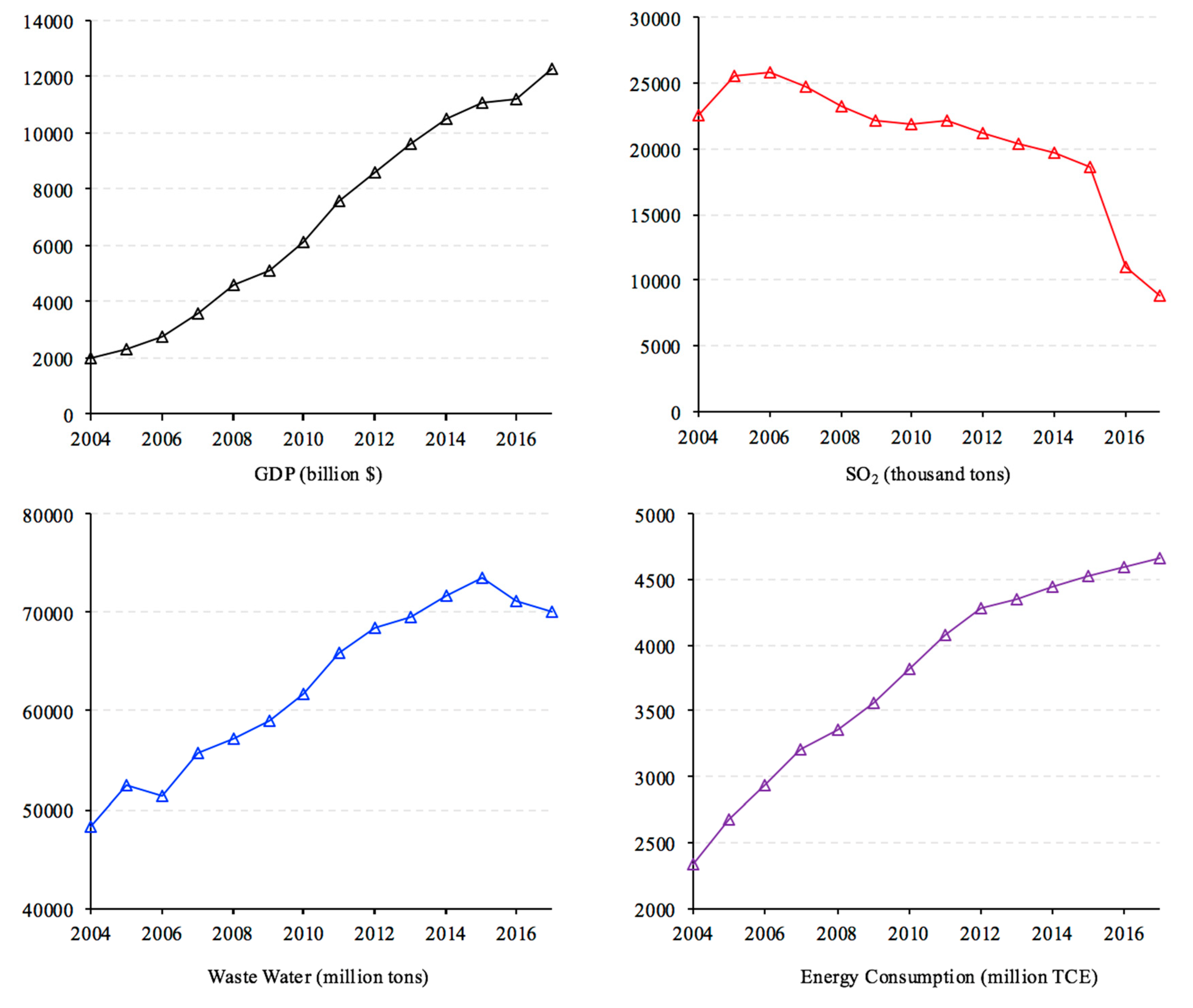
To illustrate the sustainable development of China,
Figure 1 shows the change of GDP, SO
2 emission, wastewater discharge and energy use for 2004–2017. China’s SO
2 emission peaks in 2006 and thereafter has been steadily decreasing. Wastewater discharge increases from 2004 to 2015 and the trend seems to reverse after 2015. Energy use has been steadily increasing, but the rate has shown a clear downward trend after 2012, most likely thanks to slowdown of economic growth and deployment of energy saving measures.
Our research is related to the expanding stream of literature on regional-level sustainable development [
9,
10,
11,
12,
13,
14,
15,
16]. Typically, studies in this domain explore the pattern of longitudinal economic and environmental performance. For example, Reference [
9] examines the environmental performance of OECD countries and finds that performance tends to converge for groups. Using a national data set, Reference [
14] studies the carbon intensity of human well-being and finds regional differences in terms of economic development impact the carbon intensity of human well-being. Reference [
17] studies the carbon footprints of 73 countries and 14 regions, and decompose the contribution into eight sectors. Many studies have conducted regional comparison in a time horizon. Reference [
18] discusses environmental performance analysis in a time series data set, using the Malmquist index measurement. Reference [
19] examines effects of financial development indicators on energy consumption and CO
2 emission via international comparison involving European, East Asian and Oceania countries. Reference [
20] discusses the country-level eco-efficiency measured by directional distance functions. Reference [
21] examines the dynamics of eco-efficiency of countries in the European Union.
A plethora of studies have zoomed in on the regional and provincial sustainable development of China. Reference [
22] constructs the total-factor energy efficiency indices for 29 administrative regions in China during the period 1995–2002, and find that energy efficiency improves with economy. Reference [
23] computes the three industrial waste abatements for 30 regions in China and finds that the east area contains most of the efficient regions. Reference [
24] derives Malmquist indices to assess the effects of three factors (economic structure, energy consumption structure, and technological progress) on energy intensity. Reference [
25] measures China’s regional integrated energy and environmental efficiency over 2006–2010 using DEA under the concepts of natural disposability and managerial disposability. Reference [
3] examines China’s regional economic performance and air pollution based on simulated PM2.5 and PM10 emissions.
Position of this study: The previous studies have employed various statistical and econometric modeling techniques to analyze the sustainable development at the national level, including general equilibrium models, panel data regression, input–output analysis and time series analysis. Specifically, various mathematical programing approaches including DEA have been proposed to compute the level of efficiency-based sustainability assessment. See Reference [
26] for a comprehensive literature survey in this respect. This study is, methodologically, an extension of the previous studies on DEA environmental assessment. As specified in the survey [
26], no studies have clearly explored a use of DEA for enhancing Chinese sustainability under the assumption of a null-joint relationship. It is envisioned that the proposed study produces new empirical results which we cannot obtain by the conventional methods.
3. Underlying Concepts
This section describes three concepts used for developing three sustainability growth indices under the DEA framework.
3.1. Production Factors
Figure 2 depicts the relationship among three production factors (
X: an input vector,
G: a desirable output vector and
B: an undesirable output vector). As depicted in
Figure 1, all DMUs uses
X to produce
G. The production of
G is usually associated with
B. Thus,
B is “by-products” of
G, both of which are originated from the utilization of
X. The more
G and less
B produced, the better the performance in this assessment. The relationship is referred to as the “null-joint hypothesis”.
3.2. Disposability Concepts
To adapt the conceptual discussion in
Figure 2 to DEA formulations for environmental assessment, we need to utilize the concepts of “natural disposability” and “managerial disposability”.
X denotes an input vector of
m elements with positive real values.
G is an output vector of
s desirable elements.
B is an output vector of
h undesirable elements. In these vectors, the subscript (
j) is used to represent the
j-th DMU. Here,
R stands for a vector of real numbers. The superscript indicates the dimension of each vector, and the subscript implies that all the components are strictly positive.
The unified production possibility sets to express natural disposability (
N) and managerial disposability (
M) are as follows:
stands for a production and pollution possibility set under natural (N) disposability. Meanwhile,
is for managerial disposability.
A difference between them is that the production technology under natural disposability, or , satisfies , such that a DMU can move toward the efficiency frontier by decreasing X. In contrast, the production technology under managerial disposability, or , has , implying that a DMU can attain efficiency by increasing X. A common feature of the two concepts is that both have and . The two conditions on G and B are acceptable, because an efficiency frontier for G should locate above or on all DMUs, while that of B should locate below or on them.
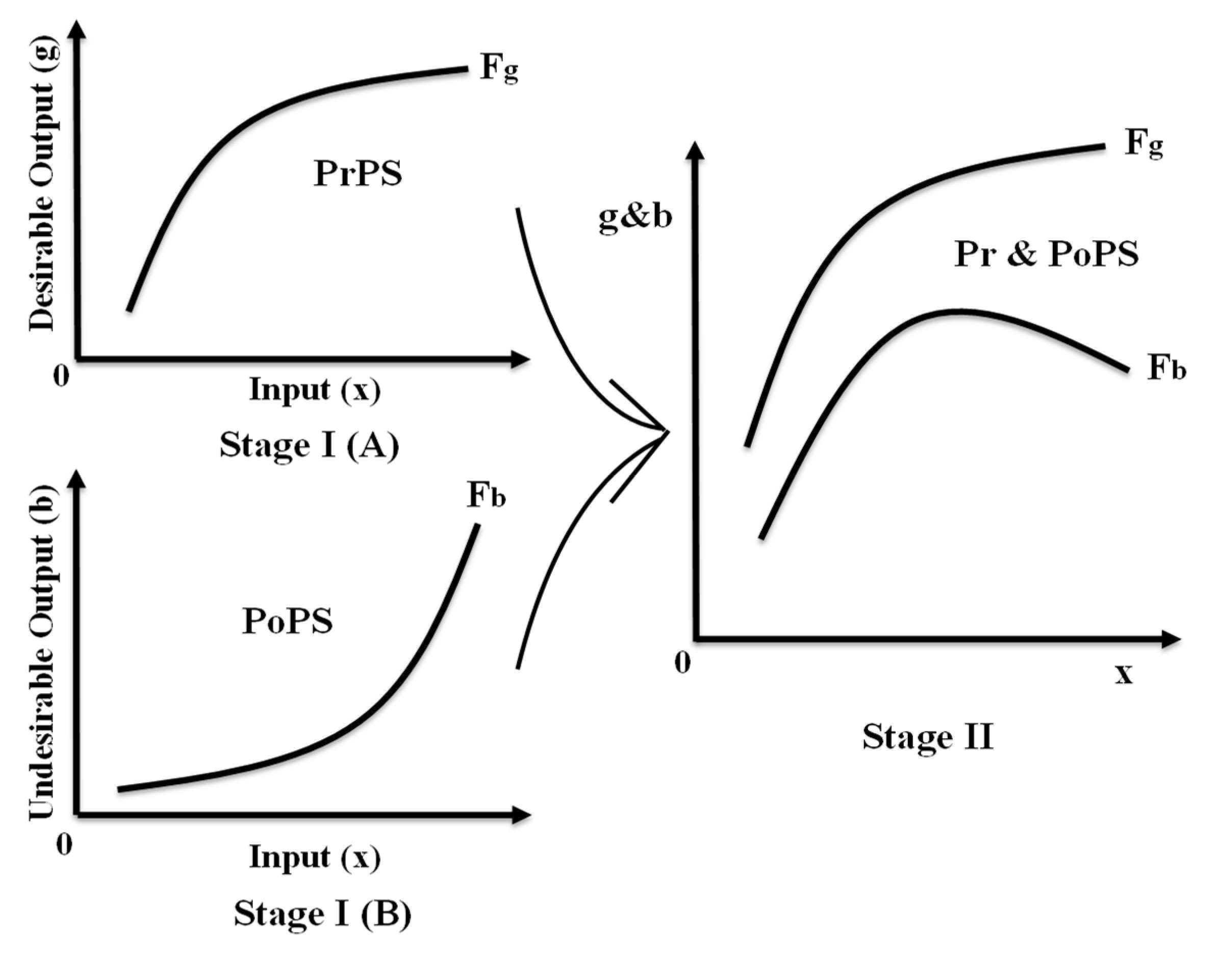
3.3. A Shape Change of Production and Pollution Functions
Figure 3 depicts a shape change of production and pollution functions under the assumption of the null-joint hypothesis. First stage (I) is separated into two sub-stages: (I-A) and (I-B). The sub-stage (A) of stage (I) indicates the production relationship between an input (
x) and a desirable output (
g) under the assumption that all DMUs produce a same amount of undesirable output (
b). For our visual description, we assume that production factors have a single component.
A Production Possibility Set (PrPS) depicts the efficiency frontier () in the x-g space. Stage (I) has the sub-stage (I-B). A Pollution Possibility Set (PoPS) is above the curve that represents the efficiency frontier () in the x-b space under the assumption that they produce the same amount of a desirable output (g). An important feature of stage (I-B) is that the production possibility set (I-A) is independent from the pollution possibility set of the stage.
To unify the two sets related to the first stage (I), we incorporate an assumption that “B is a by-product of G”. While seemingly trivial, the assumption significantly changes the structure of DEA environmental assessment. Specifically, the assumption leads the two efficiency frontiers (and ) to be shaped by two convex forms as in stage II. It is important to note that the frontier () should have an increasing trend along with an input increase. However, the frontier () should have an increase and decrease trend, because we are interested in reducing the volume of b. Both curves should be convex forms because of the assumption. The Production and Pollution Possibility Set (Pr&PoPS) locates between and. This study considers that DMUs in Pr&PoPS maintain their sustainability because they have feasibility in both production and pollution.
4. Methodology
This section discusses the computational framework of DEA models under natural and managerial disposability. Then, the two disposability concepts are reorganized under the null-joint relationship. In the DEA implementation, this study considers n DMUs (i.e., an entity to be examined). The subscript (j) indicates the j-th DMU (j = 1, ..., n), which uses m inputs to yield both s desirable and h undesirable outputs. The vector X indicates such input resources. The vectors G and B denote desirable and undesirable outputs, both of which show opposite directions for optimization. It is widely known that DEA does not assume any functional form to express the relationship among X, G and B. Their components are all strictly positive at the t-th period (t = 1, ..., T). Each DMU seeks to maximize its own economic and environmental efficiency measures, whose unified efficiency is relatively determined by comparing its performance with the others in single or multiple period(s).
Major variables used in DEA models are as follows: is the i-th input of the j-th DMU in the t-th period, is the r-th desirable output of the j-th DMU in the t-th period, is the f-th undesirable output of the j-th DMU in the t-th period,is an unknown weight of the j-th DMU at the p-th period and is a prescribed small number. Note that we introduce the small number to make multipliers (i.e., weights among components of X, G and B) strictly positive.
Following [
27], this study specifies the three sets of data ranges (
R) according to the upper and lower bounds of the three production factors as follows:
The range allocation is important in computing the efficiency of each DMU. That is, a difficulty of DEA applications is that “zero” occurs in their multipliers on X, G and B. The occurrence of zero clearly indicates that the corresponding factor is not fully utilized in the DEA-based efficiency computation. The result is unacceptable. The range allocation, as specified above, can avoid such a difficulty, even if most previous studies have neglected the occurrence of zero in DEA applications (and so are unreliable).
4.1. Formulation
It is necessary for DEA to reduce the influence of a “frontier crossover” among multiple periods by combining multiple periods into a cross-sectional one. For example, an efficiency frontier in the t-th period may retreat from the (t−1)-th period in a data space so that we cannot measure an efficiency difference between the two periods. To avoid this type of difficulty, the proposed approach incorporates multiple periods in which we combine multiple observations like cross-sectional data. No previous study has discussed the new data treatment, maybe because it maintains computational tractability.
4.1.1. Natural Disposability
We first formulate the model under the concept of natural disposability, which means that a DMU can reduce
X in order to decrease
B [
27]. This study uses the following radial model to measure the
UEN on the
k-th DMU at the
t-th period:
The objective function indicates the level of
UEN with a possible existence of UC (Undesirable Congestion); the conceptual implications are elaborated in [
26,
27]. The variable (
), implies an inefficiency measure, which is unrestricted (URS) in Model (1). This model is formulated by constant RTS because no restriction is allocated to
. Reference [
27] provides a detailed description on RTS.
The
UEN of the
k-th DMU in the
t-th period is measured by the following equation:
All unknown variables in Equation (2) are obtained from the optimality of Model (1). This study measures the SGN of the
k-th DMU in the
t-th period as follows:
The equation implies that the rate of SGN increases from the ( t– 1)-th to t-th period.
4.1.2. Managerial Disposability
The second model is for computing UEM. The concept of managerial disposability means that the DMUs, through managerial efforts, can increase
X to increase
G and simultaneously decrease
B [
27]. Following [
27], we obtain the model by reorganizing Model (1) by the following formulation:
The description of Model (1) is applicable to Model (4). An important feature of Model (4) is that it changes
in Model (1) to
in order to attain the status of managerial disposability. The model is organized under constant DTS [
27].
The UEM on the
k-th DMU in the
t-th period is measured by
All unknown variables in (5) are obtained from the optimality of Model (4). This study measures the SGM of the
k-th DMU in the
t-th period as follows:
The equation implies the rate of SGM increases from the (t – 1)-th to t-th period.
4.1.3. Null Joint Relationship
An important assumption to be considered in DEA applied to energy and environment is the null-joint relationship that “undesirable outputs are by-products of desirable outputs”. The hypothesis implies that
B does not exist without
G. The assumption makes it possible that we can unify Models (1) and (4). For example, we have the following combined formulation under natural disposability [
27]:
An important feature of Model (7) is that the
B related constraints are formulated by
. The analytical structure of
B is formulated like
G, because
B components are assumed to be the by-products of
G. A unified efficiency measure on the
k-th DMU is measured as follows:
All variables are obtained on the optimality of Model (7). This study measures the SGNM of the
k-th DMU in the
t-th period as follows:
The equation implies the rate of SGNM increase from the (t – 1)-th to t-th period.
4.2. Implications of Three Formulations
At the end of this section, we need to describe the unique structure of Models (1), (4) and (7). The left-hand sides of the three models contains all data sets from the first period to the t-th period (p = 1, ..., t). Meanwhile, the right-hand sides contain only the data set in the t-th period. We incorporate the data treatment to handle a possible occurrence of a frontier overlap among multiple periods. The treatment produces an efficiency frontier that covers DMUs in all periods. The t-th period may change from the first to the last (T) period. Therefore, the efficiency frontier moves along with the t-th periods.
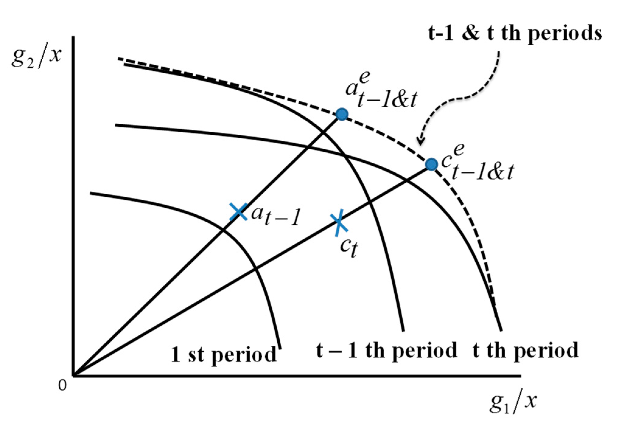
To visually describe the importance of such a time accumulation in DEA measurement, this study includes
Figure 4, which depicts a possible occurrence of the frontier crossover between the (
t−1)-th and
t-th periods. The horizontal axis indicates
g1/x and the vertical axis indicates
g2/x. The figure drops
b by assuming that
b is the same for all DMUs. The performance of DMUs in
Figure 4 is measured under the assumption of natural disposability. The figure shows that the efficiency frontier shifts between the two periods. As a result, it is necessary to combine the two frontiers to form a new efficiency frontier, which is indicated by the dotted curve in
Figure 4. The performance of DMU {a} is observed as
at−1 at the (
t−1)-th period, and DMU {c} is observed as
ct at the
t-th period. Both need to shift their locations to
and
on the newly shaped (dotted) efficiency frontier for the
t−1 and
t periods. The superscript (e) indicates an efficiency frontier. This type of crossover may occur between any periods from
p = 1 to
p = t. Therefore, Model (1) combines all periods in their left hand of the formulation.
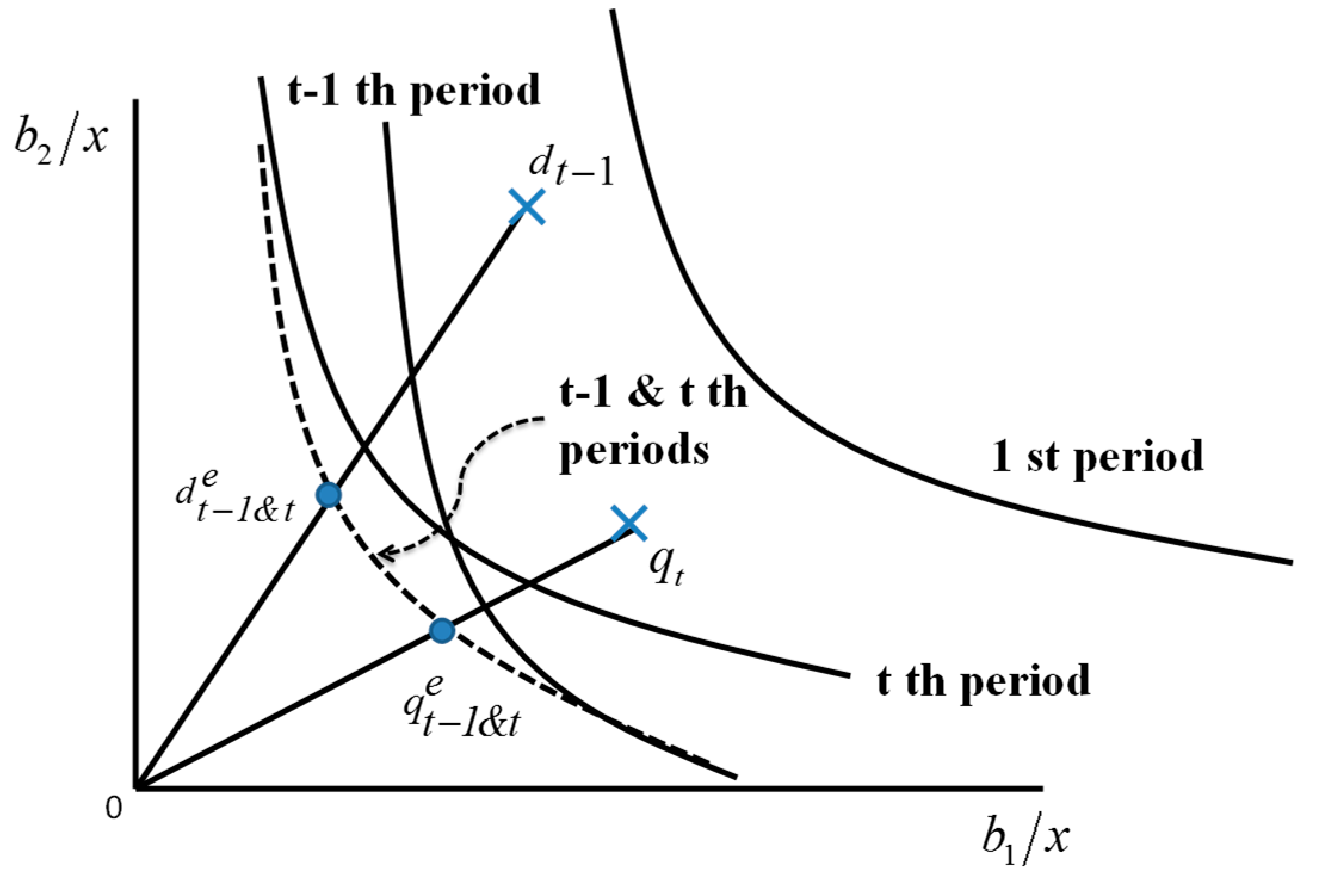
In a similar manner,
Figure 5 visually describes a frontier crossover between the
t−1 and
t-th periods under managerial disposability. The horizontal axis indicates
b1/x and the vertical axis indicates
b2/x. For our visual description, the figure drops
g from
Figure 5 by assuming that
g is same on all DMUs. The performance of DMUs in
Figure 5 is measured by managerial disposability. In the figure, an efficiency frontier retreats between the two periods. Hence, it is necessary to combine the two frontiers to shape a new efficiency frontier, or the dotted line in
Figure 5. The superscript (e) indicates an efficiency frontier. This type of crossover may occur between any periods from
p = 1 to
p = t. Therefore, Model (4) combines all periods in the left hand of the formulation.
At the end of this section, it is important to note two unique features regarding the proposed approach. One of the two is that it is different from previous efforts such as the “Malmquist index approach” [
28], which measures a frontier shift among multiple periods and “window analysis” [
29] that measure a shift of efficiency measures among multiple periods. The proposed three models do not measure the frontier shift as measured by Malmquist index approach. They do not measure an efficiency shift within limited adjacent periods (e.g.,
t = 3, 4, 5). Rather, they cover all periods. Such is the difference between the proposed models and the window analysis. Thus, our approach is different from the two previous approaches. The other unique feature is that the proposed approach belongs to the radial measurement. DEA environmental assessment is usually classified into three categories (radial [
30], non-radial [
31] and intermediate [
32]). As an extension of this study, we need to examine to examine whether any methodological bias (i.e., different methods produce different results) occurs in the data set used in this research. This is an important future task.
5. Data and Variables
This study builds the data sample mainly from the China Statistical Yearbook and China Energy Statistical Yearbook. These two yearbooks are published annually by the National Bureau of Statistics of China. Since the country’s yearbooks have missing data entries, we occasionally resort to the provincial yearbooks as a complementary source of data. The basic sample covers 31 provincial-level administrative divisions of China and the annual periods for 2004–2017 (Of the 34 provincial-level administrative divisions in China, Hong Kong, Macau and Taiwan are excluded from the sample due to lack of data).
We employ the following input variables in assessing sustainable development by the DEA. There are three inputs: (a) labor, (b) capital stock and (c) energy use. Labor represents the number of persons employed in a province and is measured in millions. Capital stock of a province is computed by the perpetual inventory approach [
33] and measured in billion RMB. Energy use of a province is measured by thousand TCE.
Using the three inputs, each province produces one desirable output and three undesirable outputs. The desirable output, GDP, is measured in billion RMB. The undesirable outputs include (a) wastewater, measured in million tons, (b) SO
2, measured in tons, and (c) CO
2, measured in million tons. Note that the China Statistical Yearbook also reports emissions of other pollutants such as NO
x, PM2.5 and PM10. However, the collection of such data only starts in very recent years and we have to exclude them from this study in order to maintain a reasonable duration of data. Climate change is at the forefront of the environmental policy of China, as the country is becoming a global climate leader. CO
2 emissions should therefore be taken into account. However, the Yearbook does not report provincial-level CO
2 emissions. We obtained provincial CO
2 emissions data from China Emission Accounts and Datasets (CEAD). CEAD, funded by some high-profile institutions such as Chinese Academy of Sciences and the National Natural Science Foundation of China, is a research program that measures provincial and sectoral carbon emissions of China. However, CEAD only provides data up to 2015 and does not include Tibet in the sample [
34]. Accordingly, we will run separate models for 30 provinces over 2004–2015 in order to incorporate the effects of climate change.
Table 1 reports the descriptive statistics for years 2017 and 2004 respectively. We observe that labor, capital stock, energy use and GDP have increased from 2004 to 2017. For the three pollutants, the SO
2 emissions have greatly decreased, while wastewater discharge and CO
2 emissions have dramatically increased.
6. Empirical Results
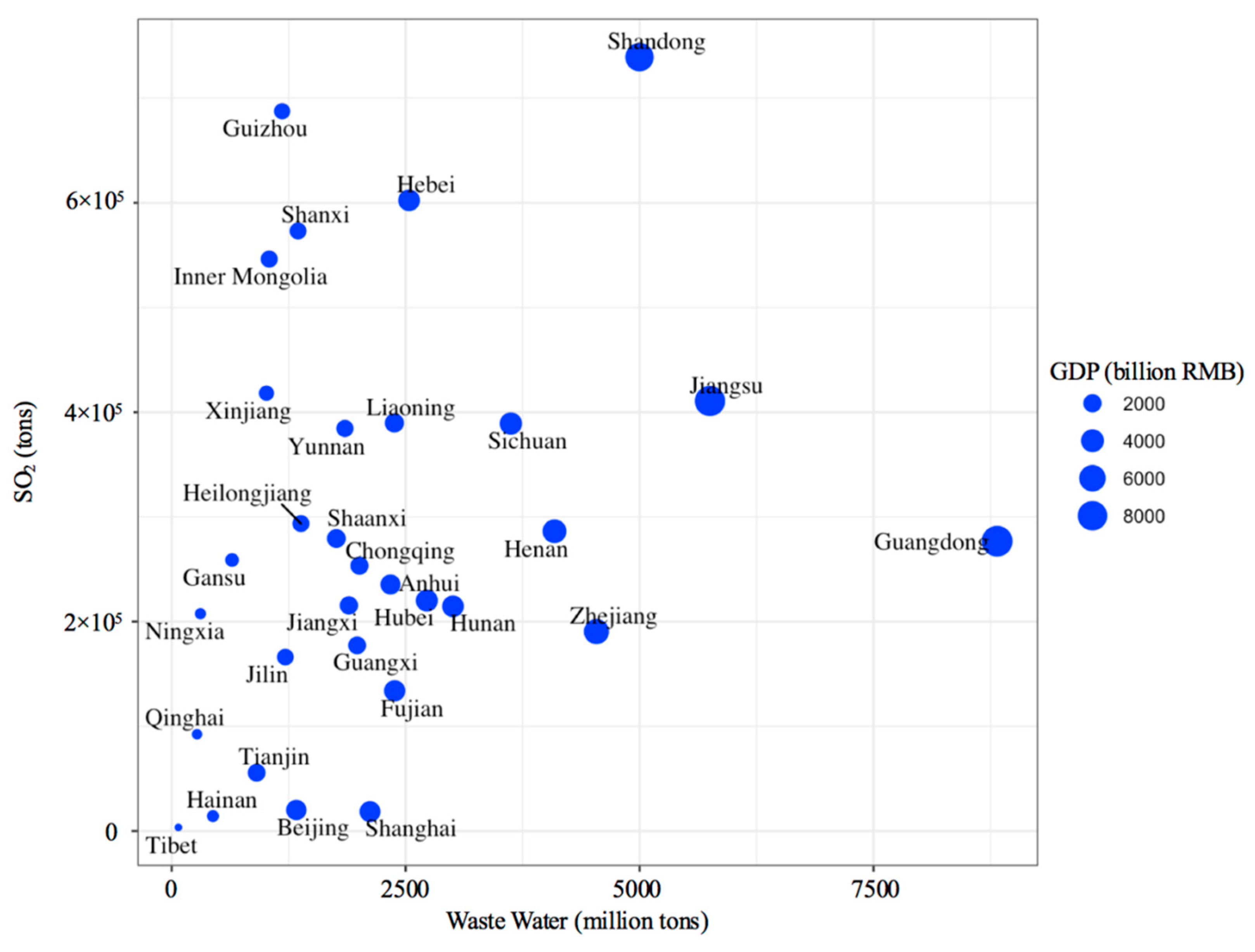
To illustrate the up-to-date provincial economy and pollution,
Figure 6 shows the GDP, SO
2 and wastewater for each province in 2017. We observe that the provinces exhibit a diverse pattern in economic and environmental performance. In general, economic diversity can be traced back to the economic structure. Different provinces have different economic structures and different economic development models. For instance, Beijing and Shanghai, with their economy concentrated on the service sector, produce low pollution relative to their GDP. Hebei, Guizhou, Shanxi, and Inner Mongolia have high levels of SO
2 emissions relative to the sizes of their GDP, due to the significant shares of mining and metal industries in their economies. Guangdong has significantly higher wastewater discharge than any other provinces, even though a few provinces have comparable GDP. This is because Guangdong, as the growth engine of China’s economy, has a strong manufacturing sector, especially in industries consuming large quantities of water such as electronics, textiles, and pulp and paper. Shandong has the highest SO
2 emissions, to a large degree because the province has the highest electricity generation from coal-fired power plants in the provinces (according to a report by the National Bureau of Statistics). Tibet has the lowest SO
2 emissions and wastewater discharge, as well as the smallest economy among the provinces. This is because Tibet’s unique plateau environment cannot support many large factories and manufacturing industries. Hainan follows Tibet in the second place in SO
2 emissions, since a significant part of its economy is made up by tourism rather than manufacturing. Overall, the diverse provincial-level economic and environmental performance shown in
Figure 6 prods us to ask how to quantify the sustainable development by a single index.
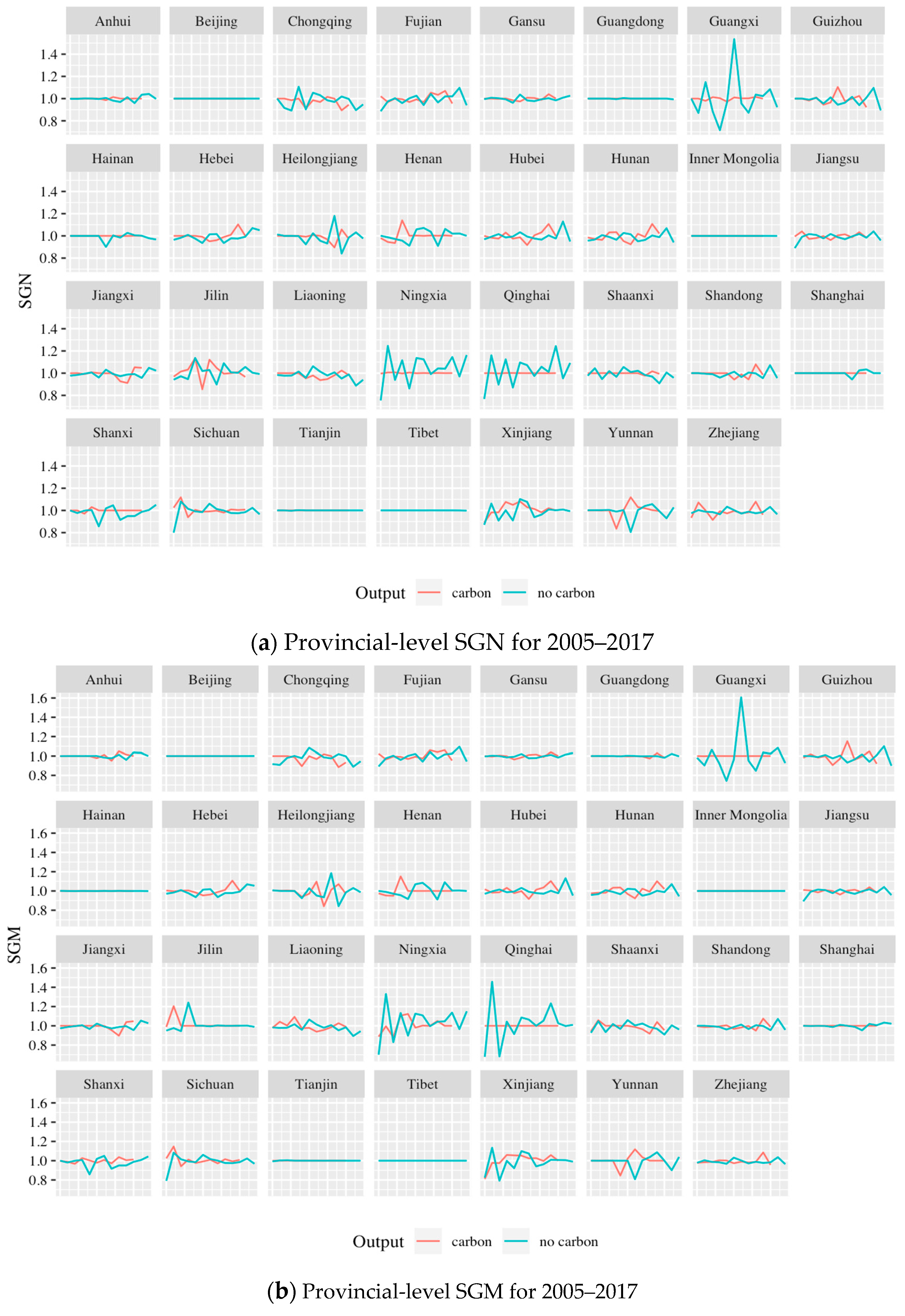
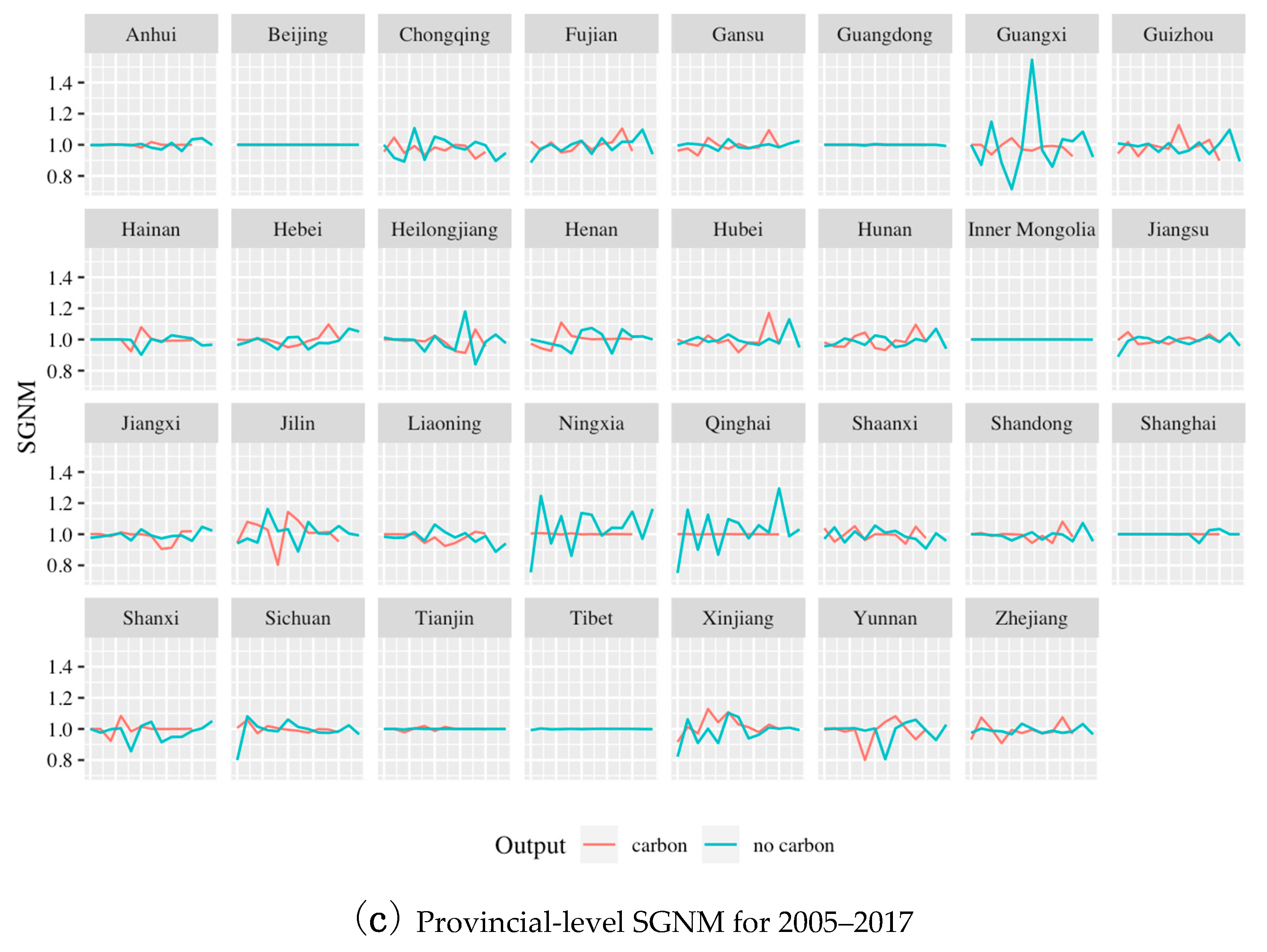
Next, we numerically solve Models (1)–(9) based on the data sample and analyze the results. The provincial-level SGN, SGM and SGNM over time are plotted in
Figure 7. To get a glimpse of the computational results,
Table 2 further reports the SGN, SGM and SGNM for 2017. Note that the first year with indices available is 2005 rather than 2004, since the indices are ratios of DEA scores in two consecutive years. From
Figure 7, we observe that some provinces have very stable performance while there are a few provinces displaying dramatic changes in the sustainability indices over time.
For example, Anhui, Beijing, Gansu, Guangdong, Inner Mongolia, Sichuan and Tianjin have SGN, SGM and SGNM values consistently close to unity in every single year. This means that, no matter what the criteria are, these provinces have been maintaining very stable sustainability performance relative to other provinces. When CO
2 is excluded from the outputs, Ningxia, Xinjiang and Yunnan are obviously the provinces with the largest swings in all three indices. For instance, for Ningxia, the highest SGM is above 1.3, whereas the smallest SGM is below 0.8. The large variations of sustainability indices can be attributed to their economic structure. All three provinces have a relatively simple economic structure and rely heavily on the agriculture and tourism industries for economic growth. The performance of the agriculture industry and that of the tourism industry are subject to natural conditions and tend to display a high degree of volatility. Therefore, it will cause fluctuations in the economic sustainability index of these provinces. For instance, the quarterly GDP growth rate of Ningxia can be as high as 19.0% in 2010 and as low as 6.9% in 2014 and 2016 (according to Ningxia’s official quarterly GDP data). In addition, some provinces show stable performance in a certain period but are volatile at other times. For instance, Hainan and Henan are quite stable in the first half of the horizon but are volatile in the second half. This may be due to changes in the economic structure of the province. Further, we note that in
Figure 7 and
Table 2, the three indices are close to each other. Therefore, the results are quite robust regardless of which method is used. If CO
2 is included as part of the outputs, the result can be drastically different for certain provinces. For example, SGN, SGM and SGNM of Qinghai are at 1.0 if CO
2 is included, but they swing a lot if CO
2 is excluded.
Table 3 documents the provincial-level geometric means and ranks of SGN, SGM and SGNM during 2005–2017 without CO
2 in outputs and 2004–2015 with CO
2. The geometric means represent the overall sustainable development for the annual periods under study. They can also be interpreted as the annual sustainability growth rates on average. Without CO
2, the province with the best overall sustainability growth for 2004–2017 is Ningxia, in all three indices (SGN = 1.032, SGM = 1.023, SGNM = 1.032). If CO
2 is included, Ningxia is no longer the best province but still maintains a reasonably good performance, with ranking at the 5th, 19th and 3rd positions for the three indexes. This is surprising, since Ningxia, situated in the northwest inland of China, is generally regarded as a less developed province with a reasonable but not stellar growth rate. However, taking environmental factors into account, the results indicate that Ningxia has been able to achieve the greatest improvement in sustainability enhancement. This implies that the province has achieved exceptionally well in coordinating economic growth and environmental protection. Another notable province is Jilin, which is consistently ranked as a top-three province in all indexes with and without CO
2. With regard to the underperformers, the province of Chongqing notably has the worst performance among the provinces in almost all indexes with and without CO
2. On the other hand, Chongqing has stellar double-digit GDP growth rates in 2010s, and is generally regarded as the fastest-growing economy among the all the provinces in China. The economic growth of Chongqing is fueled by infrastructure investment and urbanization. The contrast between the province’s fast economic growth and the sustainable development raises the issue that Chongqing has not been able to balance economic development and environmental protection in an appropriate way. A few provinces’ performance depends critically on whether CO
2 is included. With CO
2, Xinjiang is close to bottom, while without CO
2 the province becomes a top performer. This is determined by its unique environmental and geographical factors. Hence, CO
2 plays an important role in determining the province’s performance relative to others.
Table 3 also demonstrates that the majority of the provinces have similar ranks in terms of all three indices. The several exceptions with rank differences larger than five are Guangxi, Hainan, Henan, Qinghai and Shaanxi. Guangxi, Hainan, and Henan have better ranks in SGM than SGN and SGNM, and the ranks of Qinghai and Shaanxi in SGM are worse than SGN and SGNM. Ranking higher in SGM than SGN and SGNM implies that Guangxi, Hainan and Henan have done well in taking managerial efforts to control pollutions. Qinghai and Guangxi are not doing very well in adopting management measures to control pollution. Specifically, through managerial efforts, they have increased the inputs to increase the desirable outputs and simultaneously decrease the undesirable outputs. Ranking lower in SGM implies Qinghai and Shaanxi should improve their managerial practices.
Table 4 reports the annual means of SGN, SGM and SGNM for 2005–2017. During this 13-year period, without CO
2 being included, for roughly half of the years, the sustainability indices are greater than unity. After CO
2 is included, the three indexes exhibit similar patterns as without CO
2, except for a few data points. For example, in year 2010, with CO
2 the values of SGN and SGM are less than one, but without CO
2 they are greater than one. The difference indicates that CO
2 is a factor that drags down the overall performance in 2010.
7. Conclusions and Policy Implications
This study investigated the provincial-level sustainable development of China for the period 2004–2017. Three indices, measuring sustainable development under natural disposability, managerial disposability and null-joint relationship, were developed and computed by DEA. The assessment considered capital stock, labor, energy use, GDP, SO2 emissions, wastewater discharge and CO2 emissions. In previous studies, few considered the use of wastewater as an indicator for China’s sustainable development research. We find that due to the unique environmental, geographical and economic factors of each province, there are various sustainable development patterns. During the time horizon under study, a smaller set of provinces were able to maintain very stable sustainable development from year to year and a few others displayed quite dramatic changes in sustainability. In addition, the fast-growing economies of some provinces contrast sharply with poor sustainable development. They failed to deal with the economic development and environmental protection in a balanced way. Moreover, some provinces showed significant differences in the comparison of sustainable development with and without CO2.
The aforementioned results bear the following implications for provincial administrators and national policymakers. First, the diverse pattern of provincial-level sustainable development observed in 2004–2017 implies that a one-size-fits-all environmental policy made by the central government is not likely to be the best solution. Traditionally, China has been a country where local policies are mostly dictated and closely enforced by the central government. While this one-size-fits-all governance model is desirable in certain scenarios, it may not generate the best result in sustainability. The central government has realized the problem and adopted more flexible policy frameworks to accommodate the different situations and needs of the provinces. For instance, the newly founded Ministry of Ecology and Environment has clearly indicated that policymaking should account for regional differences and a uniform forced shutdown policy should be avoided [
35]. Second, for provinces with large variations in the three sustainability indices, provincial policymakers should strive to ensure more consistent performance by imposing more consistent management practices, so the provinces can act in a more synchronized way. While there is a solid consensus that environmental protection is an important problem that should be dealt with, what specific actions should be taken remains a highly contentious issue. Sometimes the provincial policy can be short-lived and precarious. Policymakers may consider providing guidelines or even regulations to govern the local authorities to achieve stable performance. Finally, the government must avoid a development model that depends on consuming resources to improve the economy. Lucid waters and Lush Mountain are invaluable assets. The government should promote green, circular and low-carbon development and strive to build national ecological security.
The study has the following two limitations. First, although the horizon under study in this paper is longer than existing studies on provincial-level sustainability of China to the best of our knowledge, it covers only one third of the 40 years that have passed since the “reform and opening-up” of China. Thus, the analysis can only generate a partial view, and it is hard to evaluate the long-term effect of the reforms on sustainability. Second, the DEA method itself cannot provide statistical inference, so it has to be combined with other methods to test the statistical significance of the empirical results.
This study suggests avenues for future research. First, due to lack of data, in this paper we were unable to include some important air pollutants such as NO
x, PM2.5 and PM10. Since the National Bureau of Statistics of China has started to collect and report data on those pollutants, with sufficient data in the future we will be able to assess sustainability in a more comprehensive way [
3]. Second, it would be interesting to explore the driving forces behind sustainable development in more detail. We briefly touch on the issue in this article, but more rigorous analysis and conclusive evidence are necessary for pinpointing the determinant factors. Finally, it is hoped that this study makes a contribution to DEA-based environmental assessment. We look forward to seeing future extensions as suggested in this research.


