Productivity-Index Behavior for a Horizontal Well Intercepted by Multiple Finite-Conductivity Fractures Considering Nonlinear Flow Mechanisms under Steady-State Condition

Abstract

In this paper, a mathematical model is proposed to investigate the effect of nonlinear flow mechanisms on productivity-index (PI) behavior in hydraulically fractured reservoirs during steady-state condition. This approach focuses on the fact that PI approaches a constant value at a certain time, indicating the beginning of steady state. In this model, the reservoirs are considered as an elliptical-shaped drainage with constant-pressure boundary, which is depleted by a multiple-fractured horizontal well (MFHW), and various nonlinear flow mechanisms, such as the non-Darcy flow effect and pressure-dependency effect, control flow patterns in the hydraulic fractures. Then, an exact algorithm of solving the resulting nonlinear equations is developed to obtain the PI of MFHW using a semi-analytical approach. Next, type curves are generated to investigate the influences of flow mechanisms and fracture properties on PI. The most interesting points in this study are the following: (1) PI is determined by the properties of MHFW (i.e., dimensions and configuration), the reservoir geometry, and flow mechanism; (2) PI is deteriorated by non-Darcy flow caused by inertial forces; and (3) PI is reduced under the influence of pressure sensitivity caused by the degradation of dynamic conductivity. Generally, this study provides a significant insight into understanding the factors affecting the productivity of a MFHW with nonlinear flow mechanisms.

1. Introduction

With the success of Bakken tight oil resource in the United States, tight oil and gas reservoirs have become a significant source of hydrocarbon supply globally [1]. Subsequently, the technology of horizontal drilling combined with hydraulically fracturing has effectively enabled commercial production from the reservoir with extremely low permeability [2,3]. In practice, the characteristics for a stimulated well are identified by flow regimes; for example, the approach of pressure-derivative is used to identify flow-regimes for pressure transient analysis. For a multi-fractured horizontal well, the sequence of flow-regimes may be more complex (Figure 1) [4]. At some point after compound linear flow caused by the fracture interference, a compound elliptical flow regime (regime 5 in Figure 1a) would appear as the transient pressure waves move past the ends of the fractures [5,6]. Put another way, the compound elliptical response is the pseudo-steady state in an infinite drainage area. It is noted that the isopotential line approximates to an elongated elliptical shape for a long horizontal wellbore, as shown in Figure 1b.

In physics, the performance of a fractured reservoir is determined by numerous factors such as formation petrophysical properties, fluid properties, and reservoir and wellbore configuration [7]. Numerous methods are provided to capture the physics of fluid flowing in the fractured reservoirs. Originating from the pioneer work suggested by Warren and Root [8], the fractures are represented by a 3D uniformly spaced fracture network, and the matrix blocks are contributing sources. It is a fictitious homogeneous porous medium. As a result, multiple-continuum models are used to compute the transient response of uniform naturally (continuously) fractured reservoirs. In analytical modeling, these models consist of a set of one-dimensional linear flow regions, and the main difference is the way in which these regions are coupled [9,10,11]. Therefore, it is difficult for the multiple-continuum model to capture the intrinsic behavior of complexity of nonuniform naturally fractured reservoirs, such as hydraulically fractured reservoirs. To capture the strong heterogeneity between fracture and matrix, various improved techniques are presented to subdivise the grids, such as the embedded discrete fracture model (EDFM), Galerkin finite-element method (FEM), and discrete-element method (DEM) [12,13,14]. However, it is still a huge challenge to obtain accurate transmissibility by computing the irregular connections between fracture segments. Considering the high computational burden and the great difficulties in gridding, the mesh-free semi-analytical method is necessarily developed as an alternative to the numerical simulation method. On the basis of the works suggested by Cinco-Ley et al. [15], various semi-analytical models, which have the flexibility of accounting for the individual fracture properties, are proposed to investigate the influence factors on the performance of the fractured reservoirs [16,17,18,19]. It is proven that the semi-analytical methods have huge potential in analyzing transient performance response and evaluating productivity of wells.

From the viewpoint of petroleum engineering, the effects of these parameters on reservoir performance can be represented by the productivity index (PI). It is defined as the ratio of production rate to a certain pressure drop. PI is determined by the flow regime, with different behavior characteristics with time. It starts out with a high value at an early time when the transient response is dominant. PI declines with time to a small value, and approximates to a constant value, known as stabilized PI, at a late time period when the compound elliptical response is reached [20]. Currently, most studies have put the focus on the transient productivity index to identify the flow regimes [21,22,23]. However, they found that the designed fractured wells do not usually result in the expected performance, which is attributed to the existence of nonlinear flows. From the viewpoint of multi-physics, the flowing in the underground porous media is the result of fluid–thermal–solid coupling [24]. The reservoir production is generally regarded as the isothermal process; therefore, the thermal is not considered in the production simulation. Strictly speaking, the rock deformation may have a significant effect on fluid flow owing to fluid-particle interactions. According to the conclusions presented by Zhang and Tahmasebi [25,26], the effect of solid deformation on fluid flow, especially in hydraulic fractures, could be incorporated by regarding the porosity and permeability as a function of stress changes. In other words, the conductivity of hydraulic fracture changes because of a variety of mechanisms, including fracture closure under high effective stress and permeability loss as a result of proppant embedment and crushing. Besides, non-Darcy flow may occur in the fracture when the well is produced at a high flow rate [27]. Therefore, the nonlinear flow effects have to be taken into account to investigate the effect of nonlinear behaviors on the performance of a vertical well and fractured well in the infinite-acting reservoir. Limited efforts have been made to examine the effects of non-Darcy flow and pressure-sensitive conductivity on the performance of horizontal wells with multiple fractures. Wu et al. [28] used a numerical approach to investigate the non-Darcy effect in an unconventional gas reservoir. Lin and Zhu [29] developed a slab source method to evaluate the performance of horizontal wells with or without fractures using an analytical approach. Besides the non-Darcy effect, pressure sensitivity in the fracture may also exert an important influence on the transient response. A transient pressure analysis for a vertical well intercepting a dynamic-conductivity fracture has been conducted using analytical and numerical methods. Pedroso and Correa [30] developed a new model to investigate the effects of pressure-sensitive permeability on the flow behavior of a fractured well. Zhang et al. [31] presented the results of a study that analyzed the build-up of pressure in a vertically fractured well with a stress-sensitive conductivity in the fracture. Yao et al. [32] studies the effect of dynamic conductivity on the transient performance of multiple fractured horizontal well.

To the best of our knowledge, few papers are published to study the productivity index of a multiple-fractured horizontal well (MFHW) in a finite drainage area with an elliptical boundary under nonlinear flow conditions. The objective of this work is to quantify the effect of non-Darcy flow and pressure sensitivity on the inflow performance of a MFHW. First, we establish a hybrid model that describes Darcy flow in the reservoirs toward hydraulic fractures, as well as non-Darcy flow along the fracture with pressure-dependent conductivity under steady-state conditions. First, a mathematical model is established to describe the fluid flow depleted by a MFHW in a reservoir with elliptical-shaped boundary, with the flexibility of accounting for fracture properties (i.e., fracture dimensions and configuration). Next, nonlinear flow mechanisms in the fracture, including stress-sensitivity effect and non-Darcy flow condition, are taken into account, which results in the nonlinearity in partial differential equation. Then, the technique of dimension transformation is used to render the resulting nonlinear equations amenable to linear treatment, and an effective and efficient algorithm is developed to solve the model. Finally, a study for sensitivity analysis is introduced to investigate the effect of fracture properties and nonlinear flow mechanisms on the productivity-index behavior.

2. Model Assumption

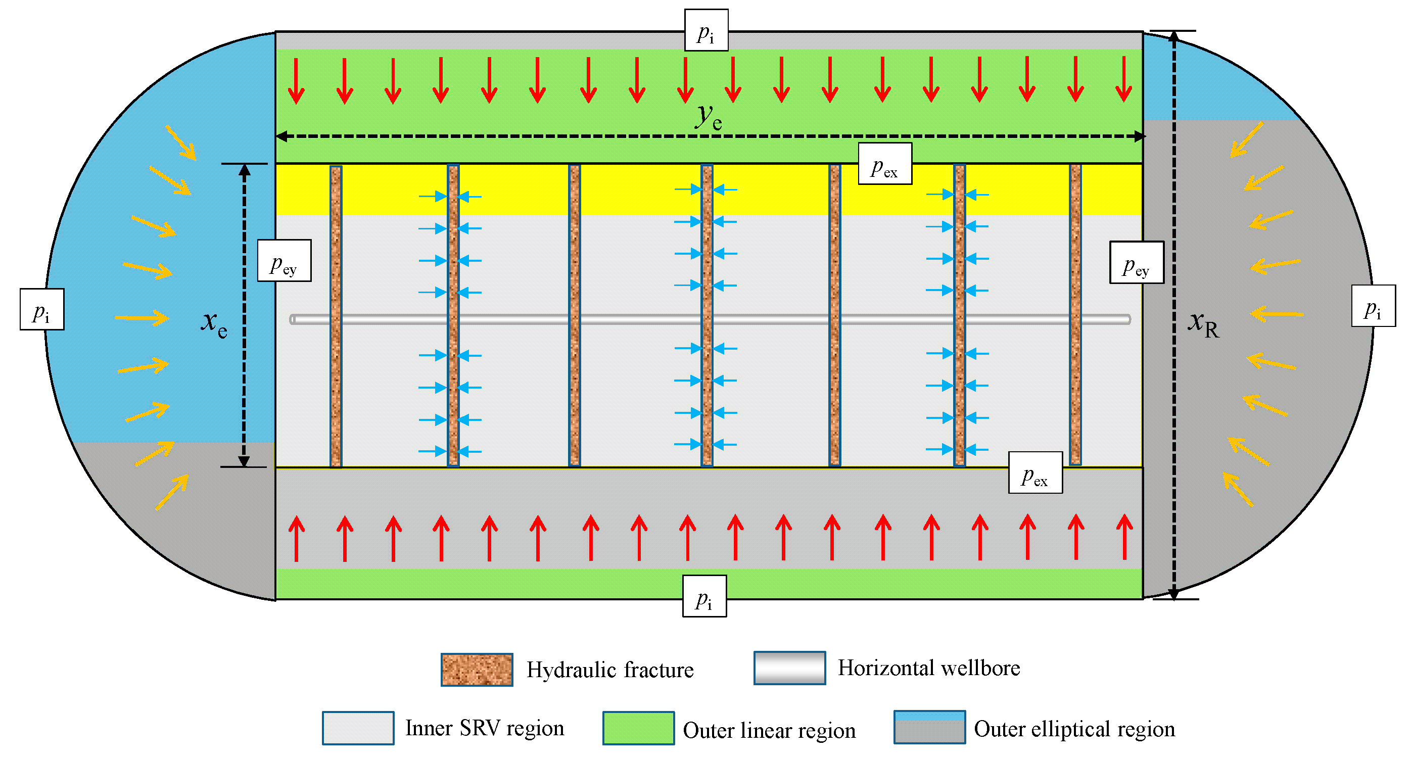
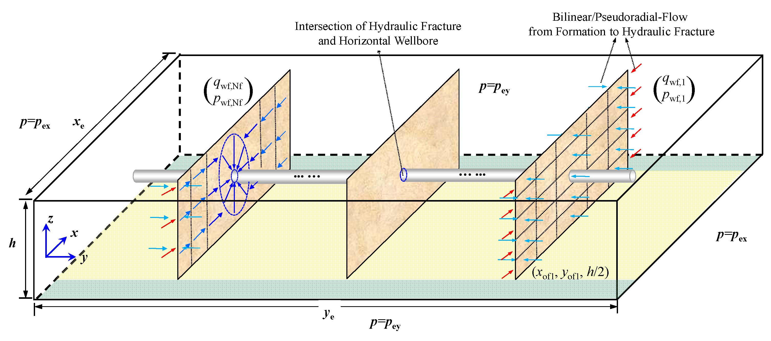
2.1. Physical Model

In this physical model, a horizontal well is located in the center of a homogeneous reservoir with an elongated elliptical boundary. The whole drainage area consists of several different flow patterns in four contiguous flow regions, as sketched in Figure 2, including (1) the hydraulic fractures, (2) the inner stimulated rock volume (SRV) region impacted by hydraulic fracturing, (3) the outer linear region beyond the extent of the SRV, and (4) the outer elliptical region beyond the tips of the horizontal wellbore.

Different from the anisotropic characteristics in a naturally fractured reservoir, where a large number of nature fractures are uniformly and globally distributed [33,34,35], this paper assumes that the reservoir is stimulated by several hydraulic fractures, so the resulting hydraulically fractured reservoir is regarded as isotropic. In addition, there are some necessary assumptions, as follows:

• The reservoir is horizontal and of uniform thickness, with impermeable lower and upper boundaries. The pressure on the outer boundary in the x–y plane keeps constant.
• Along the horizontal wellbore, multiple hydraulic fractures are evenly distributed. Hydraulic fractures are considered to be a finite conductivity.
• The wellbore is produced under constant-rate condition.
• Flow in the reservoir is assumed to be single-phase fluid (i.e., pure gas) with slight compressibility and constant viscosity.
• Fluid flowing in the fracture is assumed to be nonlinear.
• Fluids from the reservoir enter the wellbore only through hydraulic fractures, and the pressure loss in the wellbore is neglected.

2.2. Variables Definitions

To introduce the mathematical model conveniently and concisely, the dimensionless variables are defined, respectively, by

$$p_D=\frac{2\pi k_{m}h(p_i-p)}{q\mu B},{\xi }_D=\frac{\xi }{L_{ref}},q_D=\frac{q}{q_{ref}},C_{fD}=\frac{k_f{w}_f}{k_m{L}_{ref}}$$

(1)

When the flow in the fracture satisfies non-Darcy effect owing to high velocity, the corresponding dimensionless variables are defined as

$${(q_{DND})}_f=\frac{k_f\beta \rho }{\mu w_{f}h}{q}_{ref},\mathrm{and}{q}_{cD}=\frac{q_c}{q_{ref}},$$

(2)

When the fracture conductivity behaves pressure sensitivity, the corresponding dimensionless variables are defined as

$${\gamma }_{fD}=\frac{q\mu B}{2\pi k_{m}h}{\gamma }_f$$

(3)

where p_m is the pressure in the reservoir, Pa; p_f is the pressure in the fracture, Pa; p_i is the pressure on the elliptical boundary, Pa; p_ex is the pressure on the width of inner SRV region, Pa; p_ey is the pressure on the length of inner SRV region, Pa; (x_ofm, y_ofm) is the location of m-th fracture tip, m; x_e is the width of inner SRV region, m; y_e is the length of inner SRV region, m; x_R is the width of the whole drainage region, m³; h is the reservoir thickness, m; w_f is the fracture width, m; L_f is the fracture length, m; r_w is the radius of wellbore, m; L_ref is the reference length, m; q_fm is the function of inflow distribution along the m-th fracture, m²/s; q_wm is the production rate, m³/s; q_c is the influx rate, m³/s; μ is the viscosity, Pa s; B is the volume factor; γ_f is the permeability modulus, Pa⁻¹; and β is the Beta factor, m⁻¹. Here, the subscript D represents dimensionless variables.

3. Mathematical Model

3.1. Fluid Flow in the Inner SRV Region

The SRV region is regarded as a rectangular reservoir with constant-pressure boundary containing a set of hydraulic fractures, as shown in Figure 3. The diffusion equation governing fluid flow is given as the following dimensionless form:

$$\frac{{\partial }^2{p}_{mD}}{\partial x_D^2}+\frac{{\partial }^2{p}_{mD}}{\partial y_D^2}+2\pi {\displaystyle \sum _{m=1}^{N_f}{\displaystyle {\int }_0^{L_{fDm}}{q}_{fDm}(u_D)\delta (x_D-x_{ofDm}-u_D)\delta (y_D-y_{ofDm})d{u}_D}}=0$$

(4)

The outer boundary conditions are satisfied by

$$\{\begin{array}{l}{p}_{mD}(x_D=x_{eD},y_D)=p_{mD}(x_D=0,y_D)=p_{eDx}\\ p_{mD}(x_D,y_D=0)=p_{mD}(x_D,y_D=y_{eD})=p_{eDy}\end{array}$$

(5)

where there are N_f fractures in the SRV region, the dimensionless length of m-th fracture is L_fDm, and the dimensionless coordinate of m-th fracture tip is (x_ofDm, y_ofDm). The pressure on the outer boundary parallel to the fracture is p_eDx, and the pressure on the outer boundary perpendicular to the fracture is p_eDy.

Using Fourier transformation and inverse transformation (Appendix A), the dimensionless pressure distribution caused by N_f fracture is given by

$$p_{mD}(x_D,y_D)=p_{eDx}IB(x_D,y_D)+p_{eDy}ID(x_D,y_D)+2{\displaystyle \sum _{m=1}^{N_f}{\displaystyle {\int }_0^{L_{fDm}}{q}_{fDm}(u_D)\delta p_{uD}(x_D,y_D,u_D)d{u}_D}}$$

(6)

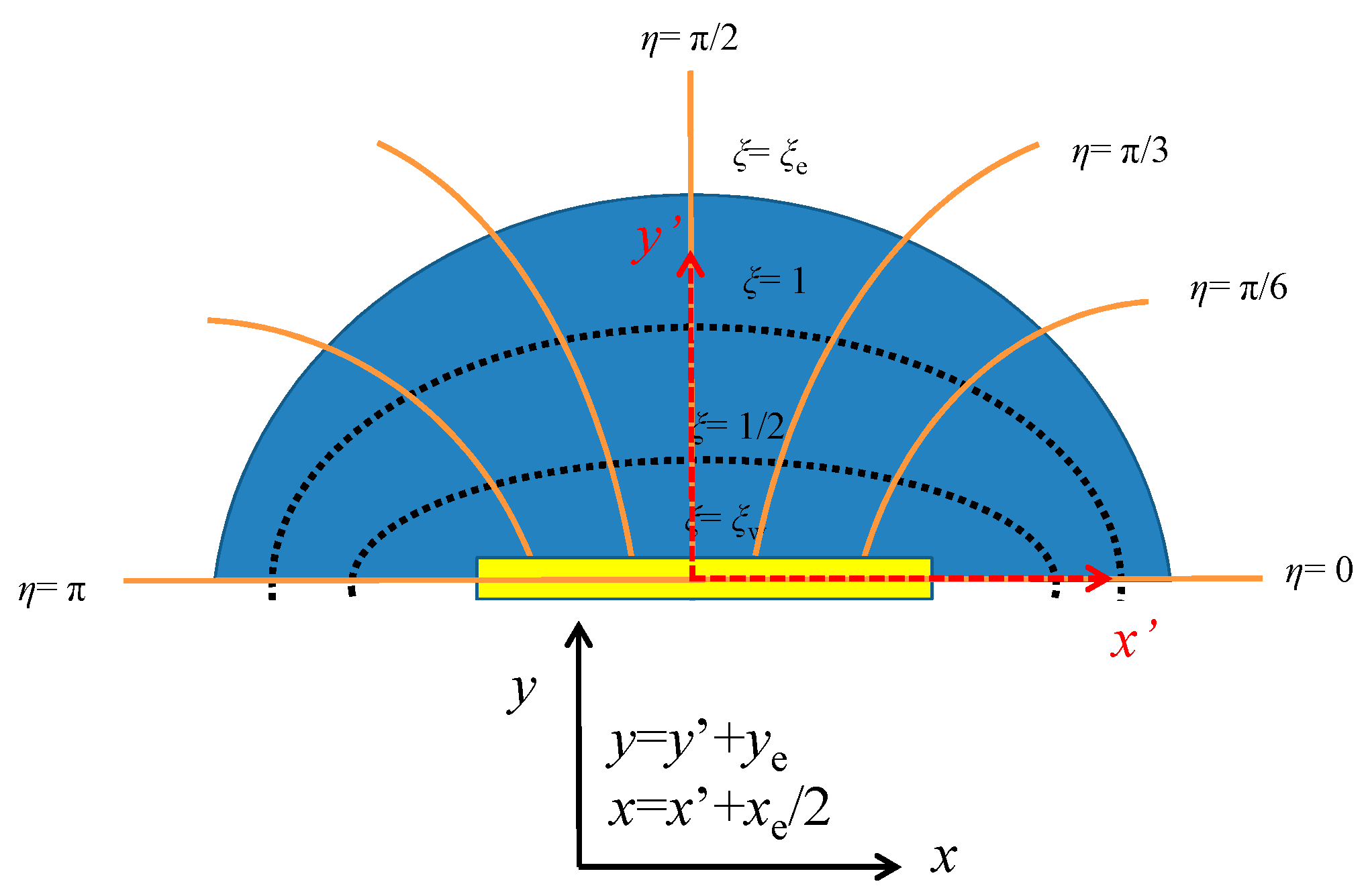
3.2. Fluid Flow in the Outer Region

The fluids stored in the outer region are depleted and then flow into the inner SRV region through the interface (denoted by the yellow block in Figure 4). The streamlines satisfy the hyperbolic shape (orange solid line in Figure 4), which are the counterpart of elliptical-shaped isopotential line (black dashed line). Once the fluids enter the inner region, the streamlines are in a linear shape around the interface. Therefore, the coordinate systems are divided into two subsets: 1D elliptical coordinate in the outer region (blue region), and 1D linear coordinate (yellow region).

The outer boundary satisfies the constant pressure of p_eD.

In the outer elliptic region, as shown in Figure 4, there are two sets of coordinates: the Cartesian coordinates (x’,y’) and the elliptic coordinates (ξ,η). The relationship is given by

$$x^{\prime }=(x_e/2)\cosh \xi \cos \eta ,y^{\prime }=(x_e/2)\sinh \xi \sin \eta$$

(7)

We used the elliptic coordinates to simulate the flowing process. The outer and inner boundaries of the elliptic region, represented by ξ in the elliptic coordinates, could be expressed using spatial variables in the Cartesian coordinates:

$$\{\begin{array}{l}{\xi }_e=\xi (x^{\prime }=x_R/2,y^{\prime }=0)=\ln [(x_R+\sqrt{x_R^2-x_e^2})/x_e]\\ {\xi }_w=\xi (x^{\prime }=0,y^{\prime }=0)=\ln 1=0\end{array}$$

(8)

The corresponding pressure gradient is written as the following dimensionless expression,

$${\left(\frac{\partial p_{mD}}{\partial {\xi }_D}\right)}_{{\xi }_D=0}=\frac{p_i-p_{ey}}{{\xi }_e-{\xi }_w}=-\frac{p_{eyD}}{\ln [(x_{RD}+\sqrt{x_{RD}^2-x_{eD}^2})/x_{eD}]}$$

(9)

Note that the flux inflow in Equation (9) is continuous on the interface between the outer elliptical region and inner SRV region. Meanwhile, the flowing is modeled using linear coordinates. As a result, the continuous condition is written in the form of the average integral, which is given by

$$\underset{ellipticflow}{\underbrace{\frac{1}{x_{eD}}{\displaystyle {\int }_0^{\pi }{\frac{\partial p_{mD}}{\partial {\xi }_D}|}_{{\xi }_D=0}d{\eta }_D}}}=\underset{linearflow}{\underbrace{\frac{1}{x_{eD}}{\displaystyle {\int }_0^{x_{eD}}{\frac{\partial p_{mD}}{\partial y_D}|}_{y_D=y_{eD}}d{x}_D}}}$$

(10)

It could be expressed as the function of p_eDx and p_eDy (Appendix B), which is written as follows:

$$A_2{p}_{eDx}+B_2{p}_{eyD}={\displaystyle \sum _{m=1}^{N_f}{q}_{wDm}{C}_{2,m}}$$

(11)

Likewise, the continuity condition of flux inflow between outer linear region and inner SRV region contributes to

$$A_1{p}_{eDx}+B_1{p}_{eyD}={\displaystyle \sum _{m=1}^{N_f}{q}_{wDm}{C}_{1,m}}$$

(12)

We can obtain the dimensionless pressure on the interface by combing Equations (11) and (12),

$$\{\begin{array}{l}{p}_{eDx}={\displaystyle \sum _{m=1}^{N_f}{q}_{wDm}\left(\frac{B_2{C}_{1,m}-B_1{C}_{2,m}}{A_1{B}_2-A_2{B}_1}\right)}\\ p_{eDy}={\displaystyle \sum _{m=1}^{N_f}{q}_{wDm}\left(\frac{A_1{C}_{2,m}-A_2{C}_{1,m}}{A_1{B}_2-A_2{B}_1}\right)}\end{array}$$

(13)

where the relationship between influx distribution and production rate of m-th fracture is given as.

Substituting Equation (13) into Equation (6) could yield the pressure distribution caused by N_f fractures, which is the function with regard to influx distribution along the fracture.

3.3. Fluid Flow in the Fracture

For hydraulic fracture, the flow pattern is widely assumed to be 1D linear and incompressible [36]. As shown in Figure 5, the governing equation of fluid flow on the m-th fracture is described as the following dimensionless form:

$$\frac{{\partial }^2{p}_{fDn}}{\partial x_{Dm}^2}-\frac{2\pi }{C_{fDm}}{q}_{fDm}(x_{Dm})+\frac{2\pi }{C_{fDm}}[q_{wfDm}\delta (x_{Dm}-x_{wDm})]=0$$

(14)

The corresponding boundary conditions are described as

$${\frac{\partial p_{fDm}}{\partial x_{Dm}}|}_{x_{Dm}=0}={\frac{\partial p_{fD}}{\partial x_{Dm}}|}_{x_{Dm}=L_{fDm}}=0$$

(15)

Integrating Equation (14) from 0 to x_Dm with respect to x_Dm based on Equation (15) twice, the result is given by

$$p_{fDm}(x_{Dm})=p_{fDm}(0)+\frac{2\pi }{C_{fDm}}{\displaystyle {\int }_0^{x_{Dm}}d\zeta {\displaystyle {\int }_0^{\zeta }{q}_{fDm}(\xi )d\xi }}-\frac{2\pi }{C_{fDm}}{q}_{wDm}H(x_{Dm},x_{wDm})$$

(16)

where $\delta (x,x_0)=\{\begin{array}{l}\infty ,x=x_0\\ 0,x\ne x_0\end{array}$ is the Dirac function, $H(x,x_0)=\{\begin{array}{l}1,x\ge x_0\\ 0,x<x_0\end{array}$ is the Heaviside function, and $G(x,x_0)=\{\begin{array}{l}x-x_0,x\ge x_0\\ 0,x<x_0\end{array}$ is the integral of Heaviside function.

As shown in Figure 5, the fluid flow is regarded as a 1D linear pattern in the region far from wellbore, and becomes a 1D radial pattern around the wellbore. It is different from the vertical fracture, where the vertical fracture is in lateral contact with the wellbore and only linear flow is considered. The additional pressure loss owing to the convergence of fluids into the horizontal wellbore should be considered. The effect of flow convergence is regarded as a skin factor, namely convergence flow skin:

$$S_{c,m}=\frac{h_D}{L_{fDm}}\frac{1}{C_{fDm}}\left[\ln \left(\frac{h_D}{2r_{wD}}\right)-\frac{\pi }{2}\right]$$

(17)

Equation (16) is rewritten as the final expression by

$$p_{fDm}(x_{Dm})=p_{fDm}(0)+q_{wDm}{S}_{c,m}+\frac{2\pi }{C_{fDm}}{\displaystyle {\int }_0^{x_{Dm}}d\zeta {\displaystyle {\int }_0^{\zeta }{q}_{fDm}(\xi )d\xi }}-\frac{2\pi }{C_{fDm}}{q}_{wDm}G(x_{Dm},x_{wDm})$$

(18)

3.3.1. Model of a Conductivity Fracture with Non-Darcy Flow

Non-Darcy flow may occur in the fracture when the inertial forces may no longer be neglected compared with viscous forces. It is very common near production wells where local velocities can be very high. Extra pressure drop is required to overcome the inertial forces.

To account for the effect of extra pressure loss caused by high-velocity flow, which is proportional to the square of the velocity, the Forchheimer flow equation is presented [27]:

$$\nabla p=\frac{\mu }{k}v+\beta \rho v|v|$$

(19)

The apparent fracture permeability in Equation (19) is defined as

$$k_{f,app}=k_f\frac{1}{1+k_f\beta (\rho |v|/\mu )}$$

(20)

The corresponding apparent permeability is rewritten by

$$k_{f,app}=k_f\frac{1}{1+{(q_{DND})}_f|q_{cD}(x_D)|}$$

(21)

Substituting Equation (21) into Equation (18) yields the following form:

$$C_{fD,app}(q_{cDm})\frac{\partial p_{fDm}}{\partial x_{Dm}^{}}+2\pi q_{cDm}+2\pi q_{wDm}H(x_{Dm},x_{wDm})=0$$

(22)

where the apparent conductivity is written as $C_{fD,app}(q_{cDm})=\frac{C_{fDm}(x_D)}{1+{(q_{DND})}_f\cdot \left|q_{cDm}\right|}$, and the flux on the cross section is given as $q_{cDm}=-\frac{C_{fDm}}{2\pi }\frac{\partial p_{fDm}}{\partial x_{Dm}}$. The corresponding integral form is given by

$$q_{cDm}=q_{wDm}H(x_{Dm},x_{wDm})-{\displaystyle {\int }_0^{x_{Dm}}{q}_{fDm}(x^{\prime })d{x}^{\prime }}$$

(23)

Note that Equation (22) presents a general model for a uniform-conductivity under the non-Darcy-flow condition.

3.3.2. Model of a Conductivity Fracture with Pressure Sensitivity Effect

The variation of permeability caused by a stress change can be expressed as a function of pore pressure. For hydraulic fracture, a general model presented by Zhang et al. [31] is introduced to describe the relationship between fracture permeability and pore pressure next:

$$k_f(p_f)=k_{\min }+[k_f(p_i)-k_{f\min }]\cdot \exp [-{\gamma }_f\cdot (p_i-p_f)]$$

(24)

According to the definitions of the dimensionless parameters, the pressure-sensitive conductivity of a fracture is

$$\frac{C_{fD}(p_{fD})}{C_{fDi}}=\left(1-\frac{C_{fD\min }}{C_{fDi}}\right)\cdot \exp [-{\gamma }_{fD}\cdot p_{fD}]+\frac{C_{fD\min }}{C_{fDi}}$$

(25)

Substituting Equation (25) into Equation (14) yields the following equation governing flow in the m-th fracture flowing:

$$\frac{\partial }{\partial x_{Dm}^{}}\left(C_{fDm}(p_{fDm})\frac{\partial p_{fDm}}{\partial x_{Dm}^{}}\right)-2\pi q_{fDm}(x_{Dm})+2\pi q_{wDm}\delta (x_{Dm},x_{wDm})=0$$

(26)

Note that Equation (26) presents a general model for a uniform-conductivity with the pressure sensitivity effect.

4. Semi-Analytical Solution for Coupled Model

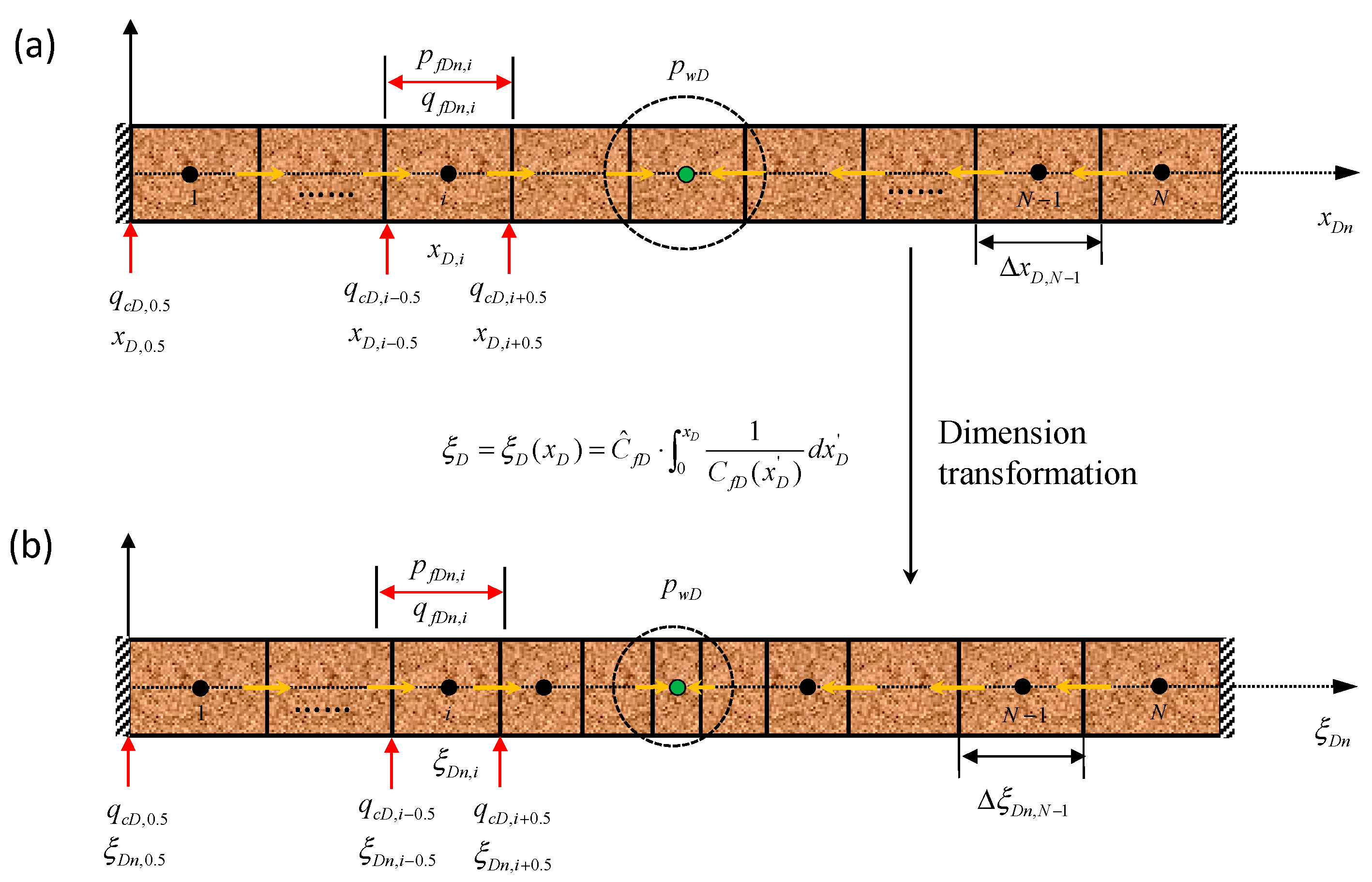
4.1. Dimension Transformation

Compared with the equation of uniform conductivity fracture described by Equations (14), (22) and (26) are subject to nonlinear equations. In the case of considering non-Darcy flow, the fracture conductivity is a function of flowing rate; in the case of considering pressure-sensitivity effect, the fracture conductivity is a function of pressure. In essence, both flow rate and pressure chang with the spatial variable. Here, we attempt to solve the problem in the same way as the linear treatment in Equation (14) by a dimension transformation, which is defined as

$$\{\begin{array}{l}{\xi }_{Dm}(x_{Dm})={\widehat{C}}_{fDm}\cdot {\displaystyle {\int }_0^{x_{Dm}}\frac{1}{C_{fDm}(x_D^{\prime })}d{x}_D^{\prime }}\\ {\widehat{C}}_{fDm}=L_{fDm}/{\displaystyle {\int }_0^{L_{fDm}}\frac{1}{C_{fDn}(x_D^{\prime })}d{x}_D^{\prime }}\end{array}$$

(27)

Then, the fracture-flow equations (Equations (22) and (26)) can be written as

$$p_{fDm}({\xi }_{Dm})=p_{fDm}({\xi }_{Dm}=0)+q_{wDm}{S}_{c,m}+\frac{2\pi }{{\widehat{C}}_{fDm}}\left({\displaystyle {\int }_0^{{\xi }_{Dm}}d\zeta {\displaystyle {\int }_0^{\zeta }{\tilde{q}}_{fDm}(\varsigma )d\varsigma }}-q_{wDm}G({\xi }_{Dm},{\xi }_{wDm})\right)$$

(28)

Equation (28) has the same form as the fracture-flow equations for a uniform-conductivity fracture with constant conductivity given by Equation (18). The difference is that the variable ξ_D is a function of the variable x_D and depends on the distribution of conductivity C_fD(x_D).

4.2. Discretization

In this study, the productivity index is achieved by discretizing the fracture panel into M segments with equal length ∆x_Di, as shown in Figure 6a. Note that the equal-length fracture segment would be transformed into an unequal-length segment after using dimension transformation, as shown in Figure 6b.

In the reservoirs, the dimensionless pressure drop on the j-th segment of the n-th fracture caused by the i-th segment of the m-th fracture is given by

$$p_{mDn,j}={\displaystyle \sum _{m=1}^{N_f}{q}_{wDm}B{D}_m^{n,j}}+{\displaystyle \sum _{m=1}^{N_f}{\displaystyle \sum _{i=1}^{M_m}{q}_{fDm,i}\mathsf{\Delta }{p}_{uDm,i}^{n,j}}}\frac{\mathsf{\Delta }{\xi }_{Dm,i}}{\mathsf{\Delta }{x}_{Dm,i}}$$

(29)

where $B{D}_m^{n,j}=I{B}_{n,j}\left(\frac{B_2{C}_{1,m}-B_1{C}_{2,m}}{A_1{B}_2-A_2{B}_1}\right)+I{D}_{n,j}\left(\frac{A_1{C}_{2,m}-A_2{C}_{1,m}}{A_1{B}_2-A_2{B}_1}\right)$, and $\mathsf{\Delta }{p}_{uDm,i}^{n,j}={\displaystyle {\int }_{x_{ofDm,i-1}}^{x_{ofDm,i}}\delta p_{uD}(u)du}$.

In the fracture, the dimensionless pressure on the j-th segment of the n-th fracture is expressed as

$$p_{wDn}-p_{fDn,j}=\frac{2\pi }{{\widehat{C}}_{fDn}}{q}_{wDn}G({\xi }_{Dn,j},{\xi }_{wDn})-[I({\xi }_{Dn,j})-I({\xi }_{wD})]-q_{wDn}{S}_{c,n}$$

(30)

where $I({\xi }_D)={\displaystyle {\int }_0^{{\xi }_D}d\zeta {\displaystyle {\int }_0^{\zeta }{\tilde{q}}_{fDn}(\varsigma )d\varsigma }}$.

According to the continuity condition that the pressure must be continuous along the fracture surface, the following conditions must hold along the fracture plane:

$$p_{mD}(x_{ofDn}+x_{Dn,j},y_{ofDn})=p_{fD}(x_{Dn,j})$$

(31)

Moreover, the sum of all the segments’ flow rate equals to the total flow rate at the m-th fracture:

$$q_{wfDm}={\displaystyle \sum _{i=1}^{M_m}\left({\tilde{q}}_{fDm,i}\frac{\mathsf{\Delta }{\xi }_{Dm,i}}{\mathsf{\Delta }{x}_{Dm,i}}\right)}$$

(32)

Combining Equations (29)–(32), we can obtain the fundamental coupled solutions by computing the apparent linear equations [36,37].

4.3. Computation Consideration

According to the previous statement, the dimensionless conductivity of C_fDn is the function of pressure p_fDn in the fracture with pressure-dependent conductivity, and the dimensionless conductivity of C_fDn is the function of flowing rate q_cDn in the fracture under non-Darcy flow. In a mathematical context, C_fDn is a function with regard to the spatial variable. At a given k-th step, if the distribution of pressure p_fDn or flowing rate q_cDn was known, C_fDn along the fracture would be obtained. Thus, the nonlinear governing equation for the (k + 1)-th step could be linearized on the assumption of known conductivity distribution on the k-th step.

In the case of considering the non-Darcy flow effect (Case 1), the formation for the k-th step yields

$$\frac{C_{fDn}}{1+{(q_{DND})}_{fn}{q}_{cDn}^{\langle k\rangle }}\frac{\partial p_{fDn}^{\langle k+1\rangle }}{\partial x_{Dn}^{}}+2\pi q_{cDn}^{\langle k+1\rangle }(x_{Dn})+2\pi q_{wDn}^{\langle k+1\rangle }H(x_{Dn},x_{wDn})=0$$

(33)

In the case of considering the pressure-dependent conductivity effect (Case 2), the formation for the k-th step yields

$$C_{fDn}(p_{fDn}^{\langle k\rangle },x_D)\frac{\partial p_{fDn}^{\langle k+1\rangle }}{\partial x_{Dn}^{}}+2\pi \left[q_{wDn}^{\langle k+1\rangle }H(x_{Dm},x_{wDm})-{\displaystyle {\int }_0^{x_{Dm}}{q}_{fDm}^{\langle k+1\rangle }(x^{\prime })d{x}^{\prime }}\right]+2\pi q_{wDn}^{\langle k+1\rangle }H(x_{Dn},x_{wDn})=0$$

(34)

The flow distribution q_fDn and pressure distribution p_fDn along the fracture at the k-th time step would be achieved based on coupled solution. Next, the calculated p_fDn was used to update the fracture conductivity (Case 1); the calculated q_cDn was used to update the fracture conductivity (Case 2). The iterative procedure is repeated until the wellbore-pressure was converged. The calculation procedure is given as follows:

• Step 1: Initial calculation, with k = 0, the fracture is assumed to be uniform (Case 1 and Case 2). By combing through Equation (29) to Equation (32), we can obtain (q_fDn)^k. The fracture pressure (p_fDn)^k (Case 1) and flowing rate (q_fDn)^k (Case 2) would be then achieved from Equation (28).
• Step 2: Calculating the pressure-sensitive conductivity C_fDn[(p_fDn)^k] (Case 1) and C_fDn[(q_cDn)^k] (Case 2) along fracture, and then transforming x_Dn into ξ_Dn based on Equation (26).
• Step 3: Solving Equation (33) with the updated C_fDn[(p_fDn)^k] to achieve (p_fDn)^k+1 and (p_wD)^k+1 in Case 1; solving Equation (34) with the updated C_fDn[(q_cDn)^k] to achieve (q_cDn)^k+1 and (p_wD)^k+1 in Case 2.
• Step 4: Terminate the iterative procedure if |(p_wD)^k+1 − (p_wD)^k|/(p_wD)^k < ε; otherwise, update pressure distribution along fracture by setting (p_fDn)k = (p_fDn)^k+1 (Case 1) and flow distribution along fracture by setting (q_cDn)^k = (q_cDn)^k+1 (Case 2), and k = k + 1 back to step 2 until the convergence is achieved.

5. Results and Sensitivity Analysis

The productivity index (PI) is defined as the ratio of the production rate to pressure drawdown, as follows:

$$J_D=\frac{\mu B}{2\pi k_{m}h}\frac{q}{p_i-p_w}=\frac{1}{p_{wD}}={\left(\frac{1}{2}\ln \frac{4A}{e^{\gamma }{C}_A{r}_{we}^2}\right)}^{-1}$$

(35)

Put another way, the dimensionless PI is the reciprocal of flow resistivity. Here, A is the drainage area, γ is the Eular constant, and C_A is the shape factor. Specially, r_we is the effective wellbore radius determined by the geometry of drainage area, well configuration, and nonlinear flow mechanism.

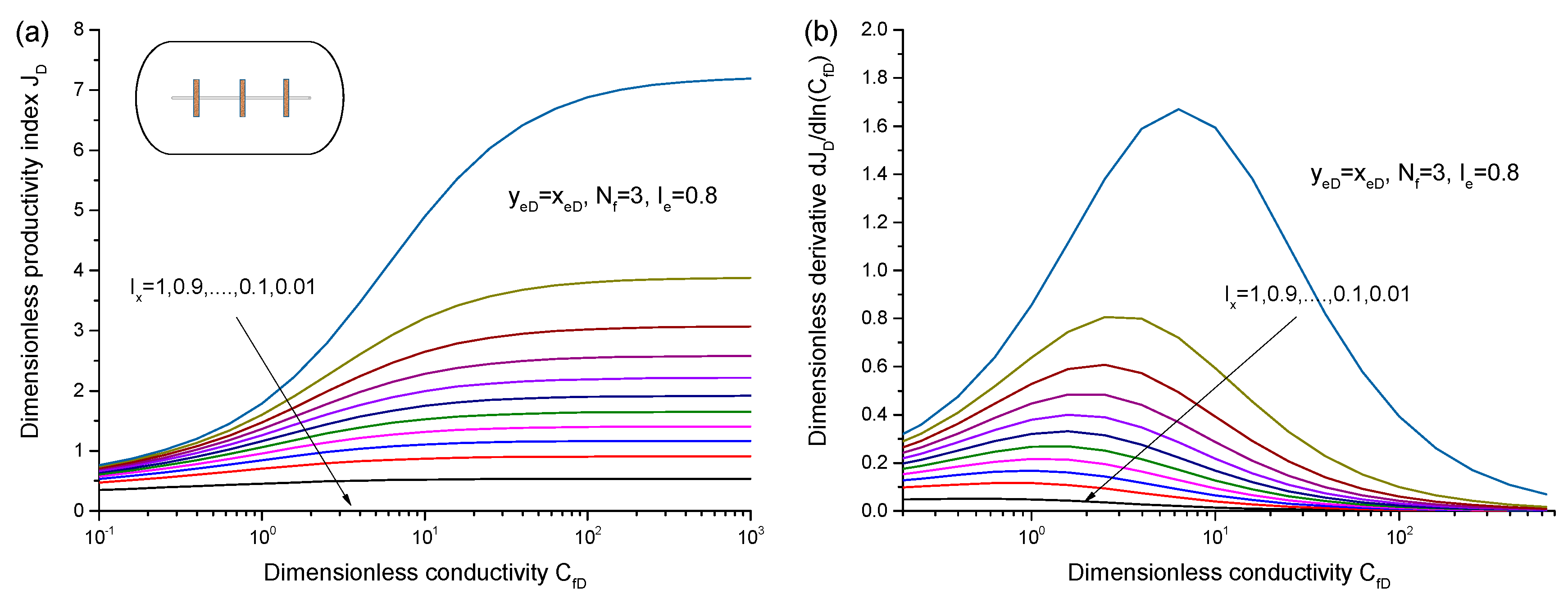
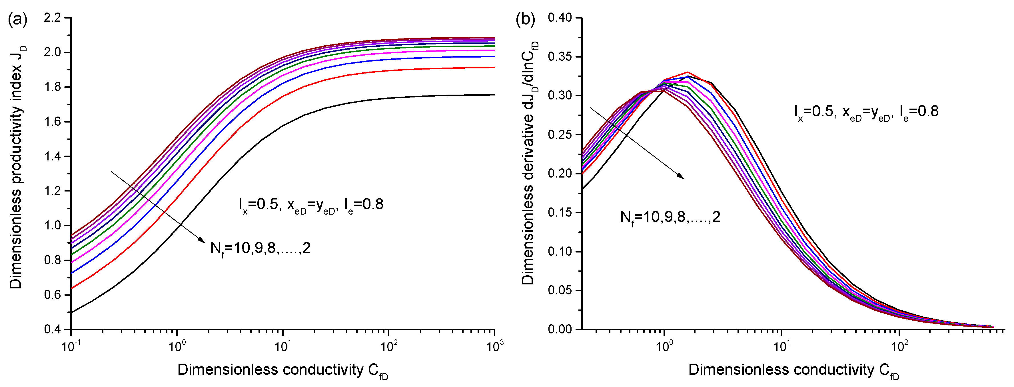
5.1. Influence of Fracture Properties on PI

In this subsection, the nonlinear flow mechanisms are firstly not taken into account, and the focus is put on the impacts of the dimensions and configuration of MFHW on PI behavior. For the purpose of discussion, homogeneous fracture properties and MFHW configuration are assumed; the fractures are evenly spaced along horizontal wellbore, and all fractures are of identical properties. As a result, the PI is mainly determined by five factors, including dimensionless conductivity (C_fD), fracture number (N_f), penetration ratio of fracture length to inner SRV width (I_x = L_f/x_e), penetration ratio of fractured horizontal wellbore to inner SRV length (I_y = D_f/y_e) (D_f is defined as the distance between two outmost fractures), and the drainage ratio of inner drainage to the whole drainage (I_e = x_e/x_R).

Figure 7 shows the effect of dimensionless conductivity on PI in the case of different penetration ratios. We further assume that the fracture is symmetrical (i.e., the fracture length on the right hand side equals to the left hand side with regard to wellbore), and all fractures are located in the center of the drainage. The fracture conductivity changes from 0.1 to 1000 (i.e., C_fD = 0.1, 0.5, 1, 5, 10, 50, 100, 500, and 1000). As shown in Figure 7a, at a given penetration ratio (I_x), PI is increased with the increase in dimensionless conductivity. However, after a certain dimensionless conductivity, the increase could be miniscule. In other words, beyond a certain dimensionless conductivity, the PI increase with conductivity essentially equals the PI decrease caused by the inner interference within the fracture. Generally, the threshold value is regarded as C_fD,threshold = 300. When the C_fD is larger than 300, there is no significant pressure drop within the fracture; the PI reaches the maximum, and does not increase with the conductivity. Figure 7b shows the PI derivative with regard to ln(C_fD) in the semi-log plot. For each given I_x, the conductivity, corresponding to the maximum PI derivative, is defined as certain conductivity. Taking I_x = 1, for example (J_Dmax = 7.25), when the derivative is at a maximum, and that the certain value is C_fD,certain = 7.5, the corresponding value of PI is J_D = 4.54. This indicates that the ratio of J_D/J_Dmax equals 62.6. This means that PI of MFHW at C_fD = 7.5 could reach 62.6% of the maximum, but PI only increases by 37.4% when the C_fD is further increased from 7.5 to 300. Therefore, the optimum dimensionless conductivity is defined to as the certain value. The optimum conductivity indicates that the inflow from the reservoir could match the outflow of the fracture. As analyzed from Figure 7b, the larger the I_x, the larger the optimum C_fD.

Figure 8 shows the effect of the number of fractures on PI behavior. As expected, the cases with a larger number exhibit a higher value of PI. That is, increasing the number contributes to an increased connected area of MHFW with the reservoirs, and an increase in the fracture–fracture interference. However, as the number of fractures increases beyond a certain number, the increase of PI could be miniscule. For example, PI increases by 8.97% when the number is increased from N_f = 2 to N_f = 3. In comparison, incremental PI would decline to 0.39% when the fracture number is further increased from N_f = 9 to N_f = 10. Overall, the effect of the increased connected area could offset the effect of the increase of fracture interference, which results from the increased fracture number. Besides, the optimum conductivity is decreased with the increase in fracture number, as shown in Figure 8b.

Figure 9 presents the effect of the ratio of inner SRV area to the whole area, i.e., I_e. Here the value that I_e = 1 means that the area of inner SRV equals to the whole drainage area. Compared with the PI that I_e = 1, the more approaching unity the value is, the larger the PI is, which is caused by the decrease of the proportion of inner SRV. Moreover, the tendency is more noticeable in the condition of high conductivity. When C_fD = 0.1, the PI at I_e = 0.5 is that J_D@Ie=0.5 = 0.45, while the PI at I_e = 1 is that J_D@Ie=1 = 0.65. Hence, the ratio of I_e = 1 to I_e = 0.5 in PI value is 1.44. As a comparison, when C_fD = 1000, the PI at I_e = 0.5 is that J_D@Ie=0.5 = 0.72, while the PI at I_e = 1 is that J_D@Ie=1 = 1.95. The ratio in PI is 2.7.

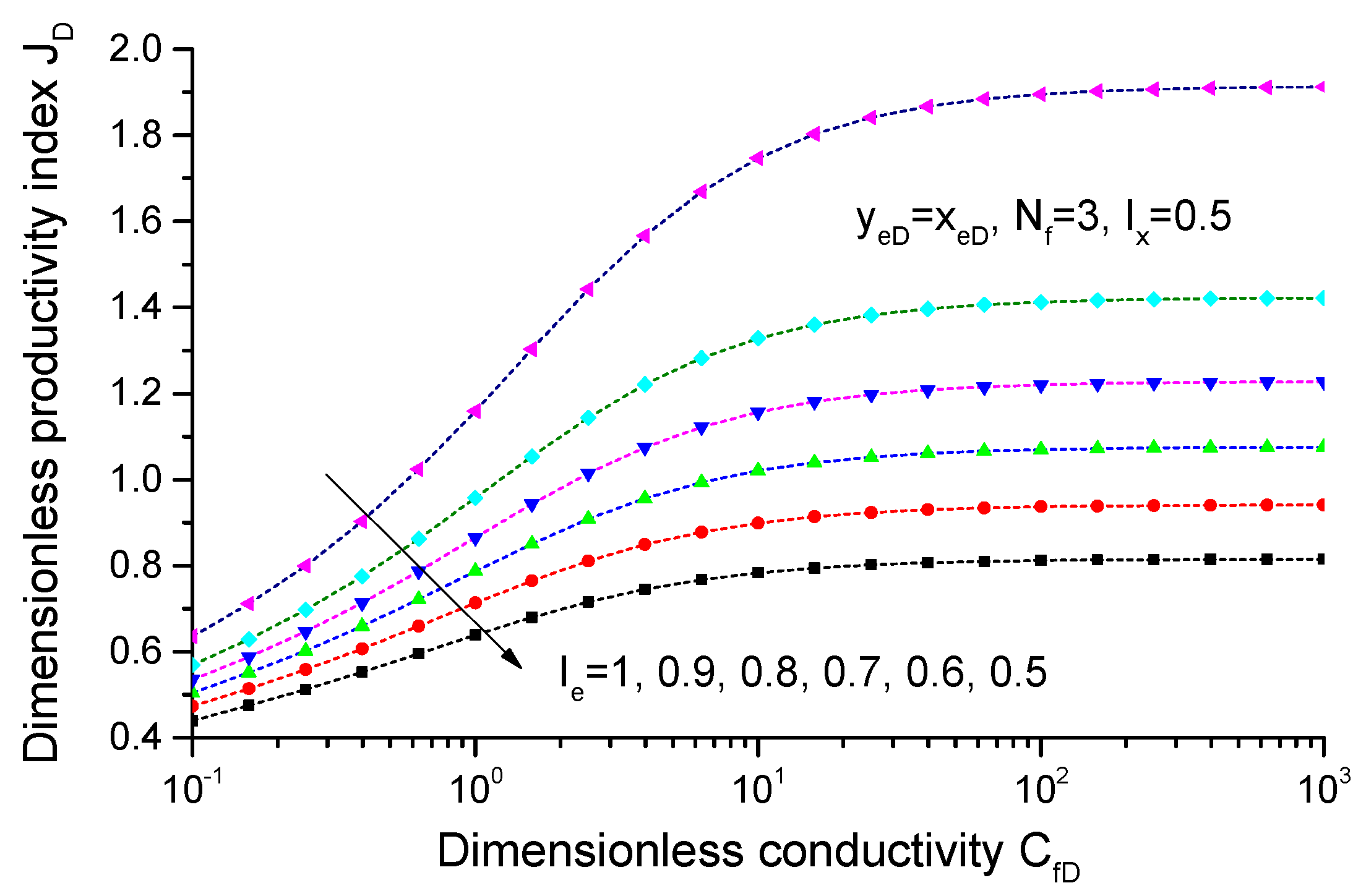
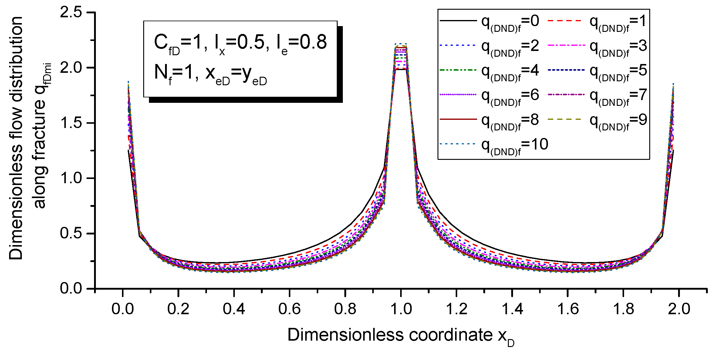
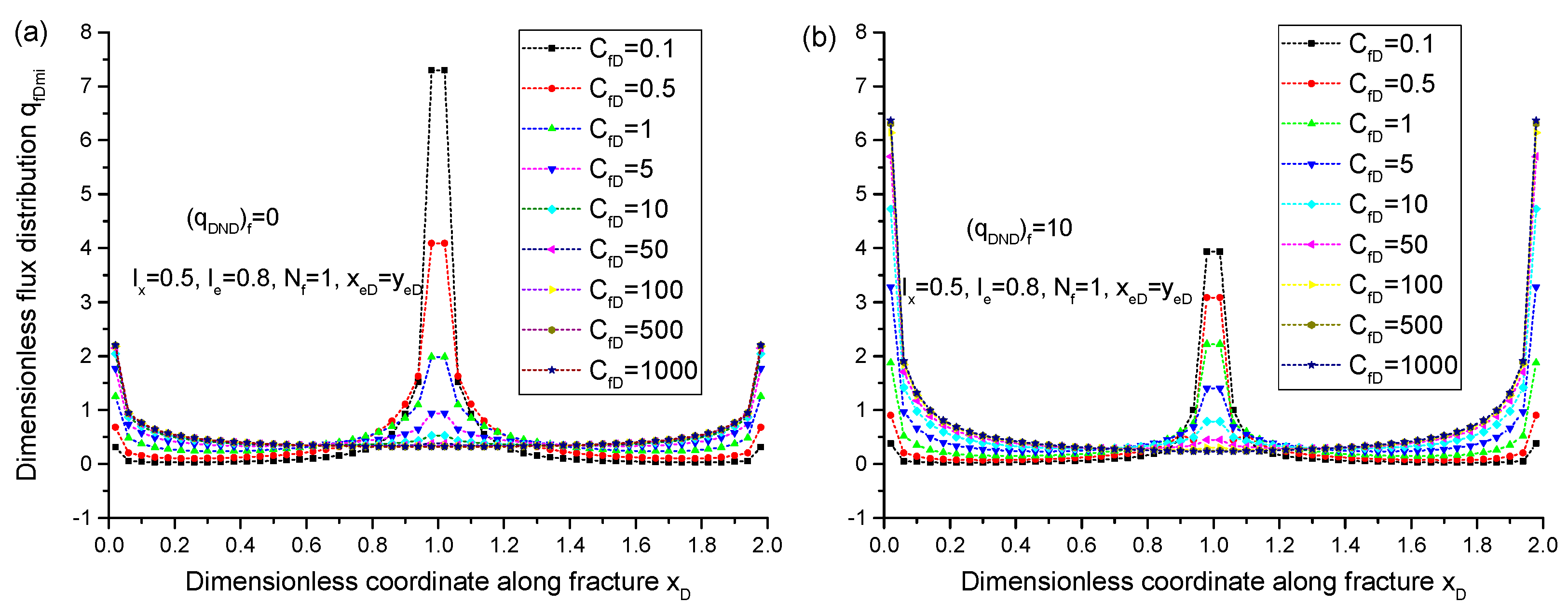
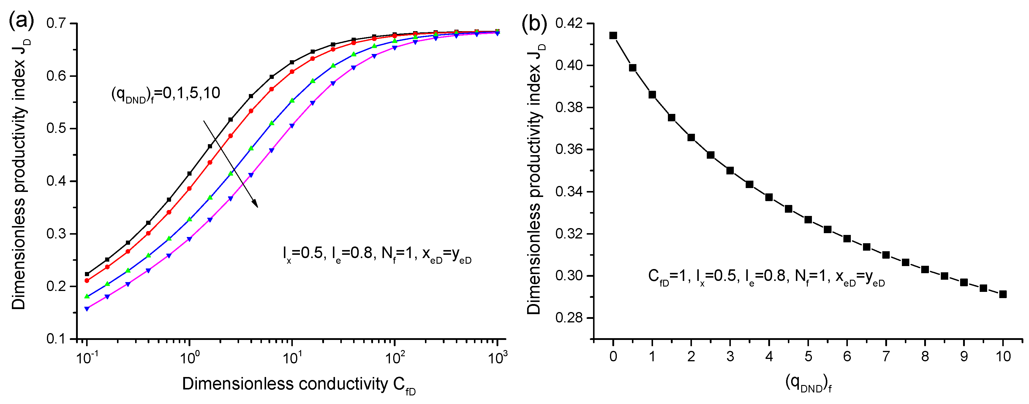
5.2. Influence of Non-Darcy Flow on PI

In this subsection, the non-Darcy flow mechanism is taken into account, and we investigate the effect of non-Darcy flow on PI behavior. Figure 10 shows the flow distribution along the fracture, where C_fD = 1. In this figure, the conductivity is set to be relatively low. It is shown that the influx density, which is defined as the influx rate per length along fracture face, is concentrated around the wellbore and fracture tips. It is noted that the concentration region of the influx density is controlled by a larger pressure drop/depletion. The variable of (q_DND)_f, defined in Equation (2), is the Forchheimer number for a given inertial factor β. When the (q_DND)_f is increased, the influx density is increasingly more concentrated towards wellbore. Put another way, an extra pressure drop is required to offset the effect of non-Darcy flow caused by the inertial force. Figure 11 presents the effect of fracture conductivity on influx-density distribution along the fracture. Without the non-Darcy effect (Forchheimer number equals zero) shown in Figure 11a, the increase in conductivity makes the distribution of fluid influx more gentle. When C_fD > 300 (i.e., infinite conductivity), which indicates that the pressure on any point in fracture panel is same as the pressure on the wellbore, the inflow flux is concentrated on the fracture tips. With the non-Darcy effect (Figure 11b), when C_fD > 1, more volume of influx fluid is concentrated on the nearby region of wellbore. The phenomenon is consistent with the characteristics given in Figure 11a. As the conductivity increases, the effect of non-Darcy flow on the distribution of inflow flux becomes weak, until the distribution of inflow flux is independent of the non-Darcy flow effect.

Figure 12 shows the effect of non-Darcy flow on PI behavior. As shown in Figure 12a, at any given conductivity, PI is the highest in the condition of (q_DND)_f = 0. PI increases with the increase of C_fD, until it reaches the maximum value (J_Dmax) at C_fD = 300. However, the increasing rate of PI is gradually slowed down with C_fD; likewise, the maximum PI is independent of (q_DND)_f. In other words, non-Darcy flow plays a negative role in determining PI for the range of low- and intermediate-conductivity (C_fD < 300), but has no effect on the maximum PI, which corresponds to the infinite conductivity. The relationship between PI and the Forchheimer number is further shown in Figure 12b. It is shown that, although PI declined with the Forchheimer number, the decreasing rate slows down.

Figure 13 shows the effect of configuration and dimension of fractures on PI behavior with the consideration of the non-Darcy flow effect. As shown in Figure 13a, PI loss in the case of a lower fracture number is relatively more noticeable than that in the case of a larger number. For example, when N_f = 2 and (q_DND)_f = 0, PI is that J_D = 0.96; when N_f = 2 and (q_DND)_f = 10, PI is that J_D = 0.75. The relative loss in PI is up to 22%, which is defined as 1 − J_D@(qDND)f=10/J_D@(qDND)f=0. In comparison, the relative loss in PI is only 9%. Figure 13b shows the penetration ratio of fracture length with respect to the inner SRV width (I_x). The effect of Forchheimer number is weaker when the I_x is relatively small, but its effect would be amplified when the I_x is relatively small. Figure 13c shows the penetration ratio of the inner SRV region with regard to whole drainage (I_e). In the small range (I_e < 0.9), the relationship between I_e and PI exhibits an approximate linear behavior. When I_e > 0.9, PI is increased rapidly with the I_e.

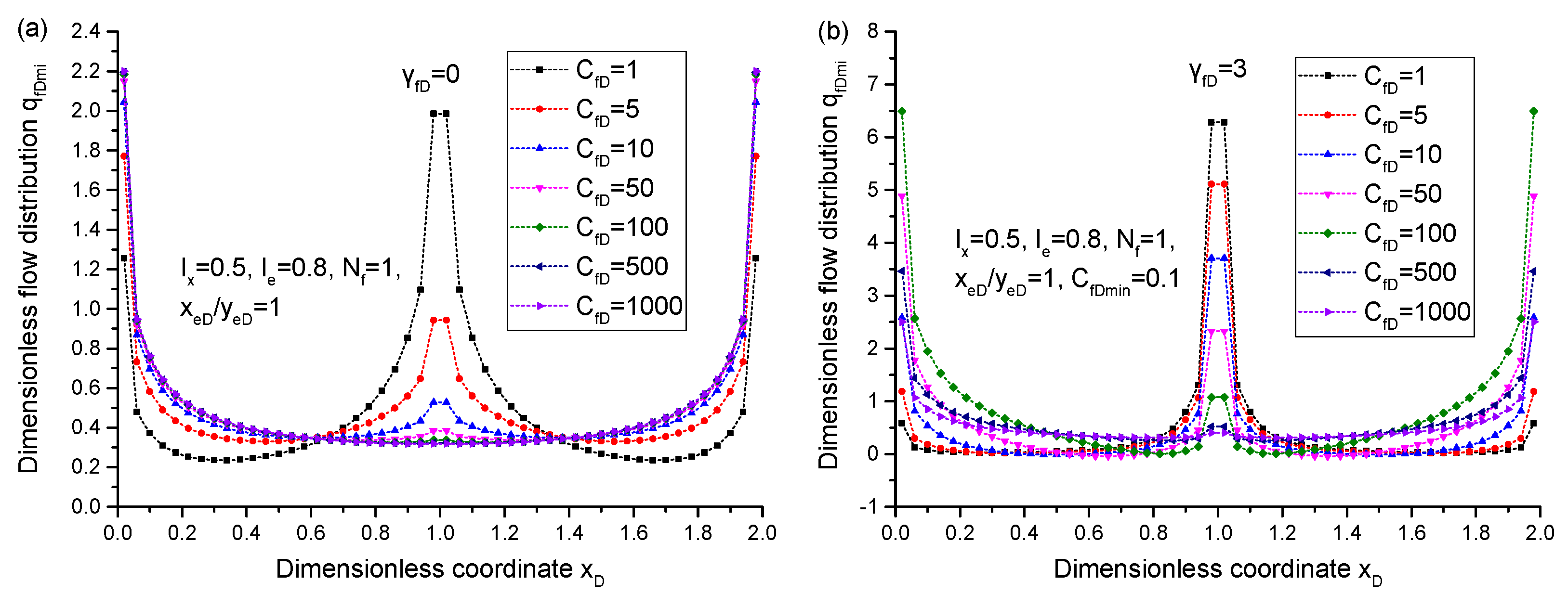
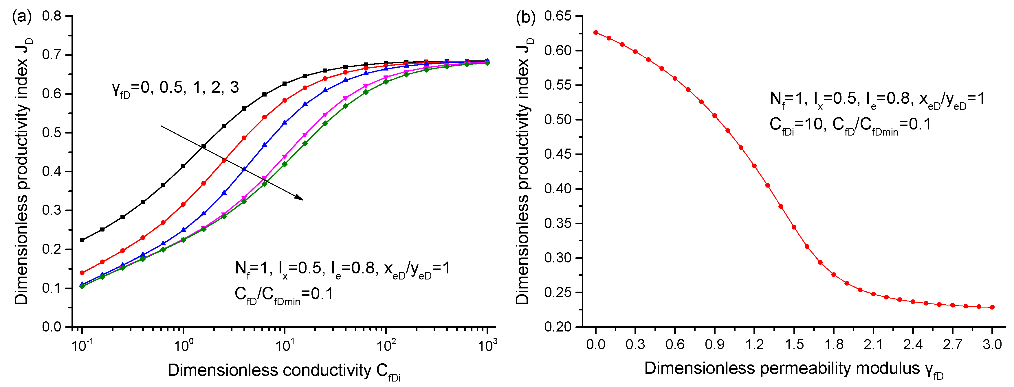
5.3. Influence of the Pressure-Sensitivity Effect on PI

The characteristic of the PI behavior is similar to the behavior of non-Darcy flow. First, Figure 14 shows the influx-distribution along the fracture with the consideration of the pressure-sensitivity effect. Compared with the nonsensitive case (Figure 14a), more influx density is distributed around the wellbore in the sensitive case (Figure 14b), and the tendency would be more remarkable with the decrease of the conductivity. The reason is explained in that the apparent conductivity is degraded and the flow resistance is consequently increased, which is caused by the closing of the fracture under the influence of rock compaction.

Figure 15 shows the effect of pressure sensitivity on PI behavior. The intensity is measured by the dimensionless variable γ_fD. As shown in Figure 15a, the effect of pressure sensitivity on PI becomes weak with the increase of the conductivity. When the magnitude of the conductivity reaches the level of infinite conductivity, the effect of pressure sensitivity is almost neglected. As expected, as presented in Figure 15b, PI declines until the minimum with the increasing γ_fD, and corresponding γ_fD is defined as the threshold. Meanwhile, the decreasing rate slows down. For example, if C_fD = 1, PI reaches the minimum J_Dmin when γ_fDthreshold = 1.2; if C_fD = 10, PI reaches the minimum J_Dmin when γ_fDthreshold = 2.7. Thus, a larger conductivity contributes to a larger γ_fDthreshold.

Figure 16 shows the effect of configuration and dimension of fractures on PI in the consideration of pressure sensitivity in the fracture. The overall features are similar to the case of considering non-Darcy flow, so we will not rewrite again.

6. Conclusions

We derived a new steady-state productivity model for a multi-fractured horizontal well in a reservoir with pseudo-elliptical boundary. We summarize some important findings as follows:

• PI increases with the increase of C_fD, until it reaches the maximum (J_Dmax) at C_fD = 300.
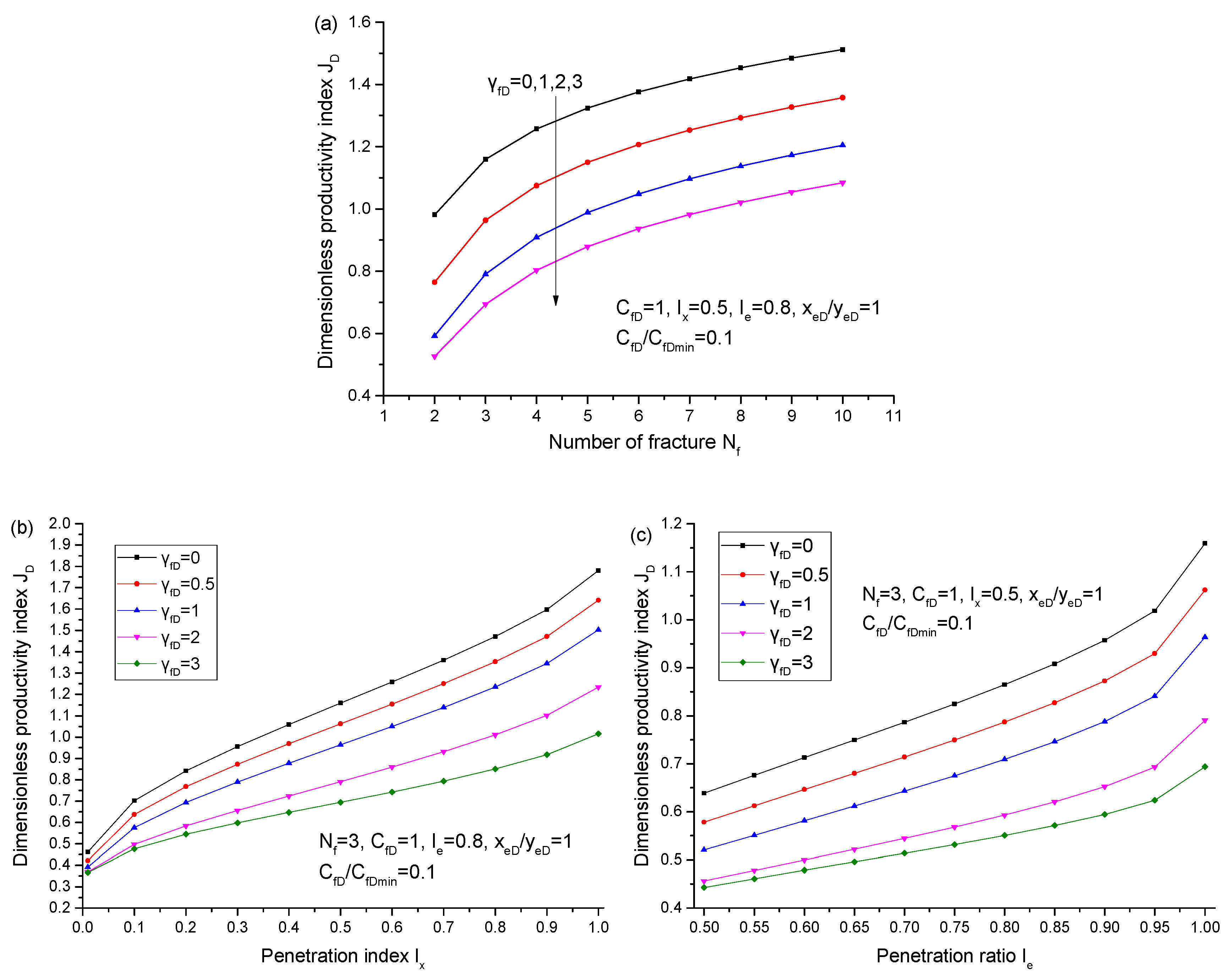
• PI is deteriorated under the influence of nonlinear flow mechanisms. With the consideration of non-Darcy flow, for the small range of the penetration ratio of the inner SRV region with regard to whole drainage (I_e < 0.9), the relationship between I_e and PI exhibits an approximately linear behavior. When I_e > 0.9, PI is increased rapidly with the I_e.
• With the consideration of pressure sensitivity, the apparent fracture is degraded from the initial conductivity to the minimal conductivity, which is caused by fracture closure. As a result, an extra pressure drop is acquired to offset the conductivity degradation, and PI would be declined to the minimal PI.
• The disadvantage dimensions of fracture (such as small conductivity, penetration ratio, and less fractures) contribute to severe pressure depletion, while, in turn, the severe pressure depletion will strengthen the effect of the nonlinear flow mechanism on PI behavior.
• If the conductivity in the fracture reaches the level of infinite conductivity, the influence of nonlinear flow mechanism on PI could be neglected.

References

- Clarkson, C.R.; Bustin, R.M.; Seidle, J.P. Production-data analysis of single-phase (gas) coalbed-methane wells. SPE Reserv. Eval. Eng. 2007, 3, 312–341. [Google Scholar] [CrossRef]
- Wang, J.H.; Wang, X.D.; Dong, W.X. Rate decline curves analysis of multiple-fractured horizontal wells in heterogeneous reservoirs. J. Hydrol. 2017, 553, 527–539. [Google Scholar] [CrossRef]
- Deng, J.; Zhu, W.Y.; Ma, Q. A new seepage model for shale gas reservoir and productivity analysis of fractured well. Fuel 2014, 124, 232–240. [Google Scholar] [CrossRef]
- Clarkson, C.R. Production data analysis of unconventional gas wells: Review of theory and best practices. Int. J. Coal Geol. 2013, 109–110, 101–146. [Google Scholar] [CrossRef]
- Zhang, Q.; Su, Y.L.; Wang, W.D.; Lu, M.; Ren, L. Performance analysis of fractured wells with elliptical SRV in shale reservoirs. J. Nat. Gas Sci. Eng. 2017, 45, 380–390. [Google Scholar] [CrossRef]
- Wang, J.L.; Wei, Y.S.; Luo, W.J. A unified approach to optimize fracture design of a horizontal well intercepted by primary- and secondary-fracture networks. SPE J. 2019, 24, 1270–1287. [Google Scholar] [CrossRef]
- Al-Rbeawi, S. Productivity-index behavior for hydraulically fractured reservoirs depleted by constant production rate considering transient-state and semisteady-state conditions. SPE Prod. Oper. 2018, 33. [Google Scholar] [CrossRef]
- Warren, J.E.; Root, P.J. The behavior of naturally fractured reservoirs. SPE J. 1963, 3, 245–255. [Google Scholar] [CrossRef]
- Obinna, E.D.; Hassan, D. A model for simultaneous matrix depletion into natural and hydraulic fracture networks. J. Nat. Gas Sci. Eng. 2014, 16, 57–69. [Google Scholar]
- Stalgorova, E.; Mattar, L. Analytical model for unconventional multifractured composite systems. SPE Reserv. Eval. Eng. 2013, 16, 246–256. [Google Scholar] [CrossRef]
- Al-Ghamdi, A.; Chen, B.; Behmanesh, H.; Qanbari, F.; Aguilera, R. An improved triple-porosity model for evaluation of naturally fractured reservoirs. SPE Reserv. Eval. Eng. 2011, 8, 397–404. [Google Scholar] [CrossRef]
- Karimi-Fard, M.; Durlofsky, L.J. A general gridding, discretization, and coarsening methodology for modeling flow in porous formations with discrete geological features. Adv. Water Resour. 2016, 96, 354–372. [Google Scholar] [CrossRef]
- Xu, Y.; Cavalcante Filho, J.S.A.; Yu, W. Discrete-fracture modeling of complex hydraulic-fracture geometries in reservoir simulators. SPE Reserv. Eval. Eng. 2017, 20, 403–422. [Google Scholar] [CrossRef]
- Li, L.Y.; Lee, S.H. Efficient field-scale simulation of black oil in a naturally fractured reservoir through discrete fracture networks and homogenized media. SPE Reserv. Eval. Eng. 2008, 8, 750–758. [Google Scholar] [CrossRef]
- Cinco-Ley, H.; Samaniego, F.; Dominguez, N. Transient pressure behavior for a well with a finite-conductivity vertical fracture. Soc. Pet. Eng. J. 1978, 8, 254–265. [Google Scholar]
- Wang, J.L.; Jia, A.L.; Wei, Y.S.; Qi, Y.D. Approximate semi-analytical modeling of transient behavior of horizontal well intercepted by multiple pressure-dependent conductivity fractures in pressure-sensitive reservoir. J. Pet. Sci. Eng. 2017, 153, 157–177. [Google Scholar] [CrossRef]
- Wang, J.L.; Jia, A.L.; Wei, Y.S. A general framework model for simulating transient response of a well with complex fracture network by use of source and Green’s function. J. Nat. Gas Sci. Eng. 2018, 55, 254–275. [Google Scholar] [CrossRef]
- Zhou, W.T.; Banerjee, R.; Poe, B. Semianalytical production simulation of complex hydraulic-fracture networks. SPE J. 2013, 19, 6–18. [Google Scholar] [CrossRef]
- Kuchuk, F.; Biryukov, D. Pressure-transient behavior of continuously and discretely fractured reservoirs. SPE Reserv. Eval. Eng. 2014, 17, 82–97. [Google Scholar] [CrossRef]
- Al-Rbeawi, S. The optimal reservoir configuration for maximum productivity index of gas reservoirs depleted by horizontal wells under Darcy and non-Darcy flow conditions. J. Nat. Gas Sci. Eng. 2018, 49, 179–193. [Google Scholar] [CrossRef]
- Chen, Z.M.; Liao, X.W.; Zhao, X.L.; Lyu, S.; Zhu, L. A comprehensive productivity equation for multiple fractured vertical well with non-linear effects under steady-state flow. J. Pet. Sci. Eng. 2017, 149, 9–24. [Google Scholar] [CrossRef]
- Li, J.; Guo, B.; Gao, D.; Ai, C. The effect of fracture-face matrix damage on productivity of fractures with infinite and finite conductivities in shale-gas reservoirs. SPE Drill. Complet. 2012, 9, 347–353. [Google Scholar] [CrossRef]
- Prats, M.; Raghavan, R. Finite horizontal well in a uniform-thickness reservoir crossing a natural fracture normally. SPE J. 2013, 10, 982–992. [Google Scholar] [CrossRef]
- Tahmasebi, P.; Kamrava, S. A pore-scale mathematical modeling of fluid-particle interactions: Thermo-hydro-mechanical coupling. Int. J. Greenh. Gas Control 2019, 83, 245–255. [Google Scholar] [CrossRef]
- Zhang, X.M.; Tahmasebi, P. Effects of grain size on deformation in porous media. Transp. Porous Media 2019, 129, 321–341. [Google Scholar] [CrossRef]
- Zhang, X.M.; Tahmasebi, P. Micromechanical evaluation of rock and fluid interactions. Int. J. Greenh. Gas Control 2018, 76, 266–277. [Google Scholar] [CrossRef]
- Guppy, K.H.; Cinco-Ley, H.; Ramey, H.J. Effect of non-Darcy flow on the constant-pressure production of fractured wells. Soc. Pet. Eng. J. 1981, 12, 390–400. [Google Scholar] [CrossRef]
- Wu, Y.S.; Li, J.F.; Ding, D.; Wang, C.; Di, Y. A generalized framework model for simulation of gas production in unconventional gas reservoir. In Proceedings of the SPE Reservoir Simulation Symposium, The Woodlands, TX, USA, 18–20 February 2013. [Google Scholar]
- Lin, J.; Zhu, D. Predicting well performance in complex fracture systems by slab source method. In Proceedings of the SPE Hydraulic Fracturing Technology Conference, The Woodlands, TX, USA, 6–8 February 2012. [Google Scholar]
- Pedroso, C.A.; Correa, A.C. A new model of a pressure-dependent-conductivity hydraulic fracture in a finite reservoir: Constant rate production case. In Proceedings of the Latin American and Caribbean Petroleum Engineering Conference, Rio de Janeiro, Brazil, 30 August–3 September 1997. [Google Scholar]
- Zhang, Z.; He, S.L.; Liu, G.; Guo, X.; Mo, S. Pressure buildup behavior of vertically fractured wells with stress-sensitive conductivity. J. Pet. Sci. Eng. 2014, 122, 48–55. [Google Scholar] [CrossRef]
- Yao, S.S.; Zeng, F.H.; Liu, H. A semi-analytical model for hydraulically fractured wells with stress-sensitive conductivities. In Proceedings of the SPE Unconventional Resources Conference, Calgary, AB, Canada, 5–7 November 2012. [Google Scholar]
- Biryukov, D.; Kuchuk, F.J. Transient pressure behavior of reservoirs with discrete conductive faults and fractures. Transp. Porous Media 2012, 95, 239–268. [Google Scholar] [CrossRef]
- Rasoulzadeh, M.; Kuchuk, F.J. Pressure transient behavior of high-fracture-density reservoirs (dual-porosity models). Transp. Porous Media 2019, 127, 222–243. [Google Scholar] [CrossRef]
- Kuchuk, F.J.; Habashy, T. Pressure behavior of laterally composite reservoirs. SPE Form. Eval. 1997, 3, 47–56. [Google Scholar] [CrossRef]
- Luo, W.J.; Tang, C.F. A semianalytical solution of a vertical fractured well with varying conductivity under non-Darcy-flow condition. SPE J. 2015, 20, 1028–1040. [Google Scholar] [CrossRef]
- Luo, W.J.; Tang, C.F.; Feng, Y. Mechanism of fluid flow along a dynamic conductivity fracture with pressure-dependent permeability under constant wellbore pressure. J. Pet. Sci. Eng. 2018, 166, 465–475. [Google Scholar] [CrossRef]
© 2020 by the authors. Licensee MDPI, Basel, Switzerland. This article is an open access article distributed under the terms and conditions of the Creative Commons Attribution (CC BY) license (http://creativecommons.org/licenses/by/4.0/).
Share and Cite
Cao, M.; Xiao, H.; Wang, C. Productivity-Index Behavior for a Horizontal Well Intercepted by Multiple Finite-Conductivity Fractures Considering Nonlinear Flow Mechanisms under Steady-State Condition. Energies 2020, 13, 2015. https://doi.org/10.3390/en13082015
Cao M, Xiao H, Wang C. Productivity-Index Behavior for a Horizontal Well Intercepted by Multiple Finite-Conductivity Fractures Considering Nonlinear Flow Mechanisms under Steady-State Condition. Energies. 2020; 13(8):2015. https://doi.org/10.3390/en13082015
Chicago/Turabian StyleCao, Maojun, Hong Xiao, and Caizhi Wang. 2020. "Productivity-Index Behavior for a Horizontal Well Intercepted by Multiple Finite-Conductivity Fractures Considering Nonlinear Flow Mechanisms under Steady-State Condition" Energies 13, no. 8: 2015. https://doi.org/10.3390/en13082015
APA StyleCao, M., Xiao, H., & Wang, C. (2020). Productivity-Index Behavior for a Horizontal Well Intercepted by Multiple Finite-Conductivity Fractures Considering Nonlinear Flow Mechanisms under Steady-State Condition. Energies, 13(8), 2015. https://doi.org/10.3390/en13082015