A Novel Topology Optimization Approach for Flow Power Loss Minimization Across Fin Arrays

Abstract

Fin arrays are widely utilized in many engineering applications, such as heat exchangers and micro-post reactors, for higher level of fluid–solid contacts. However, high fluid pressure loss is reportedly the major drawback of fin arrays and a challenge for pumping supply, particularly at micro-scales. Previous studies also indicate that fin shapes, spacing and alignment play an important role on the overall pressure losses. Therefore, we present a numerical tool to minimize pressure losses, considering the geometrical aspects related to fin arrays. In this regard, a density-based topology optimization approach is developed based on the pseudo-spectral scheme and Brinkman penalization in 2D periodic domains. Discrete sensitives are derived analytically and computed at relatively low cost using a factorization technique. We study different test cases to demonstrate the flexibility, robustness and accuracy of the present tool. In-line and staggered arrays are considered at various Reynolds numbers and fluid–solid volume fractions. The optimal topologies interestingly indicate a pressure loss reduction of nearly $53.6\%$ compared to circular fins. In passive optimization test examples, the added solid parts reduced pressure loss of a circular fin ($9\%$) by eliminating the flow separation and filling the wake region.

1. Introduction

Fin array (FA) structural designs are broadly utilized in many devices which require a significant level of fluid–solid contact. FAs are composed of uniformly distributed and identical structures with a repeated pattern and large surface area to volume ratios, suitable for high performance and compact heat or mass transfer applications, such as micro heat-exchangers [1] and micro-reactors [2]. The promising performance of FAs, however, comes with the price of high pressure drop [3,4], which can be very challenging for pumping supply, particularly at micro-scales or applications with space limitations. Previous numerical and experimental studies on isothermal single-phase flow across fin arrays suggest that geometrical attributes, such as fin shape, alignment and pitch-space play a significant role on the total flow pressure drop [5,6,7,8]. Therefore, in this work, we utilize a density-based topology optimization approach to find the optimal fin geometries which minimize flow pressure drop (power loss), considering the designing aspects of fin arrays, and develop a numerical tool for this purpose.

Towards minimizing pressure drops by improving fin geometry, topology optimization (TO) [9] is fundamentally a superior approach, primarily for its ultimate ability to deal with complex geometries. TO was originally developed for optimizing solid structures [10,11], but soon after was extended to optimization of fluid flow systems [12,13,14,15], and in the past decade, new TO developments have shown very promising performances in various applications, such as hydrothermal systems [16,17], fluid–structure interaction (FSI) problems [18,19] and microfluidic mixers [20,21]. Various TO approaches have been previously developed focusing on isothermal flow power loss minimization for internal (channel) flow [13,15,22] and external flow problems [12,18], where the latter is the case for flow past an array of fins, considered in the present work. In this context, Borrvall and Petersson [12] were pioneer to achieve optimal hydrodynamic shapes, similar to rugby balls, corresponding to a prescribed volume constraint and featuring minimized Stokes flow power dissipation. Guest and Prévost [23] developed a Darcy–Stokes topology optimization model for very low Reynolds flows, equipped with an inverse homogenization method to design porous material micro-structures. Targeting maximum flow permeability, they interestingly achieved porous materials with periodic micro-structures; however, they reported some numerical difficulties regarding the choice of initial mWaterial distribution. Kondoh et al. [24] investigated drag minimization and lift maximization via a convenient body force integration objective function and successfully achieved optimal airfoils for low to moderate Reynolds numbers. Lundgaard et al. [25] studied optimal topologies of a plate obstacle with six different objective functions such as minimum flow dissipated energy and structural compliance, using a robust density-based TO formulation, and comprehensively discussed the critical implementation details. Zhou et al. [26] more recently proposed a combined shape and topology optimization method with a boundary-smoothing regularization technique to guarantee a stable convergence, and achieved physically meaningful optimal hydrodynamic shapes, submerged in Stokes flow.

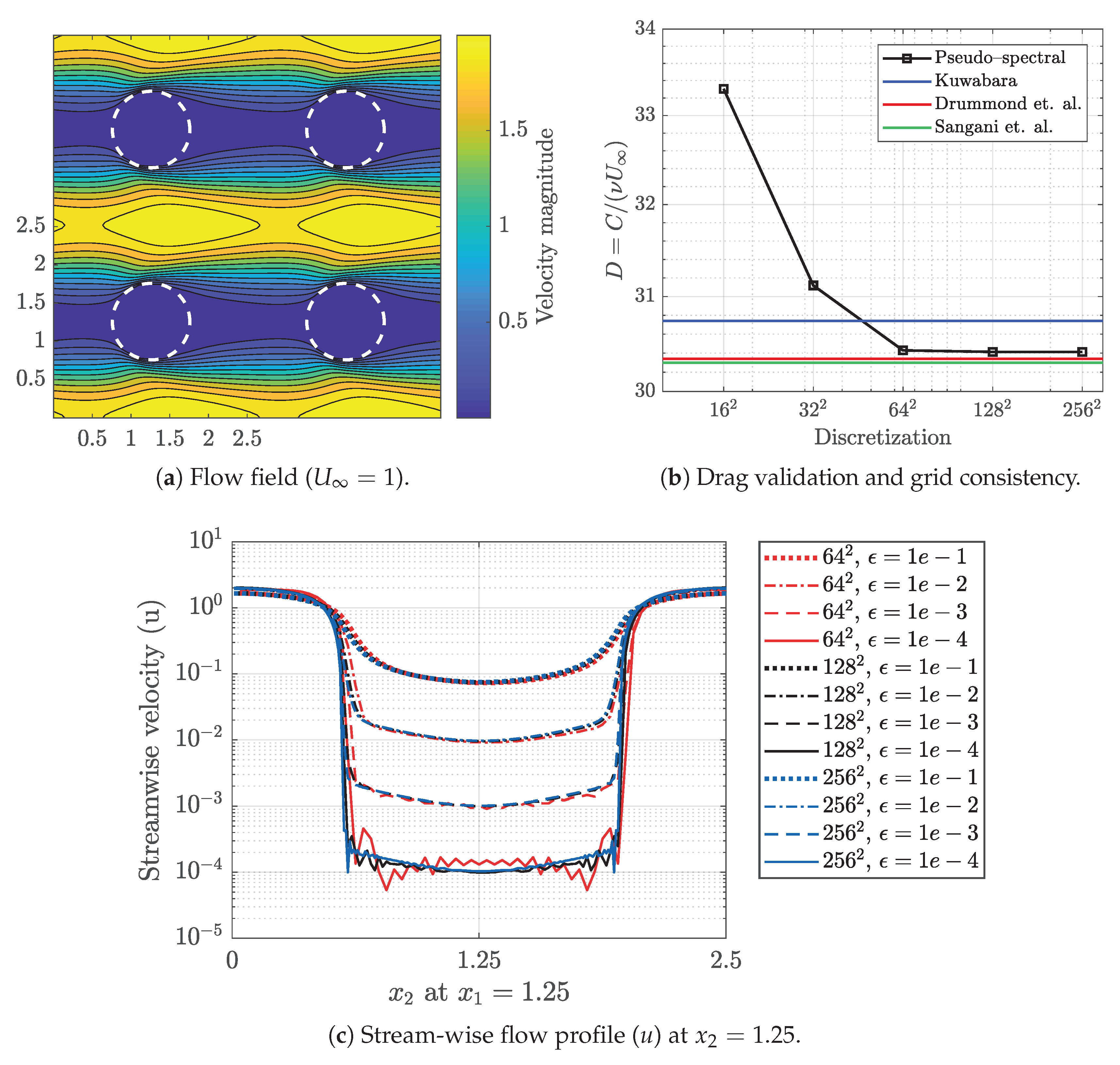
In this work, we present a novel TO approach for drag minimization of fin arrays in isothermal two-dimensional (2D) steady flows. We assume a doubly periodic computational domain, including a single design region for individual fins. This assumption is well consistent with the repeated flow pattern across uniform fins at low Reynolds numbers, and significantly saves computational efforts. In addition, single periodic design domain, in favor of topology optimization, requires fixed number of design variables for fin topologies independent FA size, and allows full pressure-velocity fields decomposition which leads to reduced number of state variables by factor of 2/3. For the numerical flow solution, we utilize highly accurate pseudo-spectral scheme, equipped with Brinkman volume penalization technique. Pseudo-spectral scheme is based on discrete Fourier approximation of the periodic solution on a uniform grid, which provides a desirable level of accuracy with less grid points compared to other numerical techniques such as finite difference methods [27]. Moreover, because of the global approximation of the flow solution, the accuracy at a solid–fluid boundary is well satisfactory [28], especially when the boundary is moving over a fixed uniform grid, as it is the case for optimization process.

For gradient-based optimization, we describe the analytical sensitivity analysis for the pseudo-spectral method, and validate its accuracy using finite differencing method. We use GCMMA [29] as the optimizer and implement a convenient factorization technique which substantially reduces numerical efforts with respect to computing the required sensitivities at a satisfactory accuracy level. The remainder of the paper is organized as follows: In Section 2, we concisely introduce pseudo-spectral scheme used for penalized Navier-Stokes, and discuss the computational model, boundary conditions and etc. We present in Section 3 the topology optimization formulation and derive the sensitivity analysis followed by finite differencing verification. In Section 4, we study three optimization examples to qualitatively and quantitatively investigate flexibility, robustness, accuracy and overall performance of the present TO approach in drag minimization of fin arrays, at different Reynolds number and solid volume sized. Section 5 summarizes the key features and state-of-the-art achievements we investigated using the present tool.

2. Flow Modeling and Numerical Method

2.1. Penalized Navier-Stokes

The flow system is modeled using the incompressible Naviers–Stokes equations on a 2D doubly periodic square domain, $\mathsf{\Omega }$, as

$$\frac{\partial \mathbf{u}}{\partial t}+\mathbf{u}·\nabla \mathbf{u}+\frac{1}{\rho }\nabla P-\nu \Delta \mathbf{u}=0$$

(1)

and

$$\nabla ·\mathbf{u}=0,$$

(2)

where $\mathbf{u}$ is the velocity vector, P the hydrodynamic pressure, $\nu$ the kinematic viscosity and $\rho$ the density of fluid. We employ Brinkman penalization method to define a solid material distribution within the computational domain $\mathsf{\Omega }$ [28,30,31]. By using this technique, a no permeable solid zone (${\mathsf{\Omega }}_s$) is formed simply by modifying the Navier–Stokes equation with the added penalization term, instead of explicit solid zone with solid–fluid boundary definition. Therefore, in favor of numerical methods, the computational mesh conveniently remains fixed and re-meshing is not required during formation or movement of solid zones. The penalized Navier-Stokes form of Equation (1) is

$$\frac{\partial {\mathbf{u}}_{ϵ}}{\partial t}+{\mathbf{u}}_{ϵ}·\nabla {\mathbf{u}}_{ϵ}+\frac{1}{\rho }\nabla P-\nu \Delta {\mathbf{u}}_{ϵ}-\frac{1}{ϵ}\chi \left(\mathbf{x}\right){\mathbf{u}}_{ϵ}=0$$

(3)

$$\nabla ·{\mathbf{u}}_{ϵ}=0$$

(4)

where ${\mathbf{u}}_{ϵ}$ is the approximated solution of Equations (1) and (2) for fluid velocity, $ϵ$ the penalization parameter, which controls the flow permeability into solid zones and the dimensionless spatial function $\chi \left(\mathbf{x}\right)$, ranging from 0 to 1, is the penalization function. Brinkman penalization technique is the base tool for density-based topology optimization that we use in the present flow system. Solid material distributions are simply controlled by $\chi \left(\mathbf{x}\right)$ function, independent of mesh treatment. Here, $\chi =1$ imposes full penalization to model a solid material zone. $\chi =0$ has no penalization effect, therefore flow equations are solved for fluid material. Any values of $0<\chi <1$ treat as porous medium, meaning a permeable solid zone with a continuous permeability level controlled by $\chi$. As it will be discussed in the following section, the penalization function $\chi \left(\mathbf{x}\right)$ is the only varying parameter for handling solid zones during fin topology optimization, and is referred to design parameters.

Regarding the accuracy of the penalization technique, the approximated solution of (3) and (4) is proved to converge to the solution of (1) and (2) with the error norm bounded by

$$\left|\right|\mathbf{u}-{\mathbf{u}}_{ϵ}\left|\right|\le C{ϵ}^{1/2},$$

(5)

meaning smaller the $ϵ$, smaller the penalization error [32]. The boundary conditions in this flow model are defined as

$$\left\{\begin{array}{cc}\mathbf{u}=0\hfill & \mathrm{in}{\mathsf{\Omega }}_s,\mathrm{and}\mathrm{on}\partial {\mathsf{\Omega }}_s\hfill \\ \mathbf{u}\mathrm{is}\mathrm{double}\mathrm{periodic}\hfill & \mathrm{on}\mathsf{\Omega },\hfill \end{array}\right.$$

(6)

and the mean flow velocity is ${\mathbf{u}}_{\infty }$ at upstream.

The pressure term in Equation (3) is eliminated by utilizing an orthogonal projector $\mathbb{P}$ onto the divergence-free space (see [33]), using the Helmholtz decomposition providing a unique solution for a space-periodic domain [34]. Equations (3) and (4) after the projection become

$$\frac{\partial {\mathbf{u}}_{ϵ}}{\partial t}+\mathbb{P}({\mathbf{u}}_{ϵ}·\nabla {\mathbf{u}}_{ϵ})-\nu \Delta {\mathbf{u}}_{ϵ}-\frac{1}{ϵ}\chi \left(\mathbf{x}\right){\mathbf{u}}_{ϵ}=0,$$

(7)

where $\mathbb{P}$ is an orthogonal projection operator. Note that the projected ${\mathbf{u}}_{ϵ}$ automatically satisfies Equation (4), and in what follows, the $ϵ$ subscription is removed for brevity.

2.2. Numerical Methods

To numerically approximate the solution of Equation (7), we utilize the powerfull and accurate pseudo-spectral scheme [28]. In this numerical approach, the flow velocity at point $\mathbf{x}=(x_1,x_2)$ and time t is approximated using Fourier series as

$$\mathbf{u}(x_1,x_2,t)=\sum _{k\in Z^2}{\mathbf{u}}_k\left(t\right)\exp \left[\begin{array}{c}2\pi i\left(\frac{k_1{x}_1+k_2{x}_2}{L}\right)\end{array}\right]$$

(8)

where $x_1,x_2\in \left[0L\right]$, L is the size of the physical domain ($\mathsf{\Omega }$), $k_1,k_2\in \left\{-\frac{N}{2}+1,-\frac{N}{2}+2,\dots ,\frac{N}{2}\right\}$ are discretized points in 2D Fourier domain (wave numbers), N is an even number equal to the number of discretization points in each direction, and ${\mathbf{u}}_k$ is the corresponding value of $\mathbf{u}$ in the Fourier space. The 2D discrete Fourier transform of Equation (8) in the matrix form is simply performed by

$$\mathbf{U}=H{\mathbf{U}}_k{H}^T$$

(9)

where $\mathbf{U}$ and ${\mathbf{U}}_k$ are N-by-N discretized velocity field matrices in the physical and Fourier domain, respectively. H is the 2D discrete Fourier transform matrix, of which matrix elements $h_{l,m}$ are

$$h_{l,m}=cos\left(\frac{2\pi lm}{N}\right)-i[sin\left(\frac{2\pi lm}{N}\right)]$$

(10)

Back to the Navier-Stokes equations, the Equation (7) using a proper divergence-free projection operator $\mathbb{P}$ becomes

$$\frac{\partial \mathbf{u}}{\partial t}=\mathbf{u}\times \mathbf{\omega }+\nu \Delta \mathbf{u}+\frac{1}{ϵ}\chi \left(\mathbf{x}\right)\mathbf{u}\doteq \mathsf{\Lambda }(\mathbf{u},\chi \left(\mathbf{x}\right)),$$

(11)

where $\mathbf{\omega }$ is the flow vorticity. The divergence-free projection is conveniently performed in the Fourier space for each discretization node as

$${\left[\begin{array}{c}u\\ v\end{array}\right]}_{div-free}={(k_1^2+k_2^2)}^{-1}\left[\begin{array}{cc}{k}_2^2& -k_1{k}_2\\ -k_1{k}_2& k_1^2\end{array}\right]\left[\begin{array}{c}u\\ v\end{array}\right].$$

(12)

And $\mathsf{\Lambda }=({\mathsf{\Lambda }}_1,{\mathsf{\Lambda }}_2)$ is defined as the time derivative of the velocity field; hence, we expect $\mathsf{\Lambda }=0$ if the flow is steady-state. Elements of matrices $\left[{\mathsf{\Lambda }}_1\right]$ and $\left[{\mathsf{\Lambda }}_2\right]$ are computed in few steps (see [35] for more details). We first discretize $\mathsf{\Omega }$, N times in each direction and then compute an N-by-N matrix of vorticity field in physical domain by

$$\left[\mathbf{\omega }\right]=\mathrm{real}\left(\overline{H}(K_1\circ \left(H\mathbf{V}{H}^T\right)-K_2\circ \left(H\mathbf{U}{H}^T\right)){\overline{H}}^T\right)$$

(13)

where $\overline{H}$ is the complex conjugate transpose of H, $K_1$ and $K_2$ are wave number matrices with normalized $k_1$ and $k_2$ in each rows and columns, respectively and ∘ is the Hadamard matrix product operation. Next, we compute the convective, viscous and penalization terms of Equation (11) in Fourier space by

$$\begin{array}{cc}\widehat{\left[{\mathsf{\Lambda }}_1\right]}=\hfill & \nu (K_1\circ K_1+K_2\circ K_2)\circ \left(H\mathbf{U}{H}^T\right)-\hfill \\ \hfill & H(\frac{1}{ϵ}\left[\chi \right]\circ \mathbf{U}-\mathbf{V}\circ \left[\mathbf{\omega }\right])H^T\hfill \\ \widehat{\left[{\mathsf{\Lambda }}_2\right]}=\hfill & \nu (K_1\circ K_1+K_2\circ K_2)\circ \left(H\mathbf{V}{H}^T\right)-\hfill \\ \hfill & H(\frac{1}{ϵ}\left[\chi \right]\circ \mathbf{V}+\mathbf{U}\circ \left[\mathbf{\omega }\right])H^T,\hfill \end{array}$$

(14)

where $\left[\chi \right]$ is also an N-by-N matrix of penalization function values defined on all nodes over domain $\mathsf{\Omega }$. Using the divergence–free projection $\mathbb{P}$ of Equation (12) we get

$$\begin{array}{c}\widehat{\left[\mathsf{\Lambda }\right]}=\mathbb{P}\left(\left[\widehat{\mathsf{\Lambda }}\right]\right)\hfill \end{array}$$

(15)

which automatically satisfies the conservation of mass. In final step, we need to perform inverse transform to find $\mathsf{\Lambda }$ in the physical space

$$\begin{array}{c}\left[{\mathsf{\Lambda }}_1\right]=\mathrm{real}\left(\overline{H}\left[\widehat{{\mathsf{\Lambda }}_1}\right]{\overline{H}}^T\right)\hfill \\ \left[{\mathsf{\Lambda }}_2\right]=\mathrm{real}\left(\overline{H}\left[\widehat{{\mathsf{\Lambda }}_2}\right]{\overline{H}}^T\right)\hfill \end{array}$$

(16)

It should be noted that the discrete Fourier transforms in Equations (13), (14) and (16) could be computed either directly or using the efficient fast Fourier transform algorithms, e.g., FFTW library [36]. It is also noticeable that so far we derived the values of $\mathsf{\Lambda }$ using the basic matrix operations. We will show in the following that this approach significantly simplifies the discrete sensitivity analysis of the numerical method, required for gradient-based optimization.

2.3. Drag Force: Computation and Validation

The drag force, which we will consider as the objective function for optimization, is simply computed by integrating the Brinkman penalization term over the solid zones [31] by

$${\mathbf{C}}_{drag}=\frac{1}{ϵ}\underset{{\mathsf{\Omega }}_s}{\int }\mathbf{u}\mathrm{d}\mathbf{x}\cong \frac{1}{ϵ}d{x}^2\sum _{l,m=1}^N{U}_{l,m}^s{\chi }_{l,m}.$$

(17)

where $U^s$ is the stream-wise component of $\mathbf{u}$ and $dx=L/N$ the domain discretization size.

Reliability of the pseudo-spectral scheme together with the Brinkman penalization technique, as well as the accuracy of the drag force computed from Equation (17) have been previously studied and approved for both 2D and 3D simulations at moderate to high Reynolds numbers [37,38]. However, for low Reynolds number flows, we need to verify the accuracy and perform the grid consistency study. In this regard, we solved a flow problem for an in-line cylindrical fin configuration with the pitch-to-diameter ratio of 0.4 at $Re=5$ and set upstream velocity $U_{\infty }$ to 1. Figure 1a demonstrates the periodic flow field across a circular array. Note that only four computational domains (2-by-2) are plotted in this case to demonstrate the periodicity in the flow field. The white dashed line represents the penalized domain (${\mathsf{\Omega }}_s$) wherein $\chi =1$. We also perform a series of simulations by varying the domain discretization size (N) in order to check grid consistency and compare the calculated drag with previous studies.

Figure 1b suggests the drag force exerted on a single fin in an in-line array, and Figure 1c illustrates the stream-wise flow velocity profile in the cross section of the fin with respect to discretization size and Brinkman penalization parameter ($ϵ$). In penalization technique, solid structures are teated as porous media with permeability controlled by penalization parameter. This implies that the velocities in solid zones never become actually zero, but they are damped. From Figure 1c we observe that smaller the $ϵ$, smaller the flow seepage is. However, by reducing $ϵ$ we observe oscillating velocity profile due to a known Gibbs phenomenon. Gibbs phenomenon appears in spectral methods when a sharp discontinuity exists in the solution. We also see that this phenomenon is controlled in higher resolutions. Considering the accuracy and consistency of the computed drag force (with respect to the previous studies), sufficiently damped flow seepage in the solid zone, as well as the controlled Gibbs oscillations, we find the ${128}^2$ resolution and $ϵ={10}^{-3}$ adequately precise and satisfying values in this work.

It should be noted that the drag force by integration of Equation (17) is calculated at a very low computational cost, in the absence of explicit knowledge of solid–fluid boundary. This is a great advantage of penalization technique in favor of topology optimization where the geometry varies during the optimization process and an accurate drag values at intermediate steps are required and explicit boundary tracking is not always straightforward.

3. Topology Optimization

The required hydrodynamic power supply (${\dot{W}}_{hydro}$) to compensate the fluid pressure drop is computed by

$${\dot{W}}_{hydro}=\frac{\dot{m}}{\rho }\Delta P,$$

(18)

where the required power is linearly proportional to pressure drop, assuming that the flow rate ($\dot{m}$) and density are constant. Moreover, the total pressure drop is a function of hydrodynamic drag forces exerted on fins. Therefore, to minimize the required pumping power supply, we aim to establish a hydrodynamic drag minimization problem, given by:

$$\begin{array}{cccc}\hfill & \underset{\gamma }{\mathrm{minimize}}\hfill & \hfill & C\left(\chi \right(\gamma ),\mathbf{u}(\chi \left(\gamma \right)\left)\right)\hfill \\ \hfill & \mathrm{subject}\mathrm{to}\hfill & \hfill & V^{\ast }\le V\left(\chi \left(\gamma \right)\right)\hfill \\ \hfill & \hfill & 0\le {\gamma }_i\le 1\forall {\gamma }_i\in {\mathsf{\Omega }}_D.\hfill \end{array}$$

(19)

where C is the drag force and the objective function, V the fin volume (cross-section area), $V^{\ast }$ the minimum desired fin volume, and $\gamma$ the vector of design variables in the design domain ${\mathsf{\Omega }}_D\subseteq \mathsf{\Omega }$. Design variables ${\gamma }_i$’s are uniformly defined on entire the design domain, located at each discretization point ${\mathbf{x}}_i$. The topology function $\chi$ is then calculated at each point ${\mathbf{x}}_i$ from the corresponding design variable ${\gamma }_i$ using a continuous interpolation function [12], as

$$\chi \left(\gamma \right)=\frac{\gamma }{1+I_a(1-\gamma )},$$

(20)

where, $I_a$ is a parameter which controls the interpolation convexity, i.e., the transition from fluid to solid for intermediate design variables ($0<\gamma <1$).

For the present gradient-based optimization problem we use the globally convergent method of moving asymptotes (GCMMA) [29] optimizer. GCMMA algorithm is particularly developed for TO problems with large number of design variables, which is up to ${128}^2$ in our test cases. We adjust the algorithm with the standard settings, however, the move step parameter is reduced to 0.1 and the maximum number of sub-cycles is limited to 10 sub-iterations. In practice, we observed a very satisfactory performance by using GCMMA, in terms of efficiency as well as accuracy and robustness.

3.1. Sensitivity Analysis

The goal of sensitivity analysis is to precisely calculate changes of a desirable function caused by varying the design variables. This step is essential for gradient-based topology optimization, especially when there are very large number of design variables such that finite difference approximation of the sensitivities become significantly expensive. In our particular case, we need to accurately compute the drag force gradients with respect to $\gamma$’s, at a reasonable computational cost.

The objective function in Equation (19), computed by Equation (17), is a function of velocity field and the topology (penalization) function and is concisely defined as

$$C=C\left(\mathbf{u}\right(\chi ),\mathbf{v}(\chi ),\chi ).$$

(21)

And we derive the total derivative of C with respect to the vector of design variables, $\gamma$, using the chain rule of differentiation by

$$\frac{DC}{D\gamma }=\frac{\partial C}{\partial \chi }\frac{\partial \chi }{\partial \gamma }+\frac{\partial C}{\partial u}\frac{Du}{D\chi }\frac{D\chi }{D\gamma }+\frac{\partial C}{\partial v}\frac{Dv}{D\chi }\frac{D\chi }{D\gamma }.$$

(22)

We note that the simplicity of Equation (17) allows a convenient calculation of partial derivatives $\frac{\partial C}{\partial \chi }$, $\frac{\partial C}{\partial u}$ and $\frac{\partial C}{\partial v}$ at a very low cost. We also calculate $\frac{D\chi }{D\gamma }$ simply from Equation (20). The total derivatives $\frac{Du}{D\chi }$ and $\frac{Dv}{D\chi }$ represent the total rate of change in flow velocity field with respect to change of design variables and are generally difficult to derive analytically and expensive to compute. For pseudo-spectral scheme, however, it is rather straightforward to derive those derivatives by analytical differentiation of the discrete solution of Equation (11). In this regard, we integrate the solution of Equation (11) in time using Euler method and derive it for discretized $\mathbf{u}$ at time step $n+1$ by

$$\begin{array}{c}\hfill u_{n+1}=u_n+\Delta t{\mathsf{\Lambda }}_1(u_n,v_n,\chi )\mathrm{and}{u}_0=u_{init}\\ \hfill v_{n+1}=v_n+\Delta t{\mathsf{\Lambda }}_2(u_n,v_n,\chi )\mathrm{and}{v}_0=v_{init},\end{array}$$

(23)

where $\Delta t$ is the time step size, chosen based on CFL condition for numerical stability. Next, by taking the derivative of Equation (23) directly with respect to $\chi$, we obtain

$$\begin{array}{c}\hfill \frac{D{u}_{n+1}}{D\chi }=\frac{D{u}_n}{D\chi }+\Delta t[\frac{\partial {\mathsf{\Lambda }}_{1,n}}{\partial \chi }+\frac{\partial {\mathsf{\Lambda }}_{1,n}}{\partial u}\frac{D{u}_n}{D\chi }+\frac{\partial {\mathsf{\Lambda }}_{1,n}}{\partial v}\frac{D{v}_n}{D\chi }],\frac{D{u}_0}{D\chi }=0,\\ \hfill \frac{D{v}_{n+1}}{D\chi }=\frac{D{v}_n}{D\chi }+\Delta t[\frac{\partial {\mathsf{\Lambda }}_{2,n}}{\partial \chi }+\frac{\partial {\mathsf{\Lambda }}_{2,n}}{\partial u}\frac{D{u}_n}{D\chi }+\frac{\partial {\mathsf{\Lambda }}_{2,n}}{\partial v}\frac{D{v}_n}{D\chi }],\frac{D{v}_0}{D\chi }=0,\end{array}$$

(24)

where the Jacobian matrices ($\frac{\partial {\mathsf{\Lambda }}_1}{\partial u},\cdots$) are derived directly from differentiation of Equations (13)–(16). For instance, we compute the matrix of $\partial {\mathsf{\Lambda }}_1/\partial \chi$, using the chain rule of differentiation by

$$\frac{\partial {\mathsf{\Lambda }}_1}{\partial \chi }=\frac{\partial {\mathsf{\Lambda }}_1}{\partial \widehat{{\mathsf{\Lambda }}_1}}(\frac{\partial \widehat{{\mathsf{\Lambda }}_1}}{\partial \widehat{{\mathsf{\Lambda }}_1}}\frac{\partial \widehat{{\mathsf{\Lambda }}_1}}{\partial \chi }+\frac{\partial \widehat{{\mathsf{\Lambda }}_1}}{\partial \widehat{{\mathsf{\Lambda }}_2}}\frac{\partial \widehat{{\mathsf{\Lambda }}_2}}{\partial \chi }),$$

(25)

where $\partial \widehat{{\mathsf{\Lambda }}_1}/\partial \chi$ and $\partial \widehat{{\mathsf{\Lambda }}_2}/\partial \chi$ are simply calculated from differentiating Equation (14).

Direct Computation of $\frac{Du}{D\chi }$ and $\frac{Dv}{D\chi }$, as derived in Equation (24), is very expensive, but we employ a few techniques that substantially reduces the computational costs for it. In this regards, we first reformulate Equation (24) to obtain an unified matrix form, as

$${\left[\begin{array}{c}\frac{Du}{D\chi }\\ \frac{Dv}{D\chi }\end{array}\right]}_{n+1}=\Delta t{\left[\begin{array}{c}\frac{\partial {\mathsf{\Lambda }}_1}{\partial \chi }\\ \frac{\partial {\mathsf{\Lambda }}_2}{\partial \chi }\end{array}\right]}_n+(\Delta t{\left[\begin{array}{cc}\frac{\partial {\mathsf{\Lambda }}_1}{\partial u}& \frac{\partial {\mathsf{\Lambda }}_1}{\partial v}\\ \frac{\partial {\mathsf{\Lambda }}_2}{\partial u}& \frac{\partial {\mathsf{\Lambda }}_2}{\partial v}\end{array}\right]}_n+\mathbb{I}){\left[\begin{array}{c}\frac{Du}{D\chi }\\ \frac{Dv}{D\chi }\end{array}\right]}_n,$$

(26)

or in a succinct form such as

$${\mathbb{D}}_{n+1}={\mathbb{A}}_n+{\mathbb{B}}_n\times {\mathbb{D}}_n.$$

(27)

To save computational effort, we compute ${\mathbb{A}}_n$ and ${\mathbb{B}}_n$ matrices with the converged flow solutions of Equation (23) only once. Since the initial guess for velocity is always fixed, ${\mathbb{D}}_0$ equals zero. Therefore, we obtain

$$\left\{\begin{array}{c}{\mathbb{D}}_1=\mathbb{A}+\mathbb{B}\times {\mathbb{D}}_0=\mathbb{A}\hfill \\ {\mathbb{D}}_2=\mathbb{A}+\mathbb{B}\times {\mathbb{D}}_1=\mathbb{A}+\mathbb{B}\times \mathbb{A}\hfill \\ {\mathbb{D}}_3=\mathbb{A}+\mathbb{B}\times {\mathbb{D}}_2=\mathbb{A}+\mathbb{B}\times \mathbb{A}+{\mathbb{B}}^2\times \mathbb{A}\hfill \\ \cdots \hfill \\ {\mathbb{D}}_m=(\mathbb{I}+\mathbb{B}+{\mathbb{B}}^2+\cdots +{\mathbb{B}}^{m-1})\times \mathbb{A}.\hfill \end{array}\right.$$

(28)

We further simplify Equation (28) using algebraic factorization. For steps which m equals to $2^k$ (k is a natural number), we can derive

$$\begin{array}{cc}\hfill {\mathbb{D}}_m& =(\mathbb{I}+\mathbb{B})\times (\mathbb{I}+{\mathbb{B}}^2)\times (\mathbb{I}+{\mathbb{B}}^4)\times \cdots \times (\mathbb{I}+{\mathbb{B}}^{2^{k-1}})\times \mathbb{A}\hfill \\ \hfill & =\left[\prod _{J=0}^{k-1}(\mathbb{I}+{\mathbb{B}}^{2^J})\right]\times \mathbb{A}\hfill \\ \hfill & ={\mathbb{R}}_k\times \mathbb{A}.\hfill \end{array}$$

(29)

Therefore, instead of iterating over Equation (26) for every single step of m, we only compute ${\mathbb{D}}_m$ at $m=1,2,4,\cdots ,2^k$, which leads to an extremely fast convergence. More precisely, for solution of Equation (26), $2^k$ matrix additions and multiplications are required if $m=2^k$; on the other hand, only k matrix additions and $2k+1$ multiplications are required for Equation (29). 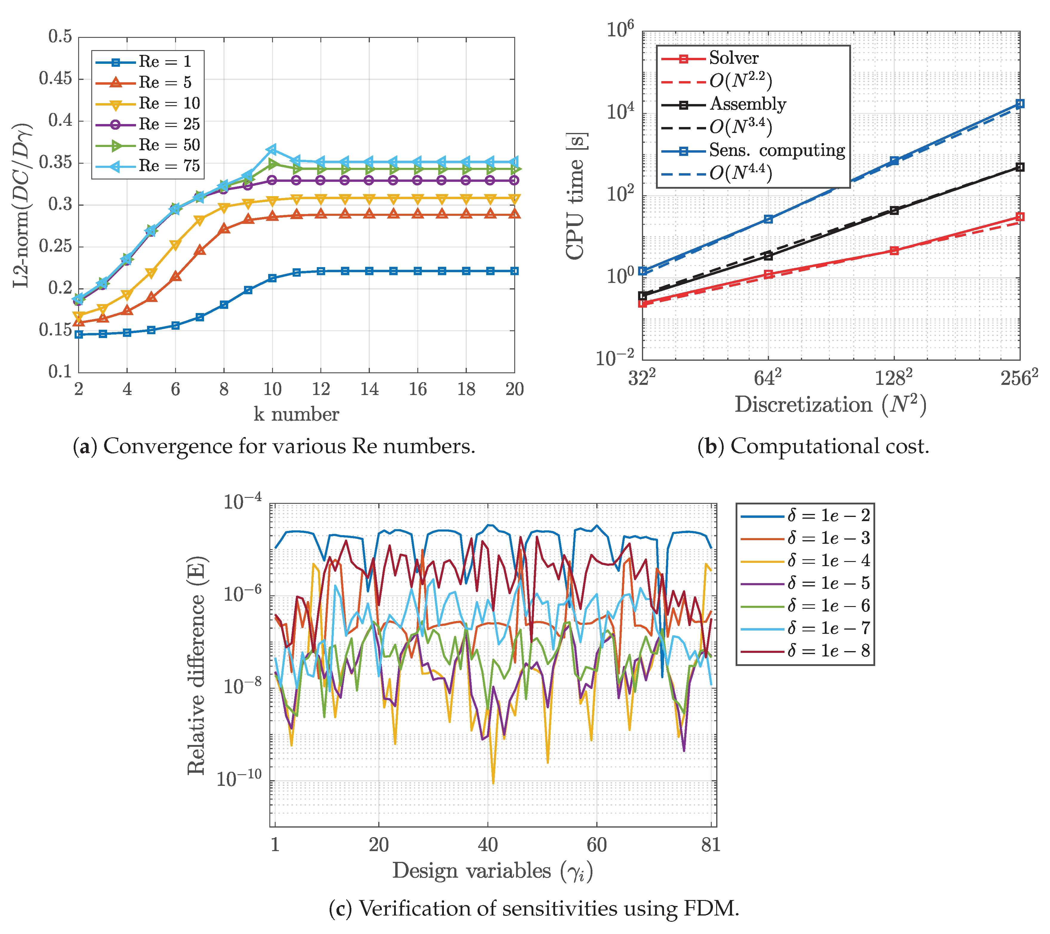Numerical experiments, as shown in Figure 2a, suggest that $DC/D\gamma$ reasonably converges after only $k=12$ iteration steps for Reynolds numbers up to 75, where the flow remains laminar and steady-state.

3.2. Accuracy Verification and Cost of Sensitivity Computation

A crucial step for a gradient-based topology optimization approach is the accuracy of the sensitivities. In our case, sensitivities are derived based on an analytical differentiation which is exact, however, they are computed via an iterative factorization technique (Equations (27)–(29)). Therefore the accuracy of the converged sensitivities as well as the implementation correctness have to be verified. For this purpose, we approximate the sensitivities $DC/D{\gamma }_i$ using central differencing finite difference method (FDM), as the reference of comparison, via:

$${\frac{DC}{D{\gamma }_i}}^{FDM}=\frac{C({\gamma }_i+\delta )-C({\gamma }_i-\delta )}{2\delta }$$

(30)

where $\delta$ is the design variable perturbation. Then, the relative error between analytical and FDM sensitivities for design variable i is computed by

$$E_i=\frac{{DC/D{\gamma }_i}^{FDM}-{DC/D{\gamma }_i}^{analytic}}{{DC/D{\gamma }_i}^{FDM}}$$

(31)

Figure 2c illustrates the relative errors for a $9\times 9$ design space for various perturbation sizes. We can observe a perfect match between the obtained sensitivities for $\delta ={10}^{-5}$, which verifies the accuracy to a desirable level of $E<{10}^{-6}$.

For every single iteration of optimization steps, we need to calculate objective function via pseudo-spectral solver (Equations (13)–(16)) and sensitivities corresponding to the current state of design variables. Computing sensitivities mainly consists of two parts: (a) calculation/assembly of matrices in Equation (26), and (b) computing Equation (29) in an iterative manner. Figure 2b illustrates an averaged CPU time required to compute the three stated tasks on a 14-core processor, for various problem sizes. The computational cost of pseudo-spectral solver is reasonably low and scales roughly with total number of grid points. The main computational burden is dedicated to computing Equation (29), since Jacobian matrices sizes are $N^2\times N^2$ and grow rapidly by problem size N. Using our current code implementation and for $N=128$ size, which is sufficiently accurate as discussed before, it takes roughly 15–20 min for a single optimization iteration on a multi-core processor and requires up to 18 GB of memory in total.

We point out that we derived the discrete sensitives of the pseudo-spectral fluid solver via an analytical process and direct differentiation. However, in general, for other complex flow solvers such as finite volume method (FVM) with an iterative SIMPLE scheme [42], exact sensitivity derivation is not straightforward [15], and often this crucial task is delivered to automatic differentiation (AD) tools [43,44]. AD tools are accurate to the machine precision, but they normally require significant amount of memory and are sometimes very time consuming. In addition, computing the required sensitivities are performed using discrete adjoint method [45]. This is a commonly utilized approach to reduce computational costs independent of number of design variables. Adjoint method, however, requires solving a linear system of equations, while the present approach does not require solving any system of equations, its cost is also independent of design variable numbers and relies only on the basic matrix operation, which could be easily implemented and computed via parallel processing.

4. Optimization Results and Discussion

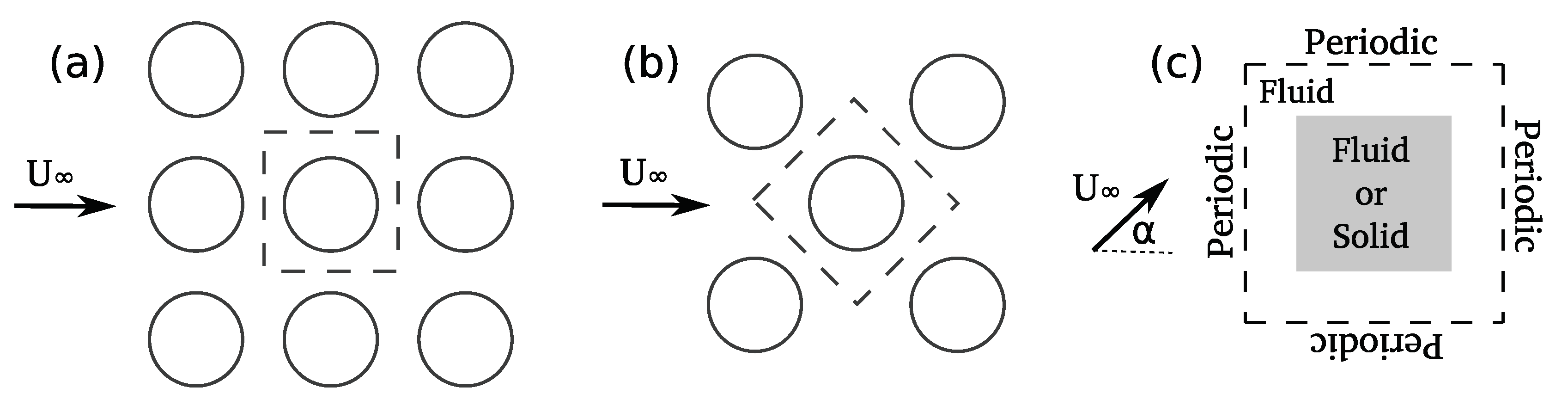
In this section, we study several test problems to investigate the utility and flexibility of the present topology optimization approach for fin array drag (pressure loss) minimization. As illustrated in the schematic Figure 3a,b, we consider two fin array configurations: in-line, and staggered (${45}^{\circ }$) alignments. Figure 3c presents our computational model as well as the design space. The dashed square area represents the periodic computational domain $\mathsf{\Omega }=L\times L$, and the gray area shows the design domain ${\mathsf{\Omega }}_D=L_D\times L_D$. We take $L_R=L/2$ as the characteristic length, and circular fins as the reference design. Length of the design domain ($L_D$) varies between $L_R$ and L, depending on the simulation case. For consistency among different simulations and fin shapes, we always calculate Reynolds number based on the characteristic length $L_R$. In addition, for sake of convenience, we rotate upstream flow direction by ${45}^{\circ }$ to model staggered array instead of rotating computational domain (compare Figure 3a,b).

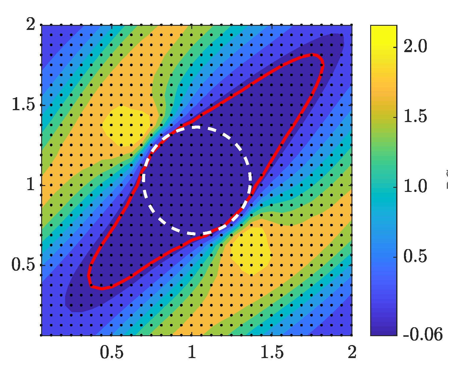
Since we employ a gradient-based optimization approach, it is important to analyze the sensitivities we obtained from Section 3.1, prior to studying the optimization results. Figure 4 demonstrates the contour field of hydrodynamic drag sensitivities for a staggered circular fin array ($\alpha ={45}^{\circ }$). The dashed white circle defines the penalized (no permeable) solid zone, and the red line indicates $DC/D\gamma =0$ contour level. Inside the red enclosure sensitivities are negative, i.e., $DC/D\gamma <0$. Negative gradient zones are of critical importance, because by increasing design variables $\gamma$ or equivalently the solid zones, drag force decreases. We can then anticipate the potentials for new topologies such that produce less drags. It should be noted that the red contour does not necessarily represent the final optimum fin geometry. The sensitivity field which is plotted here corresponds to the circular fin before optimization, and by changing the fin geometry during the optimization process, sensitivities change as well. What we can also expect from sensitivity analysis is that the optimum topology should match the zero gradient contour for unconstrained volume optimization, i.e., no unfilled negative gradient zones should be left.

In the following, we study different example problems, to investigate the utility of our topology optimization approach for fin array drag minimization. In the first case, we begin with optimizing circular in-line and staggered fin arrays with constrained volume and explore the robustness of our TO approach in terms of insensitiveness to the initial (unoptimized) design. In the second case, we study the optimal fin topologies by varying the flow conditions, particularly the Reynolds number. In the last case, we aim to optimize passive (circular) designs, by restricting the optimizer to solid volume augmentations, in order to investigate the flexibility and accuracy of the present approach in different settings. The computational domain for all considered examples is discretized with 128-by-128 grid points and all of the simulations are computed using an in-house developed code, with shared-memory parallel computing.

4.1. Case 1: Pressure Loss Minimization and Robustness Verification

We study two cases in this example: case (a), drag minimization topology optimization of a circular fin array, and in case (b), we examine the optimization robustness in terms of the initial input. In case (a), the optimizer is free to modify the initial fins to minimize drag by appending or removing solid zones in the design domain (${\mathsf{\Omega }}_D$). We also impose a minimum volume (cross-section area) constraint, equivalent to the initial volume for optimization. We consider both in-line and staggered configurations and set the periodic flow domain length, L, to 2, the design domain length $L_D$ to $0.64L$, and the upstream flow velocity $U_{\infty }=2$. All the parameters are non-dimensionalized with respect to the characteristic length of $L_R=1$. In case (b), we employ the similar problem setting, but start the optimization with different initial fin design variables to investigate the robustness.

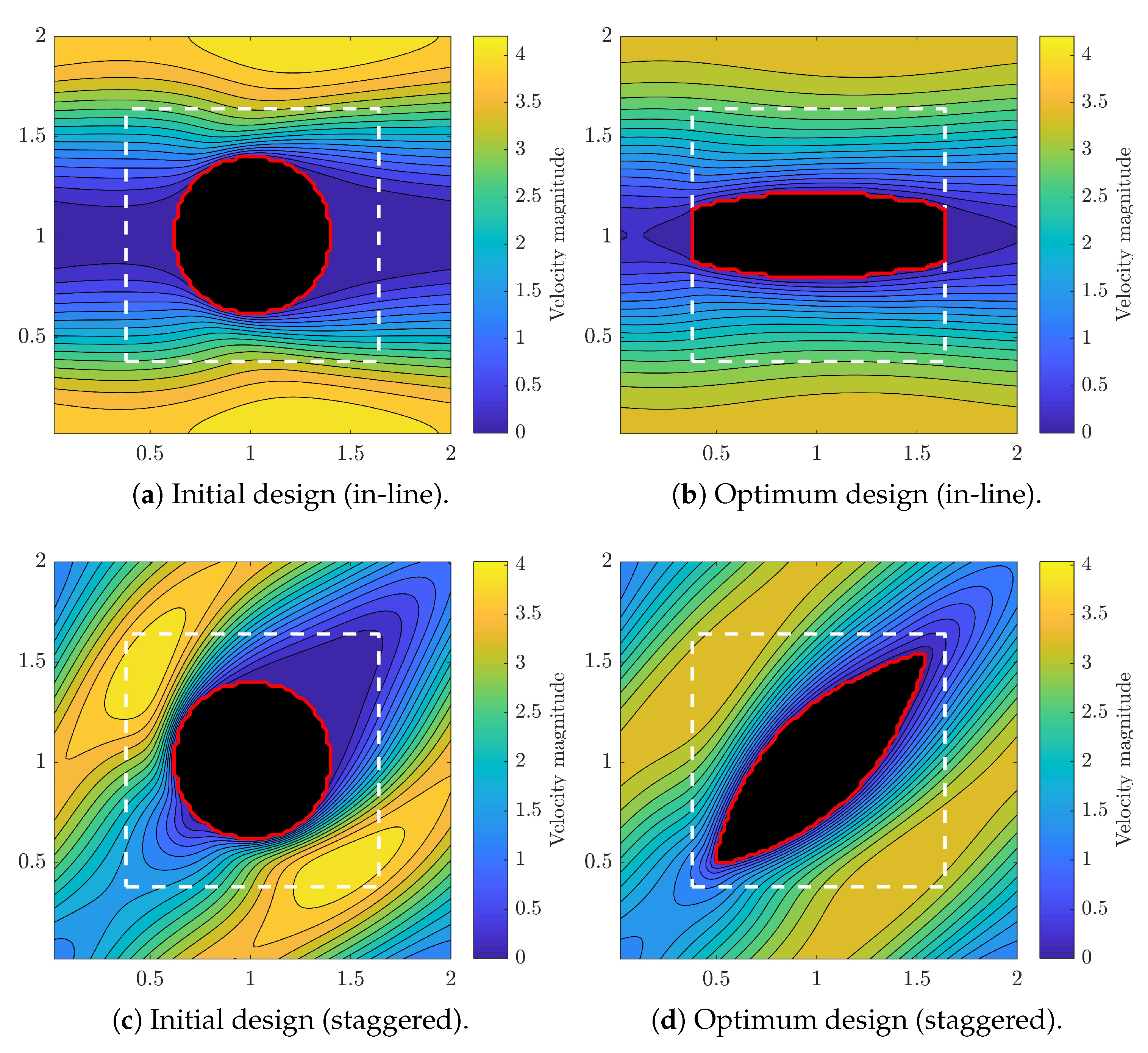
Figure 5 shows the initial and optimal fin topologies as well as the flow velocity field, for both in-line and staggered arrays at $Re=25$. For in-line array, as shown in Figure 5b, the optimum design is stretched stream-wise to increase the cross-section aspect-ratio and reduce the frontal area to for a more hydrodynamic fin. The upper and lower surface curvatures facilitate the flow from tip to tail, because the main flow stream has a periodic converging–diverging format. As the result, the optimal design features ∼39% less drag force, as listed in

Table 1. Initial and optimum drag coefficients ($C_D$) for case 1.

Test Problem: Case 1 (a)	Initial ${\mathit{C}}_{\mathit{D}}$	Final ${\mathit{C}}_{\mathit{D}}$	Drag Change	Initial Max. Gap Velocity	Final Max. Gap Velocity
(a) In-line	2.5717	1.5673	$-39.06\%$	4.29	4.12
(a) Staggered	4.3207	2.6159	$-39.45\%$	3.58	3.40

. The first reason is that the frontal area is now smaller than the initial circular fin and each fins. The second reason is that the increased gap space between fin rows reduces the maximum flow velocity, and consequently the exerted drag force. We should also note that the front and end of the optimal fins are attached to the the border of design domain. This is not surprising, since at $Re=25$ the viscous drag is less severe than the pressure drag, and theoretically we know that parallel plates produce minimum drag. Therefore we observe that by increasing $L_D$, the optimizer minimizes the pressure drag by increasing gap space between fin rows and filling the gap space between upstream and downstream fins, until the fins are fully attached and a uniform parallel channels are created.

In staggered alignment, as shown in Figure 5c, the flow is not unidirectional and the fluid velocity magnitude in front of the fins is not negligible, which results in higher fin drag force and total pressure drop in staggered alignment compared to in-line. The optimal staggered fin, as shown in Figure 5d, is a symmetric convex cross-section shape, with sharp fronts and tails and less frontal areas, similar to airfoils. The wake region behind the original cylindrical fin is almost eliminated after the optimization which demonstrates a better flow guidance within the fin array. The maximum flow velocity is also reduced considerably, because of the increased cross-gap space. The drag force in staggered fin array after the optimization is $39.45\%$ less, while the total cross-section area is equivalent to the initial fin array. Overall, we find the results to be consistent with the physics of flow across the fins and the performance of the TO well satisfactory.

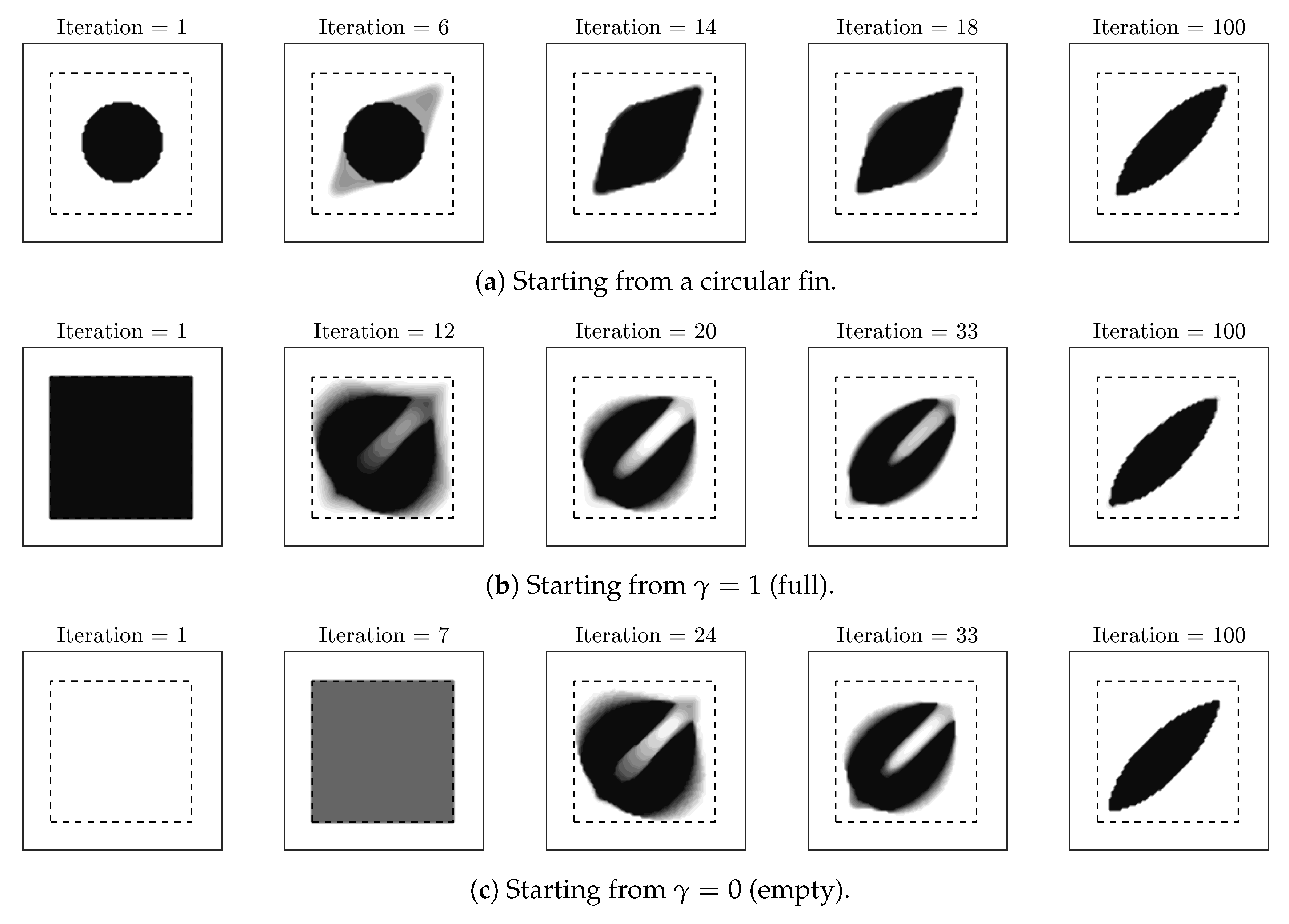
In case (b) of the first example, our goal is to investigate the robustness of our TO tool by examining different initial values for design variables and compare the final optimum topologies to verify whether the results are insensitive to the initial (unoptimized) designs. For this purpose, we repeat the previous topology optimization example of staggered configuration in case (a), but we set all the initial $\gamma$’s to either 1 (full solid) or 0 (no solid) and compare them with the initial circular fin. We note that the same volume constraint as the circular fin of case (a) is imposed; therefore, starting the optimization with no solid area violates the volume constraint in the beginning, however, we expect the optimizer to eventually satisfy that. 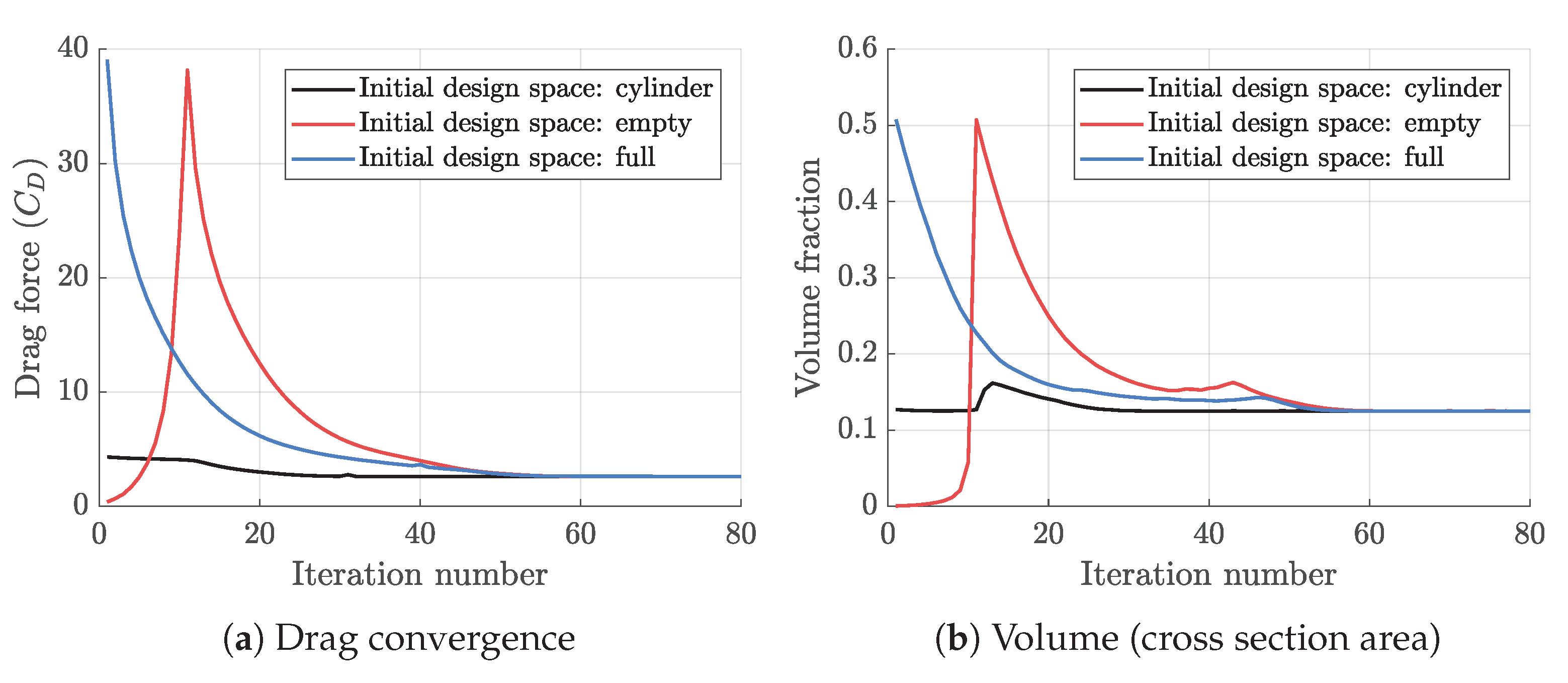Figure 6 illustrates the topology optimization process for those three different initial designs, and Figure 7 shows the convergence history of the drag forces, as well as the total fin volumes. We note that the optimization process for circular and full initial designs are rather smooth, because the optimization starts from feasible design space. On the other hand, for the case of empty initial design, the optimization process begins from infeasible state; therefore, the optimizer uniformly fills the design domain to first satisfy the minimum volume constraint (near to iteration 10), and then continues an optimization process similar to full solid case. Regardless of the starting phase, all three cases reached similar final topologies with closely identical drag forces. We also obtained similar performance for in-line configuration, and overall, we find the optimization processes promisingly insensitive to the initial design which confirm the robustness as we desired.

4.2. Case 2: Fin Geometry at Different Flow Reynolds Numbers

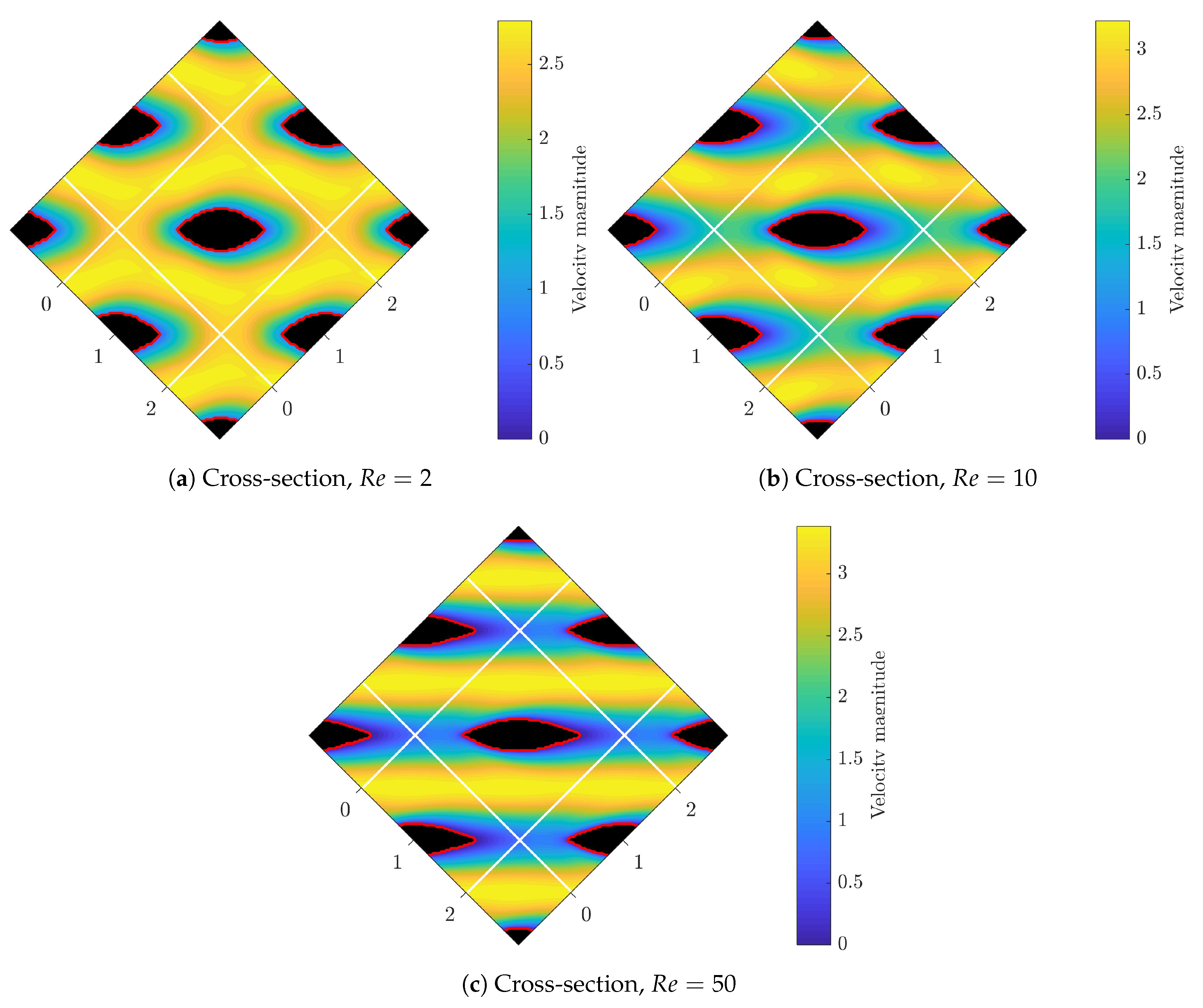
In this test example, we aim to investigate optimal fin topologies at different flow conditions, particularly at different Reynolds numbers. More precisely, the flow Reynolds number is the only variant in this study, and the rest of the parameters such as volume constraint are similar to the staggered case of 1-(a).

Figure 8 shows the schematic of optimized staggered fin arrays for Reynolds numbers of 2, 10 and 50, and in addition

Table 2. Final drag forces and aspect ratios for different Re numbers.

Reynolds Number	Drag Change (Reduction) (%)	Fin Aspect Ratio
2	−12.62%	1.99
5	−18.35%	2.39
10	−25.99%	2.68
25	−40.06%	3.22
50	−53.59%	3.63

also lists the fin aspect ratios as well as the optimal drag force compared to circular (unoptimized) fins. At first glance, we observe that optimizer has reduced the frontal areas and increased the spanwise length, to produce a better hydrodynamical shapes. At $Re=50$, drag force is $53.58\%$ reduced and fin cross-section shapes suggest the minimum frontal area as well as the maximum aspect ratio. In this case, the viscous drag is much less severe than the pressure drag, consequently fin has a relatively large aspect ratio of 3.63. On the other hand, at $Re=2$ flow is more viscus and therefore viscus drag is more dominant. In such case, fin shape has comparatively the least aspect ratio (1.99) with only $12.61\%$ reduced drag. As the flow Reynolds increases, the boundary layer becomes thiner and fins aspect ratios increases. The gap space between fins are larger and we observe a more straight flow stream which confirms a less dissipative flow. We note that for higher Reynolds numbers ($Re>100$), flow becomes unsteady and requires unsteady sensitivity analysis which is beyond the scope of this paper.

The promising fin array optimization results consistent with the flow conditions confirms the utility and flexibility of the present topology optimization approach to find the optimal geometries featuring the minimized pressure loss, as initially was targeted.

4.3. Case 3: Drag Minimization of Passive Designs

For the last example, we further consider to minimize drag (pressure loss) particularly for pre-designed circular arrays. More precisely, we keep the initial design unchanged during optimization such that the optimizer is allowed to merely add solid zones to the initial fins. In this regard, we decompose the design domain into two parts: passive domain, ${\mathsf{\Omega }}_D^p$, and active domain, ${\mathsf{\Omega }}_D^a$. In the passive domain corresponding to the initial fin design, $\gamma$’s are fixed to 1 during optimization, however, in the active domain, the design variables are free to change as before. In summary, we can define the two domains by

$$\left\{\begin{array}{cc}{\gamma }_i=1\hfill & \mathrm{if}{\gamma }_i\in {\mathsf{\Omega }}_D^p(\mathrm{only}\mathrm{solid})\hfill \\ 0\le {\gamma }_i\le 1\hfill & \mathrm{if}{\gamma }_i\in {\mathsf{\Omega }}_D^a(\mathrm{solid}\mathrm{or}\mathrm{fluid}),\hfill \end{array}\right.$$

(32)

where ${\mathsf{\Omega }}_D^p+{\mathsf{\Omega }}_D^a={\mathsf{\Omega }}_D$.

The main purpose of this example is to demonstrate the utility of our TO tool to minimize fin drag force, while the frontal projected area as well as the gap spaces can not be reduced anymore. We perform unconstrained optimization procedure, therefore, no volume constraint is imposed in this case, however, increasing solid volumes reduces the total empty space for fluid to flow, which may cause higher flow velocity and drag forces. For this task, we use again staggered cylindrical fin arrays with various sizes as the initial designs, at $Re=50$. 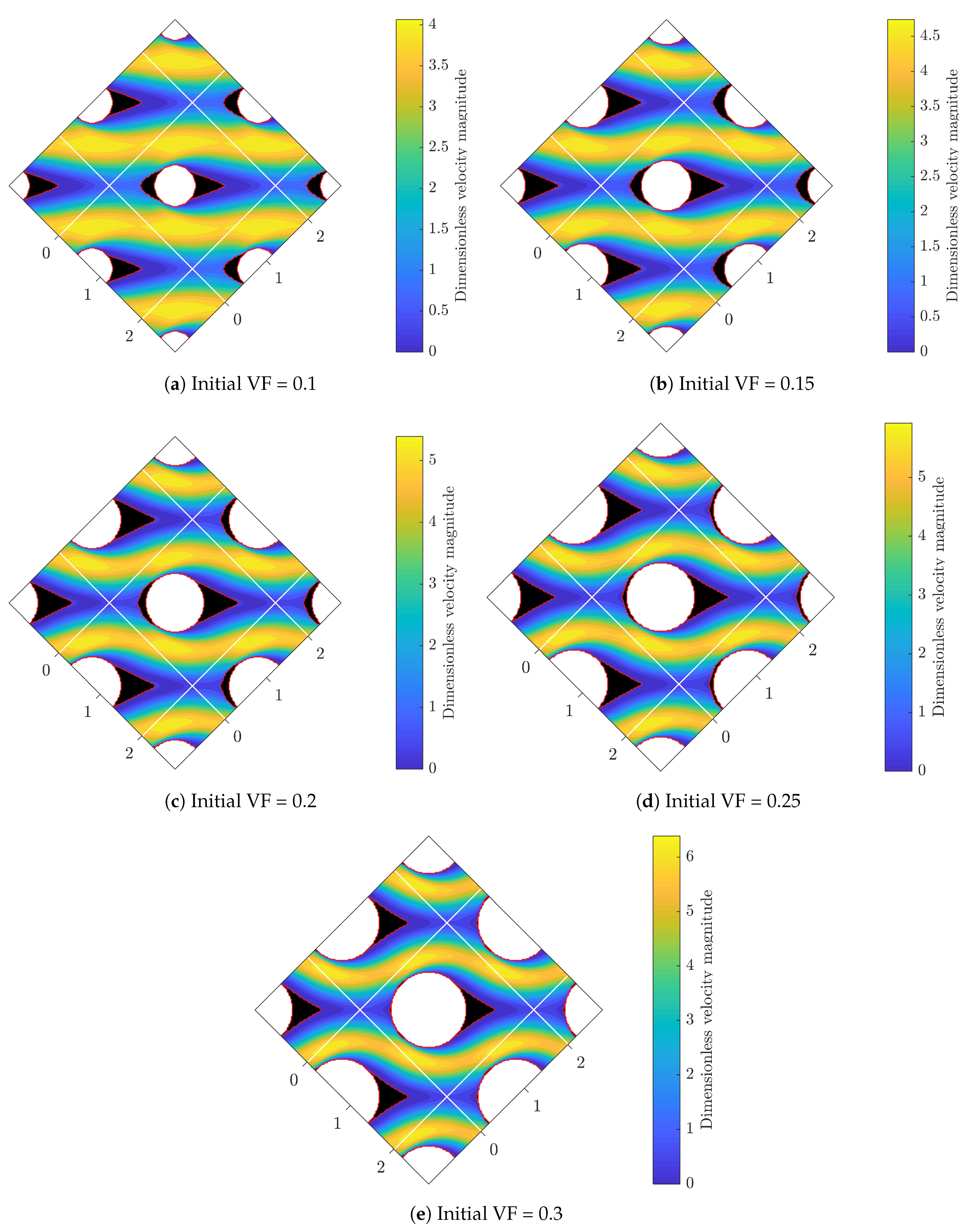Figure 9 shows the initial designs in white and the newly added parts after optimization in black. In all cases, after the optimization two solid parts are created and attached to the cylinders, one to the tip and one to the tail of the cylinders, in the streamwise direction The added parts facilitate fluid flow in front and in wake spaces to reduce high stagnation pressure and modify the low pressure wake region, respectively. As listed in

Table 3. Drag reduction of passive fin design by topology optimization.

Initial		Optimized
Solid Volume Fraction	${\mathbf{C}}_{\mathbf{D}}$	Solid Volume Fraction	${\mathbf{C}}_{\mathbf{D}}$	Drag Changes (%)
0.10	3.41	0.151	3.19	−6.54
0.15	4.32	0.216	3.95	−8.57
0.20	5.43	0.271	4.94	−9.02
0.25	6.45	0.310	5.97	−7.44
0.30	7.43	0.343	7.07	−4.85

, the optimal topologies with better hydrodynamical profiles promisingly produce up to 9% less drag forces, while the frontal projected areas remained fixed.

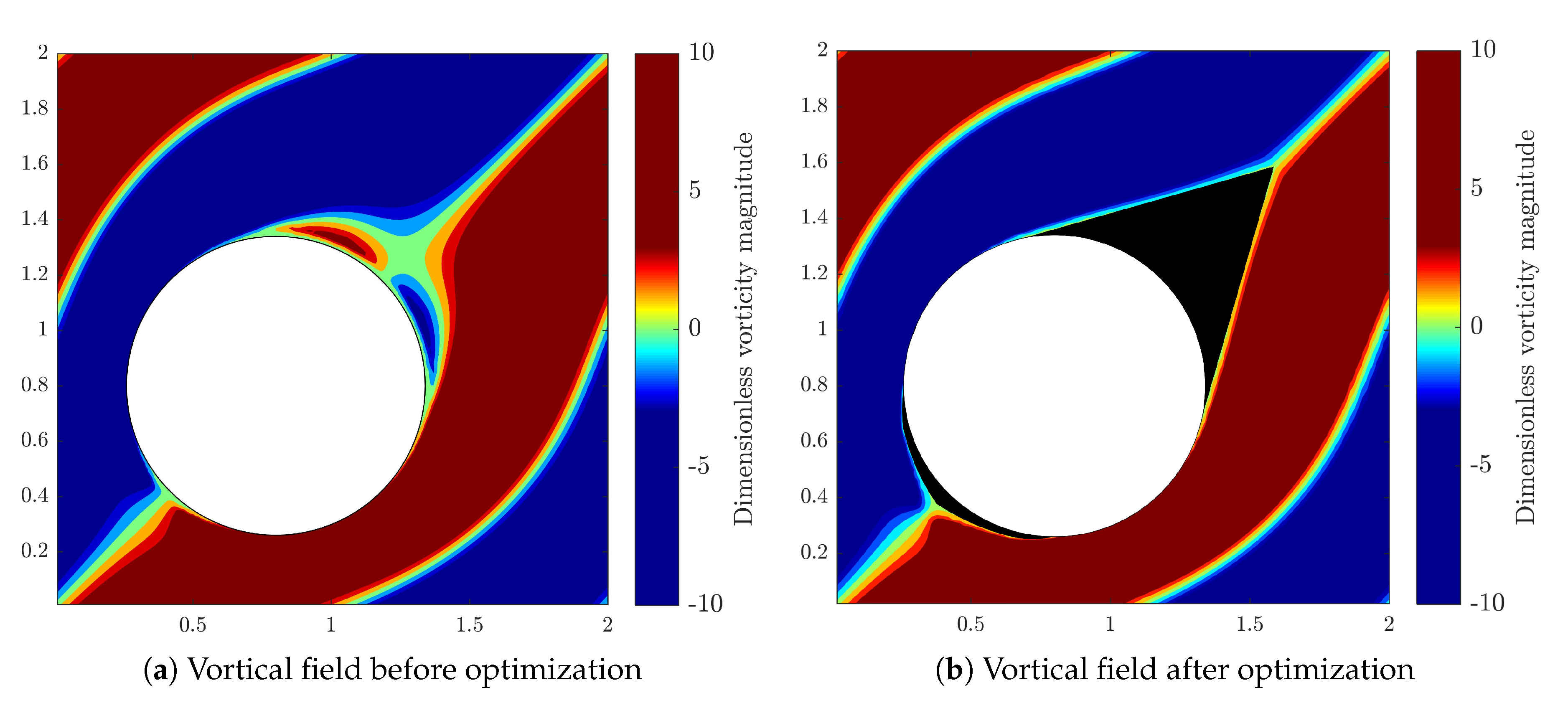
To better understand functionality and reveal the importance of an added tail, we examine the vorticity fields before and after the optimization. As plotted in Figure 10a, two vortices exist after the flow separation points in the wake region, behind the cylinders. The low pressurized wake area considerably contributes to the pressure drag and increases the total pressure loss. However, as shown in Figure 10b, the added tail in the optimal fin profile has properly filled the wake area. In the optimal design, flow experiences a very smooth path and back flow pressure is fully recovered. Flow separation has been successfully eliminated, which leads to a less energy dissipative flow regime. For smaller solid volume fractions, pitch distance and gap space are relatively large, therefore, the mainstream flow is roughly straight. In this case, the optimal fin shape resembles an airfoil with larger aspect ratio and longer tail to better guide the flow and and recover back pressure. On the other hand, for larger solid volume fractions, the flow path is wavy with high curvature. The maximum velocity, due to the smaller gap space, is also larger, and flow magnitude in the front and back of the fins is considerable. The added tip and tail elements conform to the wavy flow stream, nevertheless, they are relatively smaller. At highest volume fraction (VF = 0.3), the tip element almost vanishes but a tail is again added to better guide the flow in the wake and recover the pressure. We note that the optimizer has satisfyingly modified the circular fin arrays for all volume fractions and as promised, successfully minimized drag forces, nevertheless the frontal area was kept fixed.

5. Conclusions

We presented a novel topology optimization tool for hydrodynamic drag (power loss) minimization of fin arrays. We developed our numerical topology optimization approach based on the accurate and powerful pseudo-spectral scheme equipped with the Brinkman penalization method. We provided a detailed sensitivity analysis, derived directly from a pseudo-spectral scheme and chain rule of differentiation, and verified it by a finite differencing method. We also applied few techniques, such as a convenient algebraic factorization, to substantially increase computational efficiency and reduce total cost of optimization. Using several test examples, we investigated the accuracy, flexibility and robustness of our tool. We successfully reduced the drag force (pressure loss) of a circular fin array by up to ∼53.6%, and conveniently obtained optimal fin geometries at different Reynolds numbers (from 2 to 50), for both in-line and staggered arrays. We lastly performed several unconstrained topology optimization test cases to investigate the numerical flexibility in terms minimizing the drag for passive fin designs. Interestingly, the optimal topologies eliminated flow separation as well as low pressure wake by adding tip and tail, and reduced drag forces up to $9\%$, nevertheless, the frontal projected area was fixed.