Proportional Resonant Current Control and Output-Filter Design Optimization for Grid-Tied Inverters Using Grey Wolf Optimizer


Abstract
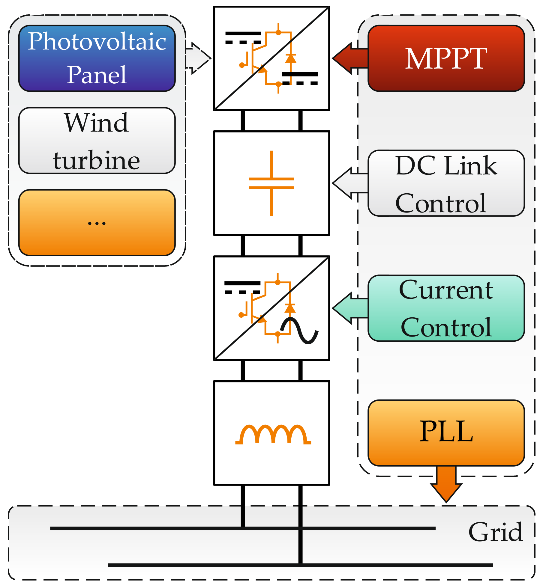
1. Introduction
2. Control Schemes
2.1. PR Current Controller
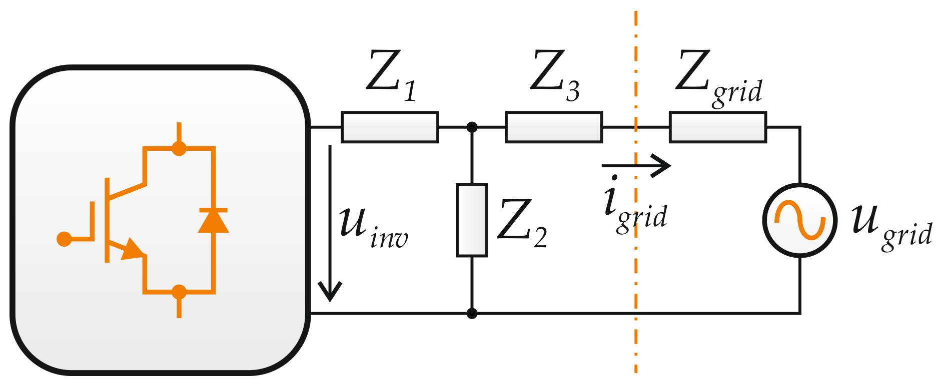
2.2. Output Filter Topologies
3. Optimization Procedure
Proposed Methodology
4. Simulation and Results
4.1. First Case Study—SPD Topology
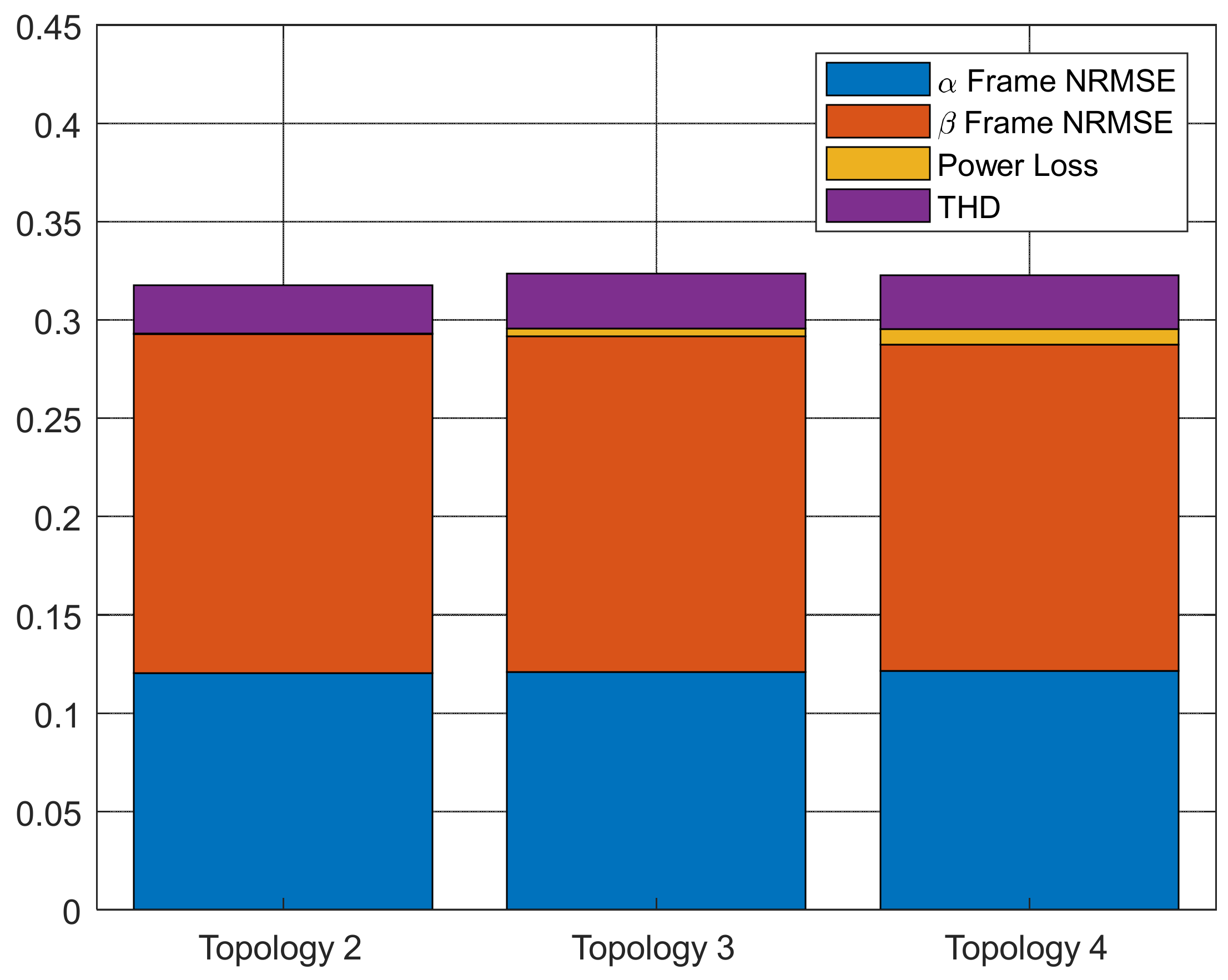
4.2. Second Case Study—CPD Topologies
5. Conclusions
Author Contributions
Funding
Conflicts of Interest
References
- Blaabjerg, F.; Yang, Y.; Yang, D.; Wang, X. Distributed Power-Generation Systems and Protection. Proc. IEEE 2017, 105, 1311–1331. [Google Scholar] [CrossRef]
- Faria, J.; Pombo, J.; Calado, M.; Mariano, S. Power Management Control Strategy Based on Artificial Neural Networks for Standalone PV Applications with a Hybrid Energy Storage System. Energies 2019, 12, 902. [Google Scholar] [CrossRef]
- Zakzouk, N.E.; Abdelsalam, A.K.; Helal, A.A.; Williams, B.W. High Performance Single-Phase Single-Stage Grid-Tied PV Current Source Inverter Using Cascaded Harmonic Compensators. Energies 2020, 13, 380. [Google Scholar] [CrossRef]
- Faria, J.; Pombo, J.; Calado, M.d.R.; Mariano, S. Current Control Optimization for Grid-Tied Inverters Using Cuckoo Search Algorithm. In Proceedings of the International Congress on Engineering University da Beira Interior—“Engineering for Evolution”, Covilhã, Portugal, 27–29 November 2019. [Google Scholar]
- Committee, D.; Power, I.; Society, E. IEEE Std 519-2014 (Revision of IEEE Std 519-1992); IEEE: Piscataway, NJ, USA, 2014; Volume 2014. [Google Scholar] [CrossRef]
- Dong, R.; Liu, S.; Liang, G. Research on Control Parameters for Voltage Source Inverter Output Controllers of Micro-Grids Based on the Fruit Fly Optimization Algorithm. Appl. Sci. 2019, 9, 1327. [Google Scholar] [CrossRef]
- Husev, O.; Roncero-Clemente, C.; Makovenko, E.; Pimentel, S.P.; Vinnikov, D.; Martins, J. Optimization and Implementation of the Proportional-Resonant Controller for Grid-Connected Inverter with Significant Computation Delay. IEEE Trans. Ind. Electron. 2020, 67, 1201–1211. [Google Scholar] [CrossRef]
- Singh, J.K.; Behera, R.K. Hysteresis Current Controllers for Grid Connected Inverter: Review and Experimental Implementation. In Proceedings of the IEEE International Conference on Power Electronics, Drives and Energy Systems, PEDES 2018, Chennai, India, 18–21 December 2018; Institute of Electrical and Electronics Engineers Inc.: Piscataway, NJ, USA, 2018. [Google Scholar] [CrossRef]
- Pouresmaeil, E.; Akorede, M.F.; Montesinos-Miracle, D.; Gomis-Bellmunt, O.; Trujillo Caballero, J.C. Hysteresis Current Control Technique of VSI for Compensation of Grid-Connected Unbalanced Loads. Electr. Eng. 2014, 96, 27–35. [Google Scholar] [CrossRef]
- Qazi, S.H.; Mustafa, M.W.; Ali, S. Review on Current Control Techniques of Grid Connected PWM-VSI Based Distributed Generation. Trans. Electr. Eng. Electron. Commun. 2019, 17, 152–168. [Google Scholar] [CrossRef]
- Bielskis, E.; Baskys, A.; Valiulis, G. Controller for the Grid-Connected Microinverter Output Current Tracking. Symmetry 2020, 12, 112. [Google Scholar] [CrossRef]
- Kojabadi, H.M.; Yu, B.; Gadoura, I.A.; Chang, L.; Ghribi, M. A Novel DSP-Based Current-Controlled PWM Strategy for Single Phase Grid Connected Inverters. IEEE Trans. Power Electron. 2006, 21, 985–993. [Google Scholar] [CrossRef]
- Moghaddam, A.F.; Van Den Bossche, A. Investigation of a Delay Compensated Deadbeat Current Controller for Inverters by Z-Transform. Electr. Eng. 2018, 100, 2341–2349. [Google Scholar] [CrossRef]
- Naderipour, A.; Asuhaimi, A.; Zin, M.; Hafiz, M.; Habibuddin, B.; Miveh, M.R.; Guerrero, J.M.; Asuhaimi Mohd Zin, A.; Bin Habibuddin, M.H.; Miveh, M.R.; et al. An Improved Synchronous Reference Frame Current Control Strategy for a Photovoltaic Grid-Connected Inverter under Unbalanced and Nonlinear Load Conditions. PLoS ONE 2017, 12. [Google Scholar] [CrossRef] [PubMed]
- Meral, M.E.; Çelik, D. Comparison of SRF/PI- and STRF/PR-Based Power Controllers for Grid-Tied Distributed Generation Systems. Electr. Eng. 2018, 100, 633–643. [Google Scholar] [CrossRef]
- Golestan, S.; Ebrahimzadeh, E.; Guerrero, J.M.; Vasquez, J.C. An Adaptive Resonant Regulator for Single-Phase Grid-Tied VSCs. IEEE Trans. Power Electron. 2018, 33, 1867–1873. [Google Scholar] [CrossRef]
- Yazdani, A.; Iravani, R. Voltage-Sourced Converters in Power Systems: Modeling, Control, and Applications; IEEE Press: Piscataway, NJ, USA; John Wiley: Hoboken, NJ, USA, 2010. [Google Scholar]
- Kalaam, R.N.; Muyeen, S.M.; Al-Durra, A.; Hasanien, H.M.; Al-Wahedi, K. Optimisation of Controller Parameters for Gridtied Photovoltaic System at Faulty Network Using Artificial Neural Network-Based Cuckoo Search Algorithm. IET Renew. Power Gener. 2017, 11, 1517–1526. [Google Scholar] [CrossRef]
- Qais, M.H.; Hasanien, H.M.; Alghuwainem, S. A Grey Wolf Optimizer for Optimum Parameters of Multiple PI Controllers of a Grid-Connected PMSG Driven by Variable Speed Wind Turbine. IEEE Access 2018, 6, 44120–44128. [Google Scholar] [CrossRef]
- Guha, D.; Roy, P.K.; Banerjee, S. Grasshopper Optimization Algorithm-Scaled Fractional-Order PI-D Controller Applied to Reduced-Order Model of Load Frequency Control System. Int. J. Model. Simul. 2019, 1–26. [Google Scholar] [CrossRef]
- Dash, P.; Saikia, L.C.; Sinha, N. Automatic Generation Control of Multi Area Thermal System Using Bat Algorithm Optimized PD-PID Cascade Controller. Int. J. Electr. Power Energy Syst. 2015, 68, 364–372. [Google Scholar] [CrossRef]
- Qi, Z.; Shi, Q.; Zhang, H. Tuning of Digital PID Controllers Using Particle Swarm Optimization Algorithm for a CAN-Based DC Motor Subject to Stochastic Delays. IEEE Trans. Ind. Electron. 2019, 67, 5637–5646. [Google Scholar] [CrossRef]
- Khan, I.A.; Alghamdi, A.S.; Jumani, T.A.; Alamgir, A.; Awan, A.B.; Khidrani, A. Salp Swarm Optimization Algorithm-Based Fractional Order PID Controller for Dynamic Response and Stability Enhancement of an Automatic Voltage Regulator System. Electronics 2019, 8, 1472. [Google Scholar] [CrossRef]
- Patel, N.C.; Debnath, M.K. Whale Optimization Algorithm Tuned Fuzzy Integrated PI Controller for LFC Problem in Thermal-Hydro-Wind Interconnected System. In Lecture Notes in Electrical Engineering; Springer: Berlin, Germany, 2019; Volume 553, pp. 67–77. [Google Scholar] [CrossRef]
- Huang, M.; Li, H.; Wu, W.; Blaabjerg, F. Observer-Based Sliding Mode Control to Improve Stability of Three-Phase LCL-Filtered Grid-Connected VSIs. Energies 2019, 12, 1421. [Google Scholar] [CrossRef]
- Beres, R.N.; Wang, X.; Liserre, M.; Blaabjerg, F.; Bak, C.L. A Review of Passive Power Filters for Three-Phase Grid-Connected Voltage-Source Converters. IEEE J. Emerg. Sel. Top. Power Electron. 2016, 4, 54–69. [Google Scholar] [CrossRef]
- Gomes, C.C.; Cupertino, A.F.; Pereira, H.A. Damping Techniques for Grid-Connected Voltage Source Converters Based on LCL Filter: An Overview. Renew. Sustain. Energy Rev. 2018, 81, 116–135. [Google Scholar] [CrossRef]
- Huang, M.; Blaabjerg, F.; Loh, P.C. The Overview of Damping Methods for Three-Phase Grid-Tied Inverter with LLCL-Filter. In Proceedings of the 16th European Conference on Power Electronics and Applications, Lappeenranta, Finland, 26–28 August 2014. [Google Scholar] [CrossRef]
- Peña-Alzola, R.; Blaabjerg, F. Design and Control of Voltage Source Converters with LCL-Filters. In Control of Power Electronic Converters and Systems; Elsevier: Amsterdam, The Netherlands, 2018; pp. 207–242. [Google Scholar] [CrossRef]
- Jalili, K.; Bernet, S. Design of LCL Filters of Active-Front-End Two-Level Voltage-Source Converters. IEEE Trans. Ind. Electron. 2009, 56, 1674–1689. [Google Scholar] [CrossRef]
- Channegowda, P.; John, V. Filter Optimization for Grid Interactive Voltage Source Inverters. IEEE Trans. Ind. Electron. 2010, 57, 4106–4114. [Google Scholar] [CrossRef]
- Kim, Y.-J.; Kim, H. Optimal Design of LCL Filter in Grid-Connected Inverters. IET Power Electron. 2019, 12, 1774–1782. [Google Scholar] [CrossRef]
- Zhang, D.; Dutta, R. Application of Partial Direct-Pole-Placement and Differential Evolution Algorithm to Optimize Controller and LCL Filter Design for Grid-Tied Inverter. In Proceedings of the Australasian Universities Power Engineering Conference, AUPEC 2014, Perth, WA, Australia, 28 September–1 October 2014; pp. 1–6. [Google Scholar] [CrossRef]
- Jianfeng, L.; Meiyu, L.; Guangzheng, Y.; Rusi, C. Parameter Optimization Design Method of LCL Filter Based on Harmonic Stability of VSC System. In Proceedings of the 4th International Conference on Intelligent Green Building and Smart Grid, IGBSG 2019, Yi-chang, China, 6–9 September 2019; pp. 226–231. [Google Scholar] [CrossRef]
- Chatterjee, A.; Mohanty, K.B. Current Control Strategies for Single Phase Grid Integrated Inverters for Photovoltaic Applications—A Review. Renew. Sustain. Energy Rev. 2018, 92, 554–569. [Google Scholar] [CrossRef]
- Liang, W.; Liu, Y.; Ge, B.; Wang, X. DC-Link Voltage Balance Control Strategy Based on Multidimensional Modulation Technique for Quasi-Z-Source Cascaded Multilevel Inverter Photovoltaic Power System. IEEE Trans. Ind. Inform. 2018, 14, 4905–4915. [Google Scholar] [CrossRef]
- Zou, Z.-X.; Rosso, R.; Liserre, M. Modeling of the Phase Detector of a Synchronous-Reference-Frame Phase-Locked Loop Based on Second-Order Approximation. IEEE J. Emerg. Sel. Top. Power Electron. 2019. [Google Scholar] [CrossRef]
- Teodorescu, R.; Liserre, M.; Rodriguez, P. Grid Converters for Photovoltaic and Wind Power Systems; John Wiley & Sons, Ltd.: Hoboken, NJ, USA, 2011. [Google Scholar] [CrossRef]
- Teodorescu, R.; Blaabjerg, F.; Liserre, M.; Loh, P.C. Proportional-Resonant Controllers and Filters for Grid-Connected Voltage-Source Converters. IEE Proc. Electr. Power Appl. 2006, 153, 750. [Google Scholar] [CrossRef]
- Wu, W.; He, Y.; Tang, T.; Blaabjerg, F. A New Design Method for the Passive Damped LCL and LLCL Filter-Based Single-Phase Grid-Tied Inverter. IEEE Trans. Ind. Electron. 2013, 60, 4339–4350. [Google Scholar] [CrossRef]
- Mirjalili, S.M.; Mirjalili, S.M.; Lewis, A. Grey Wolf Optimizer. Adv. Eng. Softw. 2014, 69, 46–61. [Google Scholar] [CrossRef]
- Reznik, A.; Simoes, M.G.; Al-Durra, A.; Muyeen, S.M. LCL Filter Design and Performance Analysis for Grid-Interconnected Systems. IEEE Trans. Ind. Appl. 2014, 50, 1225–1232. [Google Scholar] [CrossRef]


| Parameters | Topology 1 | Topology 2 | Topology 3 | Topology 4 | ||||
|---|---|---|---|---|---|---|---|---|
| Lower Bound | Upper Bound | Lower Bound | Upper Bound | Lower Bound | Upper Bound | Lower Bound | Upper Bound | |
| L1 (mH) | 0.01 | 4 | 0.01 | 4 | 0.01 | 4 | 0.01 | 4 |
| L2 (mH) | 0.01 | 4 | 0.01 | 4 | 0.01 | 4 | 0.01 | 4 |
| Ld (mH) | 0.01 | 4 | 0.01 | 4 | ||||
| C (μF) | 1 × 10⁻⁵ | 10 | 1 × 10⁻⁵ | 10 | 1 × 10⁻⁵ | 10 | 1 × 10⁻⁵ | 10 |
| Cd (μF) | 1 × 10⁻⁵ | 2.5 | 1 × 10⁻⁵ | 0.5 | ||||
| Rd (Ω) | 0.5 | 200 | 0.5 | 200 | 0.5 | 200 | 0.5 | 200 |
| kp | 100 | 600 | 100 | 600 | 100 | 600 | 100 | 600 |
| kr | 1 × 10³ | 25 × 104 | 1 × 10³ | 25 × 104 | 1 × 10³ | 25 × 104 | 1 × 10³ | 25 × 104 |
| Parameters | L1 (mH) | L2 (mH) | C (μF) | Rd (Ω) | kr | kp | fobj |
|---|---|---|---|---|---|---|---|
| Topology SPD | 4 | 0.723 | 0.868 | 4.63 | 86,245.556 | 180.198 | 0.3210 |
| Parameters | L1 (mH) | L2 (mH) | Ld (mH) | C (μF) | Cd (μF) | Rd (Ω) | kr | kp | fobj |
|---|---|---|---|---|---|---|---|---|---|
| Topology 2 | 3.7 | 0.135 | 4.71 | 1.68 | 2.42 | 78,945.05 | 173.13 | 0.317 | |
| Topology 3 | 3.8 | 0.729 | 0.41 | 6.08 | 82.3 | 93,109.50 | 199.24 | 0.323 | |
| Topology 4 | 3.78 | 2.44 | 2.91 | 3.86 | 2.72 | 172.73 | 129,451.34 | 287.27 | 0.322 |
© 2020 by the authors. Licensee MDPI, Basel, Switzerland. This article is an open access article distributed under the terms and conditions of the Creative Commons Attribution (CC BY) license (http://creativecommons.org/licenses/by/4.0/).
Share and Cite
Faria, J.; Fermeiro, J.; Pombo, J.; Calado, M.; Mariano, S. Proportional Resonant Current Control and Output-Filter Design Optimization for Grid-Tied Inverters Using Grey Wolf Optimizer. Energies 2020, 13, 1923. https://doi.org/10.3390/en13081923
Faria J, Fermeiro J, Pombo J, Calado M, Mariano S. Proportional Resonant Current Control and Output-Filter Design Optimization for Grid-Tied Inverters Using Grey Wolf Optimizer. Energies. 2020; 13(8):1923. https://doi.org/10.3390/en13081923
Chicago/Turabian StyleFaria, João, João Fermeiro, José Pombo, Maria Calado, and Sílvio Mariano. 2020. "Proportional Resonant Current Control and Output-Filter Design Optimization for Grid-Tied Inverters Using Grey Wolf Optimizer" Energies 13, no. 8: 1923. https://doi.org/10.3390/en13081923
APA StyleFaria, J., Fermeiro, J., Pombo, J., Calado, M., & Mariano, S. (2020). Proportional Resonant Current Control and Output-Filter Design Optimization for Grid-Tied Inverters Using Grey Wolf Optimizer. Energies, 13(8), 1923. https://doi.org/10.3390/en13081923