Lifetime Analysis of IGBT Power Modules in Passively Cooled Tidal Turbine Converters

Abstract

Thermal cycling is one of the major reasons for failure in power electronic converters. For submerged tidal turbine converters investigating this failure mode is critical in improving the reliability, and minimizing the cost of energy from tidal turbines. This paper considers a submerged tidal turbine converter which is passively cooled by seawater, and where the turbine has fixed-pitch blades. In this respect, this study is different from similar studies on wind turbine converters, which are mostly cooled by active methods, and where turbines are mostly pitch controlled. The main goal is to quantify the impact of surface waves and turbulence in tidal stream velocity on the lifetime of the converter IGBT (insulated gate bipolar transistor) modules. The lifetime model of the IGBT modules is based on the accumulation of fatigue due to thermal cycling. Results indicate that turbulence and surface waves can have a significant impact on the lifetime of the IGBT modules. Furthermore, to accelerate the speed of the lifetime calculation, this paper uses a modified approach by dividing the thermal models into low and high frequency models. The final calculated lifetime values suggest that relying on passive cooling could be adequate for the tidal converters as far as thermal cycling is concerned.

1. Introduction

Power electronic converters in tidal turbine drive trains regulate the power capture from the turbine, and convert the generated electricity into a grid compliant form at fixed voltage and frequency. The converter can be placed either onshore, on floating platforms, or they can be seabed-mounted adjacent to the generator. In this paper we consider the seabed-mounted converter as shown in Figure 1. This configuration is more suitable for array applications as it minimizes cabling costs [1], involves no hanging cables, and is out of view. However, submerged power converter also means limited access for maintenance, and hence reliability is paramount [1]. Improving reliability, and thus capacity factor, could be a major contributor to lowering the levelized cost of energy (LCoE) from tidal turbines [2]. According to Reference [1], subsea converters for tidal farms will demand more than 5-year mean period between failures.

Due to similar operating principle, it is reasonable to assume that many modes of failures in tidal turbines would be similar to wind turbines (WTs). However, the frequency of occurrences of these expected failure modes may differ in each case. Multiple studies have identified converters as one of the most frequently failing subsystem in WTs [3,4]. Among converter components, phase modules (insulated gate bipolar transistors (IGBTs), gate-drive circuits, capacitors) were found to be more critical in terms of failure frequency [3,5,6].

Thermal cycling has been identified as one of the main reasons for failure in IGBT power modules [3,7,8,9,10]. Early failures from thermal cycling stresses can be prevented by cooling power modules [3,9,10]. This cooling can be provided either by active methods such as forced-water cooling, or by passive cooling. By passive cooling we mean a system where no active devices such as pumps or fans and so forth. are used to cool the power modules. A simple possible example is to use a sealed enclosure inside which the power electronics module is bolted/welded to its walls, as shown in Figure 2 [11,12]. In this case the heat is conducted from the power module base plate to the walls of the enclosure and finally dumped in the ambient seawater by natural convection.

The main objective of this paper is to analyze whether passive cooling is a feasible option for a subsea converter from the reliability viewpoint. The reliability analysis is based on estimating the lifetime of the IGBT power modules in a tidal turbine converter, considering thermal cycling as the main failure mode. In this regard, the effect of turbulence in the tidal stream velocity and surface waves on the converter lifetime is analyzed.

Liu et al. [13] consider the reliability of the power converter in a doubly-fed induction generator based tidal turbine. They show the impact of probability distribution of tidal velocity on the converter reliability. Ren et al. [14] use a sequential Monte-Carlo simulation-based method to quantify effects of wake on tidal generator systems reliability in a tidal current farm. However, these studies do not specifically target the lifetime damage from thermal cycling in power converters, nor do they incorporate effects of turbulence or surface waves on the converter lifetime.

Extensive research has been carried out to study the lifetime models of power modules based on thermal cycling [15,16,17,18]. Nowadays, a priori estimation of lifetime is considered a logical step in designing reliable power electronic systems [9,19,20].

Shipurkar et al. [6] compared different 3-level converter topologies for WT converters based on thermal lifetime models. Reliability of WT converters ranging from the influence of mission profiles to that of reactive power on the lifetime of IGBT modules, and comparison of multilevel converter topologies, and so forth [19,21,22,23] is also widely studied. Active control of cooling systems, switching frequency and modulation strategies, and power loss redistribution (in case of parallel converters) are some commonly used techniques to improve lifetime in WT converters [24,25,26]. Adding redundancy is another way of improving the overall reliability in WT converters and subsea applications [1,27].

Most of the aforementioned WT lifetime studies cover mutli-MW pitch controlled turbines with 3-level medium voltage drives cooled by active methods (either water or air-cooled). This is the most common topology in modern WTs. However, active cooling mechanism usually suffer from drawbacks such as pump failure and leakage of the coolant, and so forth, which compromises the reliability to a certain degree.

The power converter under study in this paper is different from a WT converter for the following reasons. Firstly, this study considers a passively cooled submerged converter to minimize potential fault points. For tidal turbines with submerged converter, an active cooling method is unsuitable due to high maintenance costs, and limited opportunities for maintenance. Secondly, modern WTs usually employ pitch control, which makes the converter design different from a tidal turbine converter with active speed stall control investigated here. Thirdly, effects of site parameters, such as turbulence and waves on sea surface, is likely to have more impact on tidal turbine converters than on WT converters because of the higher speed oscillations in smaller scale tidal turbines. Finally, an exhaustive lifetime analysis on the tidal turbines is missing in the literature.

Thermal cycling is not the only failure mechanism in IGBT modules. Fischer et al. [5] identified ambient humidity and moisture as the dominant failure mechanism in WT converters. However, in their study majority of the converters were liquid-cooled. On the other hand, hermetically sealed converters are less likely to fail due to moisture, which is the case with subsea power converters analysed in this study. Other failure mechanisms include corrosion, dielectric breakdown, and so forth [27]. These failure mechanisms, however are extraneous to this study. For deep subsea applications (>100 m) power converters are enclosed in pressurized enclosures [28,29]. However, tidal turbines are rarely deployed at this depth, hence, we do not consider pressurized power converters in this study.

The IGBT power packs considered in this study are packed in the form of power modules rather than discs. Despite low potential for cooling, modules are preferred because of better assembly, integrated packaging, and good electrical isolation between the chip and the heat sink, and most importantly low cost compared to other packaging methods [30].

The main contributions from this paper, therefore, are:

–

To assess the effect of turbulence and surface waves on the lifetime of semiconductor components for a passively cooled power converter coupled to a tidal turbine;

–

To demonstrate the effect of active speed stall control and lower inertia of tidal turbines on the generator side converter lifetime; and to propose a methodology for faster lifetime calculation in a passively cooled converter.

To the best of our knowledge, these factors are for the first time being addressed in the literature.

The following section defines the parameters adopted for characterizing the site conditions of a typical tidal site. In Section 3, the description of the tidal turbine energy conversion system used for analysis is given. Section 4 describes the methodology adopted for the calculation of lifetime in passively cooled power converter. Section 5 briefly explains the thermal model of a seawater based passive cooling system. Section 6 gives the results of a case study carried on a 110 kW tidal turbine system. Conclusions from the paper are given in Section 7.

2. Site Conditions

For a submerged power converter, the thermal loading on the power module is determined by the ambient sea conditions, and the design of the power take-off (PTO) system. In this section, we look at the parameters used to characterize a typical tidal site for this study. The values presented here are later used for analysis in Section 6.

2.1. Mean Tidal Velocity

A tidal site with the frequency of occurrence as a function of tidal stream velocity is shown in Figure 3. This distribution profile is similar to that of the European Marine Energy Centre test facility in Orkney, Scotland [31].

Depending upon the location, a site may experience two flood and ebb tides roughly every 25 hours. Besides, most tidal sites also experience spring and neap tides roughly every 14 days, as shown in Figure 4. This information is relevant to investigate if the history of tidal velocity is also important for lifetime calculations, in addition to the instantaneous values.

2.2. Turbulence in the Tidal Stream Velocity

The instantaneous value of the tidal velocity differs from the mean tidal stream velocity. Figure 5 shows typical oscillations of the tidal velocity about its mean value. Some of these oscillations are attributed to the turbulence, usually characterized by the turbulence intensity values at the site. The turbulence intensity value is defined as [32],

$$TI=\frac{u^{\prime }}{\overline{u}},$$

(1)

where, $u^{\prime }$ and $\overline{u}$ denote the rms value of the velocity fluctuations and mean velocity respectively.

Multiple factors are responsible for turbulence, and accurate prediction of turbulence is too complex task to be undertaken in this analysis. Therefore in this paper, we use a stochastic flow field simulator called Turbsim to generate a more realistic tidal stream flow data. For tidal flows, Turbsim uses a modified version of the SMOOTH spectral model based on turbulent kinetic energy and shear. The tool has been developed at National Renewable Energy Laboratories, US [33].

Typically turbulence values differ with mean tidal velocity and vertical position of the turbine with respect to the seabed. Also, different turbulence intensity (TI) is expected for flood and ebb tides [32]. For the tidal site under consideration, TI values used are listed in

Table 1. Turbulence intensity values used to generate time series of tidal stream velocity.

Mean Velocity Range (m/s)	Mean TI Values (%)
Ebb tide
0.5 ≤ $\overline{u}$ ≤ 1.1	13.9
1.3 ≤ $\overline{u}$ ≤ 3.5	11.7
Flood tide
0.5 ≤ $\overline{u}$ ≤ 1.1	14.5
1.3 ≤ $\overline{u}$ ≤ 3.5	12.0

. Instead of using different TI for each mean tidal velocity, we have divided them into two main categories, in accordance with Reference [32].

2.3. Effect of Surface Waves

Waves on the sea surface may also cause oscillations in the velocity at the rotor hub. Zhou et al., studied the impact of these wave induced oscillations on the speed control of the tidal turbines [34]. The fluctuations about the mean tidal stream velocity at the rotor hub due to surface waves are calculated independently assuming the linear wave theory from the following equation [34]:

$$\Delta u\left(t\right)=\sum _i\frac{2\pi a_i}{T_i}\frac{cosh\left(2\pi \frac{z+d}{L_i}\right)}{sinh\left(2\pi \frac{z+d}{L_i}\right)}cos2\pi (\frac{t}{T_i}-\frac{x}{L_i}+{\varphi }_i),$$

(2)

where, $a_i$, $L_i$ and $T_i$ denote the amplitude, length and the period of the wave component respectively. z is the depth of the rotor hub, and d is the depth of the sea from the surface. The necessary parameters are listed in

Table 2. Turbine Rotor Parameters.

Parameter	Value
Hub depth from surface	20 m
Rotor Diameter	6.5 m
Seabed depth from surface	30 m

. In this paper, JONSWAP spectrum is chosen as the wave spectrum for not fully developed waves [35]. In other words, wave spectra is more dependent on local winds rather than the swell phenomenon [36]. Peak enhancement factor value for the spectrum is chosen as 3.3, which is the mean value for North Sea [37]. In Figure 5 the effect of turbulence (TI of 13%) and a surface wave (significant wave height, Hs = 5.75 m, and peak period, Tp = 11 s) on the mean tidal velocity (3.3 m/s) is shown. The extreme wave case is chosen here to make the effects of waves more visible.

A tidal site experiences different wave conditions throughout the year, and quantifying the impact of each wave condition on the lifetime of the IGBTs is a cumbersome task. Therefore, we limit ourselves to only analysing the impact of a representative summer and a winter month. We further assume that 6 such summer and winter months occur in a year. The total impact from all the waves in a year is calculated by estimating the impact from each wave condition, and then multiplying it with its probability of occurence. Probability density matrices for a representative summer and a winter month matrices are shown in

Table 3. Probability density (%) of waves according to significant wave heights and time periods for May 2009 at Orkney.

Tp(s), Hs(m)	0.25	0.75	1.25	1.75	2.25	2.75	3.25	3.75	4.25	4.75	5.25	5.75	6.25
3	6.92	2.82	2.35	0	0	0	0	0	0	0	0	0	0
5	4.97	0.27	0.87	0.47	0	0	0	0	0	0	0	0	0
7	3.96	0	0.07	1.75	1.01	0	0.74	0	0	0	0	0	0
9	5.98	0	1.81	0.34	0.2	0	0.94	0.87	0.40	0	0	0	0
11	2.48	3.76	4.77	6.72	6.18	3.96	2.08	0.07	1.61	0.27	0.27	0.13	0
13	0.47	1.07	2.89	4.91	2.22	2.01	4.57	4.30	0.27	0	0	0.13	0.20
15	0.47	0.67	0.13	0.34	0	0.20	0.13	2.55	0.87	0.40	0.20	0.34	0
17	0	0	0	0	0	0	0.13	0.26	1.14	0	0	0	0

and

Table 4. Probability density (%) of waves according to significant wave heights and time periods for November 2009 at Orkney.

Tp(s), Hs(m)	0.25	0.75	1.25	1.75	2.25	2.75	3.25	3.75	4.25	4.75	5.25	5.75	6.25
3	0	0.27	2.22	0	0	0	0	0	0	0	0	0	0
5	0	0.69	6.11	1.04	1.32	0.07	0	0	0	0	0	0	0
7	0	0	0.55	1.25	1.87	3.61	2.22	0.42	0	0	0	0	0
9	0	0	0.83	0	0.35	0.76	1.53	1.11	0	0	0	0	0
11	0	2.64	3.40	7.22	7.29	0.35	0	0	0	0	0	0	0
13	0	2.15	2.29	4.30	13.95	10.07	2.78	0.69	0	0	0	0	0
15	0	0	1.46	0.63	1.18	7.5	1.87	1.39	0	0	0	0	0
17	0	0	0.21	0	0	0.35	2.01	0	0	0	0	0	0

[38].

Again, the idea behind including fluctuations in tidal stream velocity in this study, whether due to turbulence or waves, is to investigate whether they will influence the lifetime of the IGBT modules.

2.4. Sea Temperature

The junction temperature of the IGBT also depends on the ambient temperature. In case of passive cooling, the ambient temperature also affects the external heat transfer coefficient, and thus the enclosure wall to ambient thermal resistance. For the tidal site considered near Orkney (UK), the annual sea temperature variation is shown in Figure 6.

3. System Description

The PTO in this study broadly comprises a turbine (rotor), a generator and a power electronic converter. The turbine is rated at 110 kW with a rated speed of 30 rpm. The power rating is similar to the power rating of actual NOVA Innovation’s M100 tidal turbine installed in Shetland, Orkney (UK). The necessary specifications for each of these components are as follows.

3.1. Turbine Rotor Hydrodynamic Characteristics

A fixed pitch tidal turbine was selected for this study, with a $Cp-\lambda$ curve shown in Figure 7. The cut-in and cut-out speeds are 0.5 m/s and 3.3 m/s respectively. The turbine power and speed variations with the mean tide speed are shown in Figure 8 and Figure 9 respectively.

The speed is controlled by using the active speed stall control instead of the pitch control [40,41,42]. Whereas, pitch control is common for turbines with larger power ratings (≥1 MW), for low power tidal turbines (≤300 kW) it is more common having fixed pitch blades or operating pitch control only when the tides change direction. Furthermore, having no pitch control also improves the overall reliability of the system.

3.2. Generator Speed Control

In this analysis the generator is assumed to be a direct-drive permanent magnet (PM) generator with surface mounted magnets. The electrical parameters of the generator are listed in

Table 5. Generator Parameters.

Parameter	Value
Rated Power	110 kW
Rated speed	30 rpm
Pole pairs	40
No-load emf at 30 rpm	188 V
Resistance per phase	0.04 $\mathsf{\Omega }$
Synchronous inductance per phase	4 mH
Mass Moment of Inertia	6100 kg.m${}^2$

. The speed of the generator is controlled by employing the classical PI-control in $dq$-axes.

Using power invariant transform, the q-axis current is calculated from the reference torque value $T_e^{*}$ (obtained from the external speed control loop) as,

$$\begin{array}{c}\hfill i_q=\frac{T_e^{*}}{p{\lambda }_m},\end{array}$$

(3)

where, p is the number of pole pairs of the generator, and ${\lambda }_m$ is the magnetic flux linkage due to PM. On the other hand, flux weakening strategy is utilized if $i_d=0$ results in a higher terminal voltage than can be delivered by the converter [43].

The d-axis current $i_d$, is obtained as follows,

$$\begin{array}{c}\hfill i_d=0(\mathrm{if}{v}_{d(i_d=0)}^2+v_{q(i_d=0)}^2\le V_{max}^2)\\ \hfill \mathrm{else},i_d=\frac{-{\lambda }_m}{L_s}+\sqrt{{\left(\frac{V_{max}}{{\omega }_e{L}_s}\right)}^2-i_q^2},\end{array}$$

(4)

where $v_d$ is the d-axis terminal voltage, $v_q$ is the q-axis terminal voltage, ${\omega }_e$ is the electrical frequency and $V_{max}$ is the maximum output voltage of the converter.

3.3. Converter Specifications

The converter under investigation is a 2-level back-to-back voltage source converter (2L-VSC), represented in Figure 10. 2L-VSCs are widely used in low voltage applications because of their simplicity [28]. Whereas the generator side converter controls the speed/torque of the generator, the grid side converter controls the real/reactive power flow to the grid at grid voltage and frequency. Both the converters are connected by an intermediate DC-link capacitance.

The DC-link voltage of the converter is calculated based on the line voltage of the grid side, according to the following equation [27]:

$$V_{dc}=x\frac{2\sqrt{2}}{\sqrt{3}}\frac{1}{m}{V}_{ll},$$

(5)

where, x is the overvoltage factor (here limited to 1.15); m is the modulation index (again, limited to 1.15) for space vector modulation; and $V_{ll}$ is the line-to-line rms voltage. The DC-link capacitor value is calculated similar to Reference [27].

The voltage rating of the IGBT is selected based on the dc-link voltage. The current rating is then determined by the desired kVA rating of the converter. For the turbine controlled by active speed-stall strategy, an overrated converter is required [41]. In this analysis, the cut-out speed of the turbine is 3.3 m/s. The current rating of the converter is then determined by assuming a sudden surge of 0.9 m/s above the cut-off speed, to prevent the turbine from going into the braking/parking mode. The maximum rms value of the current during this surge is 580 A. Furthermore, we assume should an unaccounted surge in velocity occur, the emergency braking systems in the turbine will take over bypassing the converter control. This could be done, for instance, by using a resistive braking system.

Based on the above discussion, Infineon’s IGBT power module with part number FF600R12ME4 (1200 V, 600 A) was selected for the 2L-VSC. If the surge current capacity is not considered, even a 400 A switch will suffice. However, later in this paper we shall show that opting for a 600 A switch proves useful from the lifetime perspective as well. The 4-layer Foster network thermal parameters for FF600R12ME4 power module pack are listed in

Table 6. Converter Parameters.

Parameter	Value
DC-link voltage	600 V
Switching Frequency	2 kHz
DC-link capacitance	102 mF
IGBT part number	FF600R12ME4
Voltage and Current Rating (rms)	1200 V, 600 A
Module Dimensions	0.057 m × 0.110 m
IGBT $R_{th}$	$\left[0.00380.03120.00010.0020\right]$ K/W
IGBT ${\tau }_{th}$	$\left[0.00070.02470.0503.485\right]$ s
Diode $R_{th}$	$\left[0.00080.04890.0020.0057\right]$ K/W
Diode ${\tau }_{th}$	$\left[0.00060.02450.07330.9951\right]$ s
Enclosure wall thickness	0.010 m
Enclosure height	1.5 m
Enclosure width	0.5 m
Enclosure length	1.5 m
Cu mounting plate dimensions	0.171 m × 0.330 m
Cu mounting plate thickness	0.020 m
Thermal paste thickness	0.001 m

[44].

Inside the converter enclosure each power module is mounted on a copper mounting plate, which is attached to the enclosure wall. The thickness of the copper plate is chosen as 20 mm, as the marginal utility in terms of reducing thermal spreading resistance decreases beyond this thickness. More details on design of mounting plate thickness is given in Reference [11].

The IGBT power packs considered in this study are packed in the form of power modules rather than discs. Despite low potential for cooling, modules are preferred because of better assembly, integrated packaging, and good electrical isolation between the chip and the heat sink, and most importantly low cost compared to other packaging methods [30].

4. Lifetime Modeling of Power Modules: Methodology

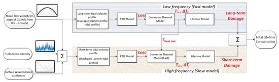
Lifetime analyses for wind energy converters based on active water cooling systems has been widely studied [6,18,19]. Because the passive cooling system is considered here, this means that the lifetime calculation has to be done in a slightly modified manner. This is due to the longer time constant of the passive cooling system. The main methodology is shown in Figure 11. The calculations are performed in time domain. The temperature cycles are then calculated using the rainflow counting algorithm [18,45].

The high thermal capacitance of the enclosure wall makes the thermal models relatively slow in terms of computation time. For the short-term cycling, these computations are accelerated in this paper by assuming that the enclosure wall is at a constant temperature as long as the mean tidal velocity remains constant. The idea is to obtain the wall temperature from the model taking only mean tidal velocity variation into account. This wall temperature information is then used as a boundary condition in the fast converter thermal model to estimate the junction temperature cycling near the power frequency. This is illustrated in Figure 11.

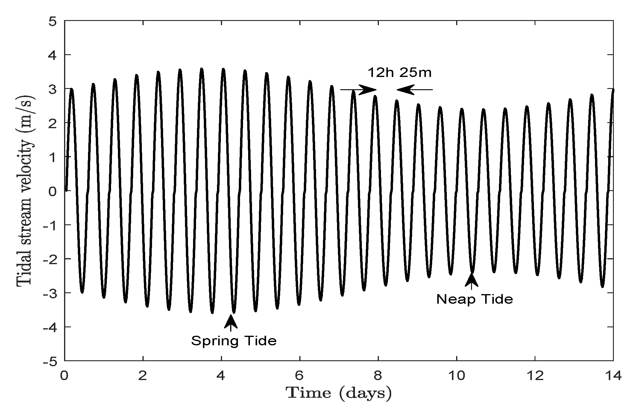
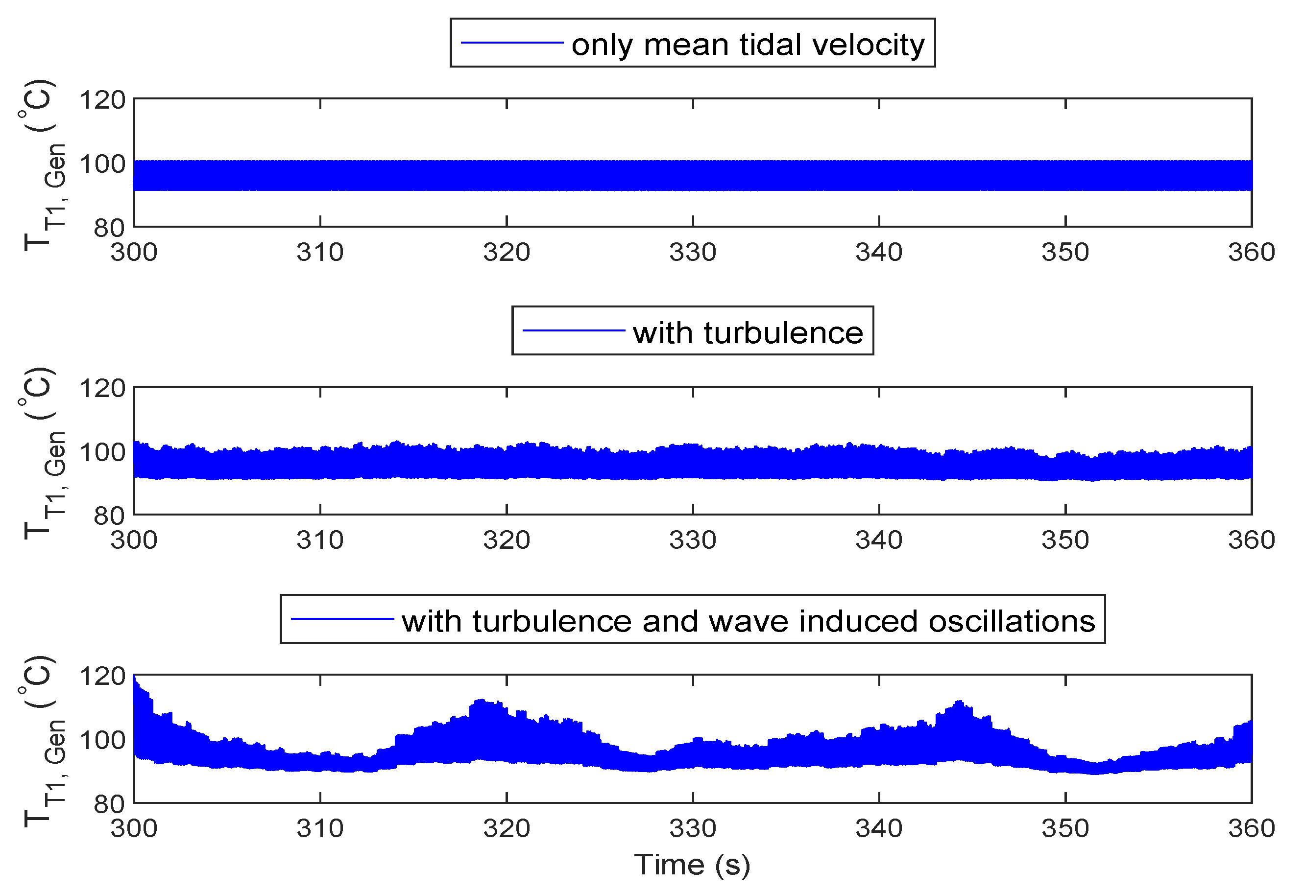
Thermal cycling can be divided into two main categories: long-term and short-term. By long term cycling we mean cycles due to variation in tidal current speeds over 12-hourly cycles, and variations due to the spring and neap tide cycles, as shown in Figure 4. Although monthly and/or yearly variations in the tides can also be included, these have been neglected in this analysis, as their impact is expected to be negligible. Short-term cycling mainly refers to power-frequency thermal cycling and other oscillations due to turbulence and surface waves in the mean tidal stream velocity.

The lifetime estimation in this work has been based on the models presented in References [6,15]. These models give the number of thermal cycles to failure as a function of various parameters, with emphasis on junction temperature cycling and its mean value as per the following equation:

$$\begin{array}{c}\hfill N_f=A·\Delta T_j^{{\beta }_1}·e^{\frac{{\beta }_2}{T_{j,m}+273}}·t_{on}^{{\beta }_3}·I^{{\beta }_4}·V^{{\beta }_5}·D^{{\beta }_6}.\end{array}$$

(6)

$N_f$ is the number of cycles to failure, $T_{j,m}$ is the mean junction temperature, and $t_{on}$ is the on-pulse duration, I current per wire, V is the chip blocking voltage and D is the bonding wire diameter. The constants, A, ${\beta }_1$ to ${\beta }_6$ are obtained from Reference [30], and take the following values: A = 9.34 × 10${}^{14}$ for IGBT4 modules, [${\beta }_1,\cdots ,{\beta }_6$] = [−4.416, 1.285 × 10${}^3$, −0.463, −0.716, −0.761, −0.5].

The lifetime calculation is based on junction temperature of the IGBT and the diode. These values are calculated from the thermal model of the converter explained in the next section. After the calculation of thermal cycles, the number of cycles to failure are calculated based on the Miner’s rule [19]. That is,

$$\begin{array}{c}\hfill \sum _i\frac{n_i}{N_i}=1\end{array},$$

(7)

where, $n_i$ is the number of cycles to failure at the temperature cycle $\Delta T_i$, and $N_i$ is the number of cycles to failures for the same amplitude and same stress type. The number of cycles for each thermal cycling amplitude are obtained from Equation (6). Figure 13 shows how $N_f$ typically varies with $\Delta T_j$ for constant $T_{j,m}$.

Following assumptions have been made in this analysis to reduce the calculation time:

• A constant seawater temperature of 15 ${}^{°}$C was assumed, neglecting variation in annual temperature.
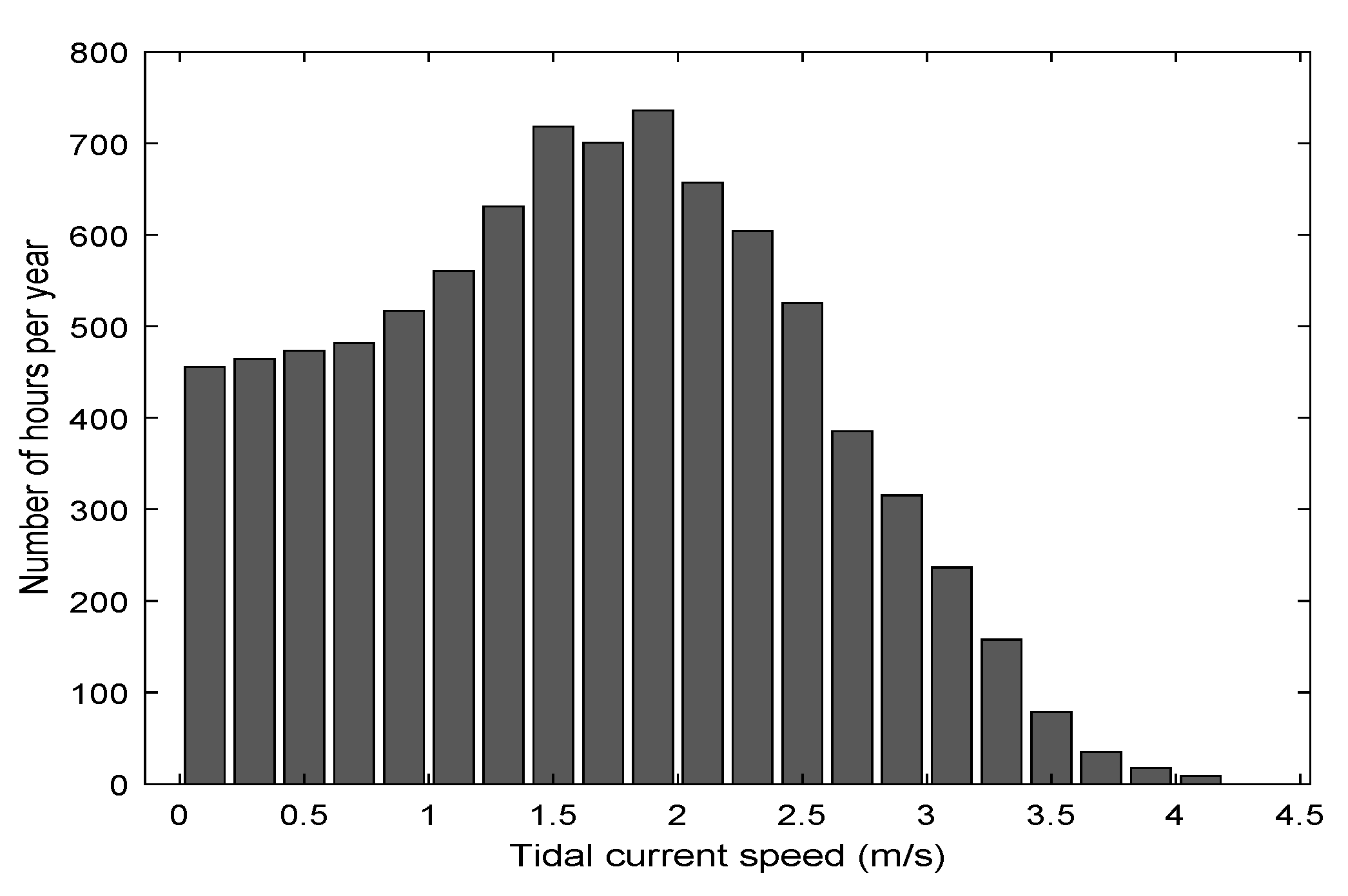
• A constant turbulence value has been used for each mean tidal velocity, as already mentioned in Section 2.
• The turbine under consideration is an active speed stall controlled one, with no yawing capabilities. It is assumed that the performance of the turbine drops negligibly between the flood and ebb tides. Hence, as far as turbine characteristics are concerned, no distinction is made between the flood and ebb tides.
• At the beginning of each flood and ebb tide cycle, the junction temperature of the IGBT module is same as the ambient temperature.
• A constant power factor of operation (0.9) is assumed on the grid-side converter. In other words, effects of varying reactive power on thermal cycling have been neglected [27].

5. Estimation of Junction Temperatures

The mean junction temperature and its amplitude about the mean value are obtained from the thermal models of the passively cooled converter [11]. The losses inside the IGBT and diode comprise of the conduction and the switching losses given by the following equations [27]:

$$\begin{array}{c}\hfill P_{cond,IGBT}=u_{CE}\left(i\right)·i·d_{IGBT},\\ \hfill P_{cond,Diode}=u_F\left(i\right)·i·d_{Diode},\\ \hfill P_{sw,IGBT}=(E_{on,IGBT}+E_{off,IGBT})·f_s,\mathrm{and}\\ \hfill P_{sw,Diode}=(E_{on,Diode}+E_{off,Diode})·f_s\end{array}$$

(8)

where, $P_{cond,k}$ and $P_{sw,k}$ denote the conduction and switching losses respectively in the device ’k’. $u_{CE}$ and $u_F$ represent the forward voltage drops in the IGBT and diode respectively, whereas i is the component current. $d_k$ is the duty ratio of the switch ’k’. And, $E_{on,k}$ and $E_{off,k}$ is the on and off switching energy of the device ’k’; and $f_s$ is the switching frequency. Parameters for the loss calculations can be found in datasheets for IGBT modules in Reference [46]. Details on loss calculation in the IGBT and diodes can be found in multiple references, such as References [6,19,27].

The RC-thermal network of the submerged power converter with IGBT mounted on a Cu mounting plate (see Figure 2) inside the sealed enclosure is shown in Figure 14 [11]. Calculation of the thermal resistances shown in Figure 14 have been explained in Reference [11]. For the sake of brevity, the mathematical details of the thermal model are omitted from this paper. However, a qualitative description is given below.

Heat transfer from the IGBT junction to the ambient seawater encounters three main thermal resistances (networks): IGBT junction-to-case, case-to-external wall, external wall-to-ambient water. The junction-to-case thermal network is represented typically by a 4-layer Foster network given in the datasheet of the IGBT module [46]. However, Foster models cannot be directly connected to the RC-ladder network of the rest of the thermal network. Therefore, a slightly modified approach using a 1-layer equivalent network, as explained in References [11,47] is adopted as shown in Figure 14.

The mounting plate and the enclosure wall thermal impedances include the case-to-external wall impedances. These can be represented by one-dimensional thermal resistance together with the spreading resistances in the mounting plate and the enclosure wall [11,48]. These spreading resistances form the bulk of the thermal resistance in case of the passively cooled submerged power converters. Proper selection of the mounting plate material and dimensions can significantly reduce the spreading resistance, as discussed in Reference [11]. The thermal capacitance calculations of the mounting plate and the wall are simply calculated using the heat capacity of these blocks.

And finally, the wall-to-ambient seawater thermal resistance is calculated using empirical relations [49], and a few steady state computational fluid dynamics (CFD) simulations, as explained in Reference [11]. The convective heat transfer coefficient is a function of the mean power loss and/or wall temperature. The enclosure wall resistance is thus a dynamic variable, and needs to be recalculated continuously.

Whereas for the forced water cooling methods the case to ambient thermal resistance is almost independent of the heat loss in the power module, same cannot be said for the passively cooled converter. For the latter, heat transfer coefficient at the external wall of enclosure is a function of the heat flux from the power module [11]. Commonly encountered values of case to ambient thermal resistance for forced water cooled systems falls in the range of 0.005–0.020 K/W. In this study, depending on the heat loss this thermal resistance falls in the range of 0.02–0.1 K/W. The case to seawater thermal resistance decreases with increase in loss in the power module. Please note that increased thermal resistance in passive cooling is accompanied by improved reliability due to no moving parts.

6. Case Study: Lifetime Analysis of a Tidal Turbine Converter

In this section we apply the lifetime model presented earlier to a 110 kW tidal turbine PTO system, for which the specifications were mentioned in Section 3. The idea is to first demonstrate the speed control algorithm works as expected, and then assess the impact of loading on the lifetime due to various operating conditions the PTO is subjected to.

6.1. Speed Control

Figure 15 shows the corresponding variation in the generator speed against the tidal stream velocity. In Figure 15 the generator is operating at the rated power near cut-off speed of 3.3 m/s. This means that for any increase in the velocity of tidal stream, the generator rpm must drop as a consequence of the active speed stall control to maintain constant power. As expected, for higher fluctuation in tidal stream velocity, the generator speed also varies with higher magnitude.

6.2. Converter Loading

The change in the tidal stream velocity is also reflected as the change in the phase current of the generator. This can be seen in Figure 16. A comparison between Figure 15 and Figure 16 shows that the drop in generator speed is accompanied by the increase in current. In the constant power region, drop in phase emf due to reduced speed is compensated by the increase in current, and vice-versa.

Another observation from Figure 15 is that there is a substantial change in the generator speed as a result of change in tidal stream velocity. This characteristic is particular to tidal turbines controlled by active speed stall. Compare this with the data obtained from a case study of a 10 MW wind turbine, as shown in Figure 17 [6]. Both the 10 MW wind turbine and 110 kW tidal turbine are operating in the region of constant power above the rated wind/tidal speed; whereas wind turbine is pitch-controlled, the tidal turbine is active speed stall controlled. The point to note here is that the fluctuations in wind speed will not be reflected so much in the generator currents as much as the fluctuations in tidal speed would be. This is both a consequence of pitch control as well as the large inertia of the wind turbine rotor over the tidal turbine.

As a result when a pitch controlled wind turbine operates in the region of constant power, its speed is nearly constant and so is the magnitude of the phase currents. However, same cannot be said of an active speed stall controlled tidal turbine, as illustrated in Figure 17. Therefore, significant differences in the lifetime consumption of the power semiconductor devices can be expected in wind and tidal turbines, as a result of change in the incoming wind/tidal current velocity.

6.3. Junction Temperatures

For the corresponding currents shown in Figure 16, the Generator side converter Diode (D1) and IGBT (T1) junction temperatures are shown in Figure 18 and Figure 19 respectively. Figure 18 also shows the zoomed-in version, where power cycling (high frequency) can be seen alongside the low frequency cycling caused by turbulence and surface waves. Similar high frequency cycling will also be observed in Figure 19, however, we omit showing that here for sake of brevity. As expected, the junction temperatures follow a similar trend to the phase currents because the losses increase with increase in current.

The mean junction temperature of the diode increases with the increase in the tidal stream velocity, as shown in Figure 20. At lower tidal velocities, this is because of increase in output power. In the constant power range, the increase in mean junction temperature is inversely related to the generator speed as explained above. Because of this a large portion of lifetime consumption of the power semiconductor devices is expected in the constant power range. In this region high power is accompanied by low generator speed.

The results here are shown only for a 60 s interval for a specific value of mean tidal velocity, turbulence and wave condition. However, the total lifetime analysis is performed over the entire range of the tidal velocity and the wave spectrum (see Table 3 and Table 4), in accordance with Figure 11.

6.4. Lifetime Consumption

Based on the lifetime model presented earlier in Section 4, expected lifetime of the converter is presented in

Table 7. Lifetime Values.

Velocity Type	Lifetime (in Years)
Considering only mean tidal velocity	151.5
With turbulence	67.0
With turbulence and waves	38.2

. The critical component in terms of lifetime was found to be the diode of the generator side converter, which is taken as the lifetime of the converter. For the sake of brevity, results from the grid side converter are not presented in this paper.

Because of the higher fluctuations in the junction temperature due to turbulence and the wave induced oscillations in the tidal stream velocity, the lifetime decreases accordingly. Such significant drop in the lifetime is probably because of the higher speed oscillations of the tidal turbine generator.

Another interesting thing to note here is that even though the lifetime drops significantly because of turbulence in the tidal stream velocity, the difference in annual loss of the converter semiconductor switches with and without turbulence is negligible, as shown in

Table 8. Annual Generator Side Converter Loss (includes losses for all phases).

Velocity Type	Generator IGBTs (in MWh)	Generator Diodes (in MWh)
Considering only mean tidal velocity	2.11	2.53
With turbulence	2.07	2.44

. This also implies that in this case is the magnitude of temperature swing is more responsible for component degradation than the mean value of temperature. The mean junction temperature is a function of the mean power loss. For the waveforms shown in Figure 18, the temperature swings are listed in

Table 9. Diode Temperatures corresponding to Figure 18.

Velocity Type	${\mathit{T}}_{\mathit{j},\mathit{D}1,\mathit{max}}$ (${}^{°}$C)	${\mathit{T}}_{\mathit{j},\mathit{D}1,\mathit{min}}$ (${}^{°}$C)	$\mathbf{\Delta }{\mathit{T}}_{\mathit{j},\mathit{D}1}$ (${}^{°}$C)
Mean tidal velocity	112.4	93.3	18.4
With turbulence	115.5	93.4	21.1
With turbulence and waves	129.6	91.5	38.1

.

Normally the tidal turbines are designed to have a lifetime of 20 years. Therefore, from above results it can be said that passive cooling can provide adequate lifetime as long as the system is properly designed, and devices are properly rated. Moreover, improvements in lifetime can be gained by overrating the devices further, as demonstrated in other studies [6].

6.5. Damage Distribution

To understand the damage distribution better due to turbulence and wave induced speed oscillations, we consider the operation of the tidal turbine near rated speed (2.5 m/s). Assuming no fluctuations in the tidal stream velocity, almost all of the damage is done by the power cycling frequency—that is, frequency of the generator phase currents which is about 20 Hz—as shown in Figure 21.

When turbulence is included in the tidal stream velocity, the damage distribution histogram shows a lot of frequency components in the lower frequency range as seen in Figure 21. This arises because of the lower frequency components in the junction temperatures of the diode when turbulence is included. Furthermore, if a wave induced oscillation from a wave of time period of 11 s is superimposed on the tidal stream velocity with turbulence, the damage distribution is reflected in this frequency range (<0.10 Hz) as well. Therefore, turbulence and wave induced oscillations not only cause more damage but also shift the damage distribution to lower frequency components.

There is another component of thermal cycling or damage not seen in Figure 21. This thermal cycling component arises because of the daily variation of mean tidal velocity as explained in Section 4. The mean junction temperature of the Generator Diode D1 varies with the tidal stream velocity as shown in Figure 20. This low frequency cycling in the mean junction temperature is what we refer to as long term damage. The frequency and magnitude of long term cycling depends on the history of the mean tidal velocity. In other words, the amplitude and period of each long term cycle depends on whether it was a spring or a neap tide cycle; this was highlighted in Section 2.

The net lifetime damage due to long term cycling is constant irrespective of whether turbulence and waves are included or not. Therefore, the damage contribution in percentage from long term cycling is less when other effects such as turbulence or waves are not accounted for, as seen in

Table 10. Lifetime Values.

Velocity Type	Damage from Daily Cycling (%)
Considering only mean tidal velocity	27
With turbulence	12
With turbulence and waves	6.9

.

7. Conclusions

The purpose of this paper was to investigate the thermal cycling failures in IGBT modules for tidal turbine power converters. The converter is submerged and passively cooled by seawater. Results indicate that in such a converter significant reduction in lifetime of the IGBT modules can occur because of the turbulence and surface waves. Daily variations in the mean tidal velocity also contribute, albeit little, to the reduction in lifetime. It was observed that passive cooling can yield adequate lifetime for the IGBT modules in tidal turbine converters. Whereas passive cooling is less prone to failure than forced water cooling methods, the latter can provide better cooling. On the other hand, passive cooling on account of its reliability can minimize maintenance expenses, and reduce cost of energy in the long term. Unless even the most optimally designed passive cooling system proves inadequate, forced cooling methods should not necessarily be the first choice. Furthermore, passive cooling systems have longer thermal time constants than forced cooling systems, which would mean longer computation time for the thermal models. Therefore, this paper used a modified approach to reduce the computation time by dividing the thermal model into low and high frequency models.

References

1. Vedachalam, N.; Babu, S.; Ramadass, G.; Atmanand, M. Review of maturing multi-megawatt power electronic converter technologies and reliability modeling in the light of subsea applications. Appl. Ocean Res. 2014, 46, 28–39. [Google Scholar] [CrossRef]
2. Magagna, D.; Monfardini, R.; Uihlein, A. JRC Ocean Energy Status Report; European Commission: Luxembourg, 2016. Available online: https://setis.ec.europa.eu/sites/default/files/reports/ocean_energy_report_2016.pdf (accessed on 20 December 2019).
3. Carroll, J.; McDonald, A.; McMillan, D. Reliability comparison of wind turbines with DFIG and PMG drive trains. IEEE Trans. Energy Convers. 2014, 30, 663–670. [Google Scholar] [CrossRef] [Green Version]
4. CATAPULT. Portfolio Review 2016: System Performance, Availability and Reliability Trends Analysis (SPARTA). 2017. Available online: https://s3-eu-west-1.amazonaws.com/media.ore.catapult/wp-content/uploads/2017/03/28102600/SPARTAbrochure_20March-1.pdf (accessed on 1 January 2020).
5. Fischer, K.; Pelka, K.; Puls, S.; Poech, M.; Mertens, A.; Bartschat, A.; Tegtmeier, B.; Broer, C.; Wenske, J. Exploring the causes of power-converter failure in wind turbines based on comprehensive field-data and damage analysis. Energies 2019, 12, 593. [Google Scholar] [CrossRef] [Green Version]
6. Shipurkar, U.; Lyrakis, E.; Ma, K.; Polinder, H.; Ferreira, J. Lifetime comparison of power semiconductors in three-level converters for 10 MW wind turbine systems. IEEE J. Emerg. Sel. Top. Power Electron. 2018, 6, 1366–1377. [Google Scholar] [CrossRef]
7. Hu, Y.; Shi, P.; Li, H.; Yang, C. Health condition assessment of base-plate solder for multi-chip IGBT module in wind power converter. IEEE Access 2019, 7, 72134–72142. [Google Scholar] [CrossRef]
8. Qian, C.; Gheitaghy, A.; Fan, J.; Tang, H.; Sun, B.; Ye, H.; Zhang, G. Thermal management on IGBT power electronic devices and modules. IEEE Access 2018, 6, 12868–12884. [Google Scholar] [CrossRef]
9. Yang, Y.; Wang, H.; Sangwongwanich, A.; Blaabjerg, F. Design for reliability of power electronic systems. In Power Electronics Handbook, 4th ed.; Elsevier: Oxford, UK, 2018; pp. 1423–1440. [Google Scholar]
10. Tavner, P.; Xiang, J.; Spinato, F. Reliability analysis for wind turbines. Wind Energy 2007, 10, 1–18. [Google Scholar] [CrossRef]
11. Wani, F.; Shipurkar, U.; Dong, J.; Polinder, H. A study on passive cooling in subsea power electronics. IEEE Access 2018, 6, 67543–67554. [Google Scholar] [CrossRef]
12. Toma, D.; Mànuel-Làzaro, A.; Nagueras, M.; Del Rio, J. Study on heat dissipation and cooling optimization of the junction box of OBSEA seafloor observatory. IEEE/ASME Trans. Mechatron. 2014, 20, 1301–1309. [Google Scholar] [CrossRef] [Green Version]
13. Liu, M.; Li, W.; Wang, C.; Billinton, R.; Yu, J. Reliability evaluation of a tidal power generation system considering tidal current speeds. IEEE Trans. Power Syst. 2016, 31, 3179–3188. [Google Scholar] [CrossRef]
14. Ren, Z.; Li, H.; Li, W.; Zhao, X.; Sun, Y.; Li, T.; Jiang, F. Reliability evaluation of tidal current farm integrated generation systems considering wake effects. IEEE Access 2018, 6, 52616–52624. [Google Scholar] [CrossRef]
15. Bayerer, R.; Herrmann, T.; Licht, T.; Lutz, J.; Feller, M. Model for power cycling lifetime of IGBT modules—Various factors influencing lifetime. In Proceedings of the 5th International Conference on Integrated Power Systems (CIPS), Nuremberg, Germany, 11–13 March 2008; pp. 1–6. [Google Scholar]
16. Musallam, M.; Johnson, C.M.; Yin, C.; Lu, H.; Bailey, C. Real-time life expectancy estimation in power modules. In Proceedings of the 2nd Electronics System-Integration Technology Conference, Greenwich, UK, 1–4 September 2008; pp. 231–236. [Google Scholar]
17. Kovacevic-Badstuebner, I.F.; Kolar, J.W.; Schilling, U.; Chung, H.; Wang, H.; Blaabjerg, F.; Pecht, M. Modelling for the lifetime prediction of power semiconductor modules. In Reliability of Power Electronic Converter Systems; IET: London, UK, 2015; pp. 103–140. [Google Scholar]
18. Ikonen, M. Power Ccling Lifetime Estimation of IGBT Power Modules Based on Chip Temperature Modeling. Ph.D. Thesis, Lappeenranta University of Technology, Lappeenranta, Finland, 2012. [Google Scholar]
19. Ma, K.; Liserre, M.; Blaabjerg, F.; Kerekes, T. Thermal loading and lifetime estimation for power device considering mission profiles in wind power converter. IEEE Trans. Power Electron. 2015, 30, 590–602. [Google Scholar] [CrossRef]
20. Givaki, K.; Parker, M.; Jamieson, P. Estimation of the power electronic converter lifetime in fully rated converter wind turbine for onshore and offshore wind farms. In Proceedings of the 7th IET International Conference on Power Electronics, Machines and Drives (PEMD), Manchester, UK, 8–10 April 2014. [Google Scholar]
21. Ma, K.; Liserre, M.; Blaabjerg, F. Reactive power influence on the thermal cycling of multi-MW wind power inverter. IEEE Trans. Ind. Appl. 2013, 49, 922–930. [Google Scholar] [CrossRef]
22. Zhou, D.; Blaabjerg, F.; Lau, M.; Tønnes, M. Optimized reactive power flow of DFIG power converters for better reliability performance considering grid codes. IEEE Trans. Ind. Electron. 2014, 62, 1552–1562. [Google Scholar] [CrossRef]
23. Ma, K.; Blaabjerg, F. Multilevel converters for 10 MW wind turbines. In Proceedings of the 14th European Conference on Power Electronics and Applications, Birmingham, UK, 30 August–1 September 2011; pp. 1–10. [Google Scholar]
24. Andresen, M.; Ma, K.; Buticchi, G.; Falck, J.; Blaabjerg, F.; Liserre, M. Junction temperature control for more reliable power electronics. IEEE Trans. Power Electron. 2017, 33, 765–776. [Google Scholar] [CrossRef] [Green Version]
25. Chen, G.; Cai, X. Adaptive control strategy for improving the efficiency and reliability of parallel wind power converters by optimizing power allocation. IEEE Access 2018, 6, 6138–6148. [Google Scholar] [CrossRef]
26. Andresen, M.; Kurpat, J.; Raveendran, V.; Falck, J.; Liserre, M. Active thermal control for delaying maintenance of power electronics converters. Chin. J. Electr. Eng. 2018, 33, 13–20. [Google Scholar]
27. Shipurkar, U. Improving the Availability of Wind Turbine Generator Systems. Ph.D. Thesis, Delft University of Technology, Delft, The Netherlands, 2019. [Google Scholar]
28. Rajashekara, K.; Krishnamoorthy, H.; Satish, B. Electrification of subsea systems: Requirements and challenges in power distribution and conversion. CPSS Trans. Power Electron. Appl. 2017, 2, 259–266. [Google Scholar] [CrossRef]
29. Hernes, M.; Pittini, R. Enabling pressure tolerant power electronic converters for subsea applications. In Proceedings of the 13th European Conference on Power Electronics and Applications, Barcelona, Spain, 8–10 September 2009; pp. 1–10. [Google Scholar]
30. Wintrich, A.; Nicolai, U.; Tursky, W.; Reimann, T. Application Manual Power Semiconductors. SEMIKRON International GmbH. 2015. Available online: https://www.semikron.com/dl/service-support/downloads/download/semikron-application-manual-power-semiconductors-english-en-2015/ (accessed on 30 October 2019).
31. CATAPULT. ReDAPT—Public Domain Report: Final (MC7.3). Technical Report. 2015. Available online: http://redapt.eng.ed.ac.uk/library/eti/reports/MC7.3%20Operations%20Final%20Report.pdf (accessed on 5 January 2020).
32. Sellar, B.; Wakelam, G.; Sutherland, D.; Ingram, D.; Venugopal, V. Characterisation of tidal flows at the european marine energy centre in the absence of ocean waves. Energies 2018, 11, 176. [Google Scholar] [CrossRef] [Green Version]
33. Jonkman, B.; Kilcher, L. Turbsim User’s Guide: Version 1.06.00. National Renewable Energy Laboratories: Golden, CO, USA. Available online: https://nwtc.nrel.gov/TurbSim (accessed on 25 September 2019).
34. Zhou, Z.; Scuiller, F.; Charpentier, J.F.; Benbouzid, M.; Tang, T. Power smoothing control in a grid-connected marine current turbine system for compensating swell effect. IEEE Trans. Sustain. Energy 2013, 4, 816–826. [Google Scholar] [CrossRef] [Green Version]
35. Zhou, Z.; Benbouzid, M.; Charpentier, J.F.; Scuiller, F.; Tang, T. A review of energy storage technologies for marine current energy systems. Renew. Sustain. Energy Rev. 2013, 18, 390–400. [Google Scholar] [CrossRef] [Green Version]
36. Techet, A. MIT Ocean Engineering: Ocean Waves. Available online: https://ocw.mit.edu/courses/mechanical-engineering/2-22-design-principles-for-ocean-vehicles-13-42-spring-2005/readings/lec6_wavespectra.pdf (accessed on 20 December 2019).
37. BS 6349: Part 1: Maritime Structures—Code of Practice for General Criteria; British Standards Institution: London, UK, 2000.
38. Lavidas, G.; Venkatesan, V. Characterising the wave power potential of the scottish coastal environment. Int. J. Sustain. Energy 2017, 37, 684–703. [Google Scholar] [CrossRef]
39. Climate-data.org. Climate: Kirkwall. Available online: https://en.climate-data.org/location/56552/ (accessed on 5 March 2018).
40. Whitby, B.; Ugalde-Loo, C.E. Performance of pitch and stall regulated tidal stream turbines. IEEE Trans. Sustain. Energy 2014, 5, 64–72. [Google Scholar] [CrossRef]
41. Polinder, H.; Bang, D.; Van Rooij, R.; McDonald, A.; Mueller, M. 10 MW wind turbine direct-drive generator design with pitch or active speed stall control. In Proceedings of the IEEE International Electric Machines and Drives Conference, Antalya, Turkey, 3–5 May 2007; pp. 1390–1395. [Google Scholar]
42. Djebarri, S.; Charpentier, J.F.; Scuiller, F.; Benbouzid, M. A systemic design methodology of PM generators for fixed-pitch marine current turbine. In Proceedings of the 1st International Conference on Green Energy, Sfax, Tunisia, 25–27 March 2014; pp. 32–37. [Google Scholar]
43. Zhou, Z.; Scuiller, F.; Charpentier, J.F.; El, M.; Benbouzid, H.; Tang, T. Power control of a non-pitchable PMSG-based marine current turbine at overrated current speed with flux-weakening strategy. IEEE J. Ocean. Eng. 2015, 40, 536–545. [Google Scholar] [CrossRef] [Green Version]
44. Ma, K. Electro-thermal model of power semiconductors dedicated for both case and junction temperature estimation. In Power Electronics for the Next Generation Wind Turbine System; Springer: Cham, Switzerland; London, UK, 2015; pp. 139–143. [Google Scholar]
45. Denk, M.; Bakran, M.M. Comparison of counting algorithms and empiric lifetime models to analyze the load-profile of an IGBT power module in a hybrid car. In Proceedings of the IEEE 2013 3rd International Electric Drives Production Conference (EDPC), Nuremberg, Germany, 29–30 October 2013; pp. 1–6. [Google Scholar]
46. Infineon Technologies. IGBT Modules. Available online: https://www.infineon.com/cms/en/product/power/igbt/igbt-modules/ (accessed on 15 September 2019).
47. Ma, K.; Yang, Y.; Blaabjerg, F. Transient modelling of loss and thermal dynamics in power semiconductor devices. In Proceedings of the Energy Conversion Congress and Exposition (ECCE), Pittsburg, PA, USA, 14–18 September 2014; pp. 5495–5501. [Google Scholar]
48. Muzychka, Y.; Culham, J.; Yovanovich, M. Thermal spreading resistance of eccentric heat sources on rectangular flux channels. J. Electron. Packag. 2003, 125, 178–185. [Google Scholar] [CrossRef]
49. Cengel, Y.; Ghajar, A.J. Heat and Mass Transfer, Fundamentals & Application; McGraw-Hill: New York, NY, USA, 2014. [Google Scholar]
Figure 1. Tidal turbine drive train with a direct-drive permanent magnet synchronous generator (PMSG) and a power electronic (PE) converter.
Energies 13 01875 g001
Figure 2. Power electronic module in a submerged and hermetically-sealed power converter [11].
Energies 13 01875 g002
Figure 3. Tidal velocity distribution at EMEC site, Orkney [31].
Energies 13 01875 g003
Figure 4. Tidal stream velocity profile at a typical tidal site experiencing semi-diurnal tides.
Energies 13 01875 g004
Figure 5. Fluctuations in tidal stream velocity about its mean value (here taken as 3.3 m/s) as a consequence of turbulence and wave induced oscillations.
Energies 13 01875 g005
Figure 6. Annual sea temperature ranges at Kirkwall near Orkney, UK. The black curve in the middle of the shaded area represents the average temperature. Data source: Reference [39].
Energies 13 01875 g006
Figure 7. C p λ curve for the tidal turbine; adapted from Reference [43].
Energies 13 01875 g007
Figure 8. Power curve of the fixed pitch tidal turbine as a function of the tidal stream velocity.
Energies 13 01875 g008
Figure 9. Speed curve of the fixed pitch tidal turbine as a function of the tidal stream velocity.
Energies 13 01875 g009
Figure 10. Representative diagram of a 2-level back-to-back voltage source converter (2L-VSC).
Energies 13 01875 g010
Figure 11. Methodology for lifetime calculations. Finer details of the power take-off (PTO) model are shown in Figure 12.
Energies 13 01875 g011
Figure 12. Internal structure of the PTO model.
Energies 13 01875 g012
Figure 13. Number of cycles to failure are presented as a function of temperature cycling for a constant mean junction temperature.
Energies 13 01875 g013
Figure 14. Lumped element thermal network model for the system shown in Figure 2 [11].
Energies 13 01875 g014
Figure 15. Active speed stall control of Generator speed as a function of change in tidal stream velocity. Mean tidal velocity in this image is set at 3.3 m/s.
Energies 13 01875 g015
Figure 16. Generator phase currents (RMS values).
Energies 13 01875 g016
Figure 17. Comparison of generator speed fluctuations in a 10 MW wind turbine and a 110 kW tidal turbine.
Energies 13 01875 g017
Figure 18. Temperature of the Generator Side Converter Diode (D1) as a function of the fluctuations in the tidal stream velocity.
Energies 13 01875 g018
Figure 19. Temperature of the Generator Side Converter insulated gate bipolar transistor (IGBT) (T1) as a function of the fluctuations in the tidal stream velocity.
Energies 13 01875 g019
Figure 20. Mean junction temperature of Generator Side Converter Diode.
Energies 13 01875 g020
Figure 21. Percentage of total damage vs. frequency of thermal cycling, when turbulence and surface wave (Hs = 5.75 m, Tp = 11 s) is superimposed to the mean tidal velocity of 2.5 m/s.
Energies 13 01875 g021