Abstract
In this paper, a multi-phase multi-time-scale real-time dynamic active-reactive optimal power flow (RT-DAR-OPF) framework is developed to optimally deal with spontaneous changes in wind power in distribution networks (DNs) with battery storage systems (BSSs). The most challenging issue hereby is that a large-scale ‘dynamic’ (i.e., with differential/difference equations rather than only algebraic equations) mixed-integer nonlinear programming (MINLP) problem has to be solved in real time. Moreover, considering the active-reactive power capabilities of BSSs with flexible operation strategies, as well as minimizing the expended life costs of BSSs further increases the complexity of the problem. To solve this problem, in the first phase, we implement simultaneous optimization of a huge number of mixed-integer decision variables to compute optimal operations of BSSs on a day-to-day basis. In the second phase, based on the forecasted wind power values for short prediction horizons, wind power scenarios are generated to describe uncertain wind power with non-Gaussian distribution. Then, MINLP AR-OPF problems corresponding to the scenarios are solved and reconciled in advance of each prediction horizon. In the third phase, based on the measured actual values of wind power, one of the solutions is selected, modified, and realized to the network for very short intervals. The applicability of the proposed RT-DAR-OPF is demonstrated using a medium-voltage DN.
1. Introduction
There is a strong demand for increasing the penetration level of wind energy into distribution networks (DNs). However, a considerable amount of this generation may need to be curtailed due to technical constraints in the network. Battery storage systems (BSSs) can be optimally used to store the energy, decrease the curtailment, and consequently increase economic benefits. However, BSSs introduce dynamic terms to the problem of optimal power flow (OPF). In addition, considering both the active and reactive power capability of the BSSs with flexible operation strategies, as well as maximizing the lifetime of the batteries further increases the complexity of the problem. Furthermore, wind power is intermittent, and therefore the network operator has to quickly update the operation strategies correspondingly. This task should be carried out by a ‘real-time’ optimization aiming at determining a huge number of mixed-integer decision variables. Therefore, a real-time dynamic active-reactive OPF (RT-DAR-OPF) problem should be solved to ensure not only optimality but also the feasibility of the system operation.
RT-OPF was first introduced in [1] and then attracted the interest of many studies: [2] introduced a real-time strategy based on a linear model predictive control (MPC) for OPF in the presence of BSSs and wind turbines; [3] utilized neural networks for RT-OPF in radial DNs considering uncertain demand and renewable energy generation (REGs); [4] developed two real-time algorithms for constraint satisfaction for OPF; [5] proposed an RT-OPF control approach based on a feedback mechanism; [6] proposed a risk-based RT-OPF considering uncertain REGs; [7] developed a data-driven hourly real-time power dispatch framework; [8] proposed an online gradient algorithm for OPF on radial networks ensuring low computation time; [9] proposed an RT-OPF algorithm based on quasi-Newton methods; [10] proposed an RT-OPF approach considering the minute-to-minute variability of REGs and demand; [11] developed a feedback controller for photovoltaic inverters seeking OPF solutions; [12] extended the research in [11] by improving the convergence properties of the feedback controllers for the case of time-varying ambient and network conditions; [13] developed a prediction-realization RT-OPF framework to deal with intermittent wind power in DNs; [14] extended the framework in [13] by incorporating the reactive power dispatch of wind farms (WFs) as well as overcoming convergence issues [15] by introducing a reconciliation algorithm; [16] utilized graphical processing units to accelerate the OPF computation; [17] presented a real-time optimization method for alleviating contingencies (e.g., line overloads and voltage limit violations) in transmission networks; [18] proposed a multi-stage stochastic optimization for real-time economic dispatch of storage (specifically pumped hydro) resources; [19] proposed a feedback-based RT-OPF algorithm to satisfy technical constraints in real time; and [20] proposed an MPC-based distributed RT-OPF method for interconnected microgrids. For a detailed survey of RT-OPF methods, we refer to [21]. It is noted that all the above studies on ‘real-time’ OPF [1,2,3,4,5,6,7,8,9,10,11,12,13,14,15,16,17,18,19,20] did not consider the optimal operations of BSSs when optimizing mixed-integer decision variables of the network.
BSSs could play a significant role in the efficient operation of energy networks. They can lead to a decrease in power losses and voltage deviations [22], supplying peak demand [23,24] by storing the energy instead of energy curtailment [25]. However, the optimal integration of the BSSs into energy networks still needs further investigations. From an operation point of view, the BSSs can be scheduled in a fixed or flexible manner. For instance, [26] utilized both the active and reactive power capability of BSSs [27,28] in the OPF problem based on a fixed length of charge and discharge periods in a prediction horizon. The reactive power provision of distributed energy resources leads to significant economic (e.g., exporting reactive power to an upstream network [14]) and technical benefits (e.g., management of line losses and voltage regulation [29,30]). In [31], it was proposed that BSSs are operated with a flexible length of charge and discharge periods, but identical operation strategies were obtained for different BSSs so as to reduce the number of mixed-integer decision variables. However, realizing the identical solutions for all BSSs (at different locations) cannot be efficient. Therefore, the work in [31] was extended in [32,33] to find optimal operation strategies for each individual BSS. Recently, [34] proposed a multi-period [35,36,37,38] framework to solve the dynamic OPF problem for distribution networks with BSSs under uncertain renewable energy generation. It is noted that the OPF problems in [26,31,32,33,35,36,37,38] were not solved in real time and they did not optimize the depth of discharge (DoD) of BSSs while determining flexible operation strategies. Evaluating expended life costs of batteries based on cycle counting only is not conclusive, and therefore, the DoD of BSSs should also be taken into account [39]. Flexible operation of BSSs and considering both DoD and the number of charge-discharge cycles in the calculation of expended life costs of batteries lead to more efficient operation of BSSs but highly complex dynamic MINLP AR-OPF, in particular when all mixed-integer decision variables are simultaneously optimized. The incorporation of expended life costs of batteries (in terms of both DoD and number of cycles) into ‘real-time’ OPF has not been considered yet. Therefore, this study aimed to develop a new approach with the following contributions over the above literature:
- (1)
- A multi-time-scale dynamic (i.e., with difference equations rather than only algebraic equations) AR-OPF framework is developed to optimally react to the spontaneous changes in wind power and ensure the feasibility of operations in real time when BSSs exist in DNs.
- (2)
- The framework offers the possibility of simultaneous optimization of all of the following mixed-integer variables in a prediction horizon:
- Wind power curtailment of each WF (continuous);
- Active power charge/discharge of each BSS (continuous);
- Reactive power dispatch of each WF and BSS (continuous);
- Length of charge and discharge periods of each BSS (discrete);
- Length of charge-discharge cycles of each BSS (discrete);
- Number of charge-discharge cycles of each BSS in the prediction horizon (discrete);
- Status of charge/discharge of each BSS (binary);
- Slack bus voltage (discrete); and
- Active-reactive reverse power flow to an upstream network (continuous).
- (3)
- Fully flexible optimal operation strategies for BSSs are determined for the dynamic AR-OPF while minimizing the expended life costs of the BSSs as a function of DoD and the number of charge-discharge cycles.
The remainder of the paper is organized as follows. The formulation of a general stochastic dynamic MINLP optimization problem is provided in Section 2. Section 3 describes the proposed RT-DAR-OPF problem. In Section 4, different modes of operations for BSSs are defined and the dynamic MINLP AR-OPF problem is formulated in detail. The results of a case study and conclusions are provided in Section 5 and Section 6, respectively.
2. Problem Formulation
The aim of the RT-DAR-OPF is to compute optimal operation strategies to be realized to DNs with BSSs under uncertain penetration of wind power. A general formulation of the optimization problem can be expressed as:
where is the objective function to be minimized, is the vector of state variables, is the vector of continuous decision variables, is the vector of discrete decision variables, is the vector of binary decision variables, is the vector of random variables, and is time. The objective function is subject to equality and inequality constraints. Here, denotes dynamic nonlinear model equations, denotes the initial states at , are the lower/upper limits on state variables, are the lower/upper limits on continuous decision variables, and is the final time. Equation (1) is a large-scale complex stochastic dynamic MINLP optimization problem, which is difficult to solve.
3. Real-Time Dynamic AR-OPF Framework
To solve the optimization problem Equation (1), we propose a multi-phase multi-time-scale RT-DAR-OPF framework as illustrated in Figure 1. The framework consists of three phases (phases 2 and 3 are adapted from [13,14]) with three different time scales (e.g., , , and ) and 15 steps as follows:
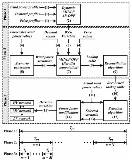
Figure 1.
The proposed framework for RT-DAR-OPF.
- (1)
- Provide hourly forecasted wind power, demand, and price profiles in advance of each prediction horizon .
- (2)
- Solve the corresponding dynamic MINLP AR-OPF problem. In this step, optimal flexible operation strategies for BSSs are computed for the upcoming (e.g., 24 h, with hourly discretization). The detailed problem formulation is described in Section 4.
- (3)
- The variables of BSSs computed in phase 1 will be used as fixed input parameters for the second phase. Note that other decision variables will be recomputed in phase 2.
- (4)
- Provide forecasted values of wind power, demand, and price ahead of each prediction horizon (e.g., 2 min). Note that the length of the prediction horizon should depend on the availability of the forecasted data as well as the computation time in step (7).
- (5)
- To describe uncertain wind power, generate wind power scenarios for each WF using a continuous bounded stochastic distribution with an identical probability between two adjacent scenarios. For this purpose, intervals are defined for the wind power , , such that:where and are the indices for WFs and wind power scenarios, respectively. Pr is the probability operator and the scenarios are margins of the defined intervals. To this end, wind power scenarios are generated for each WF. Then, wind power scenario combinations are formed for each prediction horizon . The total number of scenario combinations will be:where is the total number of WFs.
- (6)
- Send the generated wind power scenario combinations (obtained in step 5) to the MINLP AR-OPF.
- (7)
- Solve the MINLP AR-OPF problems corresponding to each scenario combination for the upcoming . Note that the optimization problems at this step are not dynamic as the optimal operation strategies of BSSs are already given as input parameters. Since reactive power flow has influence on nodal voltages [40,41], the reactive power dispatch of the WFs can lead to voltage violations, in particular when the wind power fluctuates. For this reason, we use a back-off strategy [14] to satisfy voltage constraints in the RT-OPF. Since the optimization problems in this step are independent, they are solved using parallel computation in order to ensure that the solutions for all the scenario combinations are available within the prediction horizon .
- (8)
- Send the solutions of the MINLP AR-OPF problems (obtained in step 7) as a lookup table to a reconciliation algorithm.
- (9)
- Using the reconciliation algorithm, reconcile the lookup table by substituting the un-converged problems with solutions by which the safety of the operations is ensured while minimizing the degree of conservatism.
- (10)
- Send the reconciled lookup table for the to a selection algorithm.
- (11)
- Provide the values of wind power measured at each sampling interval (e.g., 20 s) to the selection and power factor modification algorithms.
- (12)
- The selection algorithm selects a solution strategy based on the measured values of wind power for each sampling interval . The selected scenario ensures the safety of the operation with the minimum of the objective function.
- (13)
- Send the selected scenario to the power factor modification algorithm.
- (14)
- Modify the power factor of WFs before realizing the solution using the power factor modification algorithm. Due to the possible difference between the measured wind power and the selected scenario, realizing the reactive power dispatch can lead to violations of power factor limits. Therefore, the power factor modification algorithm ensures satisfaction of the power factor constraints.
- (15)
- Send the decision variables to the network at each sampling interval .
The above 15 steps are repeated for the next so that the proposed real-time framework aims to autonomously update the operation strategies according to spontaneous changes of the wind power while optimally managing the operation of BSSs.
4. Dynamic MINLP AR-OPF
4.1. Operation Modes of BSSs
It was shown in [39] that the lifetime of a battery is strongly influenced by the DoD and the number of charge-discharge cycles in the prediction horizon. Therefore, in many studies [26,31,32,33], was limited in order to increase the lifetime. Considering this limitation, three types of operation modes can be defined for BSSs in active-reactive OPF as shown in Figure 2.
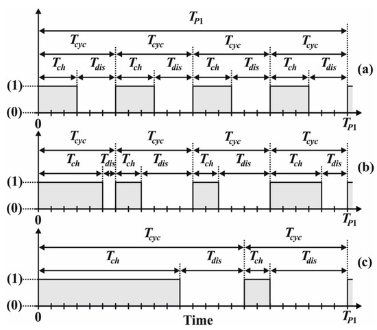
Figure 2.
Different operation modes for BSSs: (a) Mode1, (b) Mode 2, (c) Mode 3.
Mode 1 [26]: Fixed charge and discharge periods, and a fixed number of charge-discharge cycles in the prediction horizon . In this operation mode, the decision variables of the BSSs are , and .
Mode 2 [31,32,33]: Flexible charge and discharge periods, and a fixed number of charge-discharge cycles in the prediction horizon . In this operation mode, the decision variables of the BSSs are , , , , and
.
Mode 3 (proposed): Flexible charge and discharge periods and optimal number of charge-discharge cycles in the prediction horizon . In this operation mode, the decision variables of the BSSs are , , , , , , and .
It can be seen that mode 3 allows higher flexibility compared to the other modes of operation. However, it leads to higher complexity as the number of decision variables in the optimization problem increases. Therefore, in this paper, the dynamic AR-OPF is formulated and a solution approach is presented for BSSs to operate in mode 3. For comparison purposes, we also tested our new framework with the other operation modes in the case study.
4.2. Detailed Problem Formulation
The dynamic optimization problem in phase 1 of the RT-DAR-OPF framework is formulated as follows:
The objective function in Equation (4) minimizes the total costs of active and reactive energy and imported from an upstream network, and meanwhile minimizes the total expended life costs of the BSSs . The significance of our proposed dynamic AR-OPF is that all continuous, discrete, and binary decision variables are simultaneously optimized for the prediction horizon . Here, the vector of continuous decision variables includes curtailment factors of WFs , reactive power dispatch of WFs , active power charge of BSSs , active power discharge of BSSs , and reactive power dispatch of BSSs . The vector of discrete decision variables includes slack bus voltage , charge periods of the BSSs , discharge periods of the BSSs , length of charge-discharge cycles of batteries , and number of charge-discharge cycles of the BSSs in the prediction horizon . The vector of binary decision variables includes , which represents the status of charge/discharge for each BSS.
Equation (4) is subject to the following equality and inequality constraints:
where Equations (5) and (6) are the active and reactive power flow equations at the buses, respectively. Here, and denote the network’s active and reactive power functions [26]. The active-reactive power constraints at the slack bus are:
The nodal voltages are constrained as follows [13,14]:
The feeder limits are:
The constraints of the curtailment factors of WFs are:
and the constraints of the power factors of WFs are:
4.3. Equations of BSSs
In this work, with the aid of power conditioning systems (PCSs), the BSSs can provide and absorb both active and reactive power. The active power charge and discharge are constrained to the capacity of the PCSs:
The reactive power dispatch of the BSSs is constrained to:
The apparent power of the BSSs is constrained to:
Here, we define a binary decision variable to avoid charge and discharge at the same time:
where indicates the charging of the battery while denotes the discharging operation. The energy level of a BSS is calculated as follows:
where Equation (26) shows the dynamic behavior of a battery with initial states in Equation (27).
The ELC of each BSS [39] is a function of the number of cycles in the prediction horizon as well as the average value of the depth of discharge:
where:
In Equations (29) and (33), can be calculated as follows:
where:
.
5. Case Study
In this paper, a 41-bus medium voltage DN [14,26,31,42] is used as a case study to demonstrate the effectiveness of the proposed approach. Two WFs (each with rated power of 10 MW) and two BSSs are located at buses 2 and 16, respectively. The input data for the case study is adapted from [14,39] and given in Table 1 as well as subplots (a)-(c) in Figure 3 and Figure 4. The dynamic MINLP optimization problem in phase 1 is solved using the SBB solver and the optimization problems in phase 2 are solved using the BONMIN solver in GAMS.

Table 1.
Data for the case study taken and adapted from [14,39].
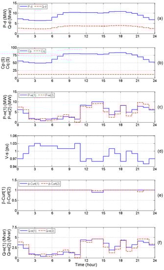
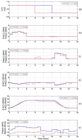
Figure 3.
(a) Total active and reactive power demand; (b) Energy prices; (c) Wind power; (d) Slack bus voltage; (e) Curtailment factors of WFs; (f) Capacitive reactive power of WFs; (g) Binary variables for charge/discharge of BSSs; (h),(i) Active power charge and discharge of BSSs, respectively; (j) Capacitive reactive power of BSSs; (k) Energy levels in BSSs; (l) Active and reactive power at the slack bus.
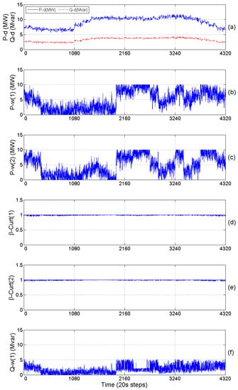
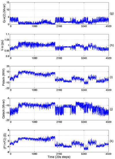
Figure 4.
(a) Total active and reactive power demand; (b),(c) Actual wind power of the first and second WF; (d),(e) Curtailment factors of the first and second WF, respectively; (f) Capacitive reactive power dispatch of the first WF; (g) Capacitive reactive power dispatch of the second WF; (h) Slack bus voltage; (i) Active power at the slack bus; (j) Reactive power at the slack bus; (k) Total costs of active and reactive energy at the slack bus.
Subplots (d)–(l) in Figure 3 show the output of the dynamic MINLP AR-OPF solved in phase 1. The length of the prediction horizon is 24 h with hourly discretization and the maximum number of cycles in the prediction horizon is 4 [39]. Based on the forecasted profiles, all the mixed-integer variables are simultaneously solved for the upcoming day.
In Figure 3, subplot (d) shows the optimal values of the slack bus voltage, taking discrete values with the steps of 0.01 pu. Subplot (e) of Figure 3 confirms that using BSSs in the network can lead to a significant reduction of the wind power curtailment. In the same figure, subplots (g)–(i) shows that using the proposed method, the BSSs could operate with dissimilar strategies in the prediction horizon. Subplots (f) and (j) of Figure 3 show that utilizing the reactive power capability of the WFs and BSSs can lead to a huge amount of reactive power generation in the network. Beside the demand and wind power profiles, energy prices play a significant role in determining the optimal operations of BSSs. It means the batteries tend to be charged when the active energy price is low and discharged when it is high. In addition, the BSSs also dispatch reactive power to cover the reactive power demand in the network as well as exporting the surplus amount to the upstream HV network (see Figure 3, subplot (l)). It is noted that in phase 1, only BSSs variables (hourly discretized) are transferred to phase 2 as input parameters. It means the other decision variables are recomputed in phase 2 (with 2-min discretization) and modified in phase 3 (with 20-s discretization) before realization. The results of the realization phase are shown in subplots (d)–(k) in Figure 4. For comparison purposes, we ran the proposed RT-DAR-OPF for three different modes of operation defined in Section 4, with the results shown in Table 2. In modes 1 and 2, the number of cycles per day is fixed to 4, while in the flexible approach, the number of cycles for each BSS is a free variable to be optimized by the solver.
Table 2.
Comparison of the RT-DAR-OPF with the proposed flexible operation strategy to the results obtained by mode 1 and mode 2 for one day.
Due to Equations (4) and (29)–(36), the optimizer tends to decrease the number of cycles and DoD in order to minimize the expended life costs of the BSSs. However, the effect of the number of cycles on ELC is more significant in our case study as seen in Table 2. Therefore, the total expended life costs of the BSSs are decreased significantly in mode 3 compared to the other operation modes. Moreover, the costs of active and reactive energy at the slack bus are also decreased slightly in mode 3. Altogether, this leads to a a huge reduction in the total costs obtained by using mode 3.
6. Conclusions
In this paper, a novel multi-time-scale real-time dynamic active-reactive optimal power flow (RT-DAR-OPF) framework was introduced to deal with fast-changing wind power in the presence of battery storage systems (BSSs). The framework consists of three phases: In the first phase, a dynamic mixed-integer nonlinear programming problem is solved to simultaneously determine the optimal operation strategies of the BSSs for the upcoming day. In the second phase, wind power scenarios are generated based on the forecasted wind power values for short prediction horizons (e.g., 2 min) and then the AR-OPF problems corresponding to the scenarios are solved in parallel. The results are saved as a lookup table from which one solution is selected based on the actual values of wind power in a very short sampling time (e.g., 20 s) in the third phase. The solution is then modified to ensure satisfaction of the constraints. The operation strategies obtained by the proposed fully flexible optimal operation strategies of BSSs show significant advantages over the results of the methods with fixed operation strategies of BSSs. This is mostly due to the reduction of the expended life costs of the batteries in the proposed method. Since the framework safeguards the feasibility and optimality of the operations in real time, it could be used for real applications in the future.
Author Contributions
Writing the paper, E.M.; Refining the manuscript, E.M., M.A., A.G., F.B., and P.L. All authors have read and agreed to the published version of the manuscript.
Funding
This research was funded by the Carl-Zeiss-Stiftung and the APC was funded by the German Research Foundation and the Open Access Publication Fund of the Technische Universität Ilmenau.
Conflicts of Interest
The authors declare no conflict of interest.
Abbreviations
| Constant parameters of a BSS | |
| Active/reactive energy price | |
| Average depth of discharge of a BSS | |
| Energy level in a BSS | |
| Lower/upper limit of energy level in a BSS | |
| Expended life cost of a BSS | |
| Objective function | |
| Total cost of active/reactive energy imported from an upstream network | |
| Total expended life costs of BSSs | |
| Network active/reactive power function | |
| Dynamic model equations | |
| Indices for buses | |
| m | ndex for sampling interval Ts, i.e., m = 1, …, M |
| n | Index for prediction horizon Tp2, i.e., n = 1, …, N |
| nc | Index for wind power scenario combinations |
| Index for charge-discharge cycles of a BSS, i.e., ncyc = 1, …, Ncyc.max | |
| Number/maximum number of charge-discharge cycles of a BSS in each prediction horizon Tp1 | |
| Battery total number of cycles | |
| Index for wind power scenarios i.e., | |
| nw | Index for wind farms (WFs), i.e., |
| Active power charge/discharge of a BSS | |
| Active/reactive power demand | |
| Power factor of a WF | |
| Upper limit of a WF power factor | |
| Lower limit of a WF power factor | |
| Active/reactive power at the slack bus | |
| Wind power of a WF | |
| Reactive power dispatch of a BSS | |
| Apparent power in a feeder | |
| Set of buses/BSS buses/WF buses | |
| Upper limit of apparent power in a feeder | |
| Apparent power of a power conditioning system (PCS) in a BSS | |
| Maximum capability of a PCS in a BSS | |
| Upper limit of apparent power at slack bus | |
| Total operation cost of storage units | |
| Per unit cost of storage units | |
| Initial/final time | |
| Length of charge-discharge cycles of a BSS | |
| Charge/discharge periods of a BSS | |
| Duration of time steps for BSSs | |
| Computation time for dynamic OPF in Phase 1 | |
| Prediction horizon in phase 1/phase 2 | |
| Sampling interval | |
| Vector of continuous/discrete/binary decision variables | |
| Lower/upper limits on continuous decision variables | |
| Voltage at a PQ bus | |
| Lower/upper limit of voltage at a PQ bus | |
| Voltage at slack bus | |
| Lower/upper limit of voltage at slack bus | |
| Vector of state variables | |
| Initial states | |
| Lower/upper limits on state variables | |
| Binary variable for charge/discharge of a BSS | |
| Wind power curtailment of a WF | |
| Step change of voltage at slack bus | |
| Coefficient for active/reactive power limit at the slack bus | |
| Battery charging efficiency | |
| Battery discharging efficiency | |
| Vector of random variables |
References
- Bacher, R.; Van Meeteren, H. Real-time optimal power flow in automatic generation control. IEEE Trans. Power Syst. 1988, 3, 1518–1529. [Google Scholar] [CrossRef]
- Di Giorgio, A.; Liberati, F.; Lanna, A. Real time optimal power flow integrating large scale storage devices and wind generation. In Proceedings of the 2015 23rd Mediterranean Conference on Control and Automation (MED), Torremolinos, Spain, 16–19 July 2015; Institute of Electrical and Electronics Engineers (IEEE): Piscataway, NJ, USA, 2015; pp. 480–486. [Google Scholar]
- Siano, P.; Cecati, C.; Yu, H.; Kolbusz, J. Real Time Operation of Smart Grids via FCN Networks and Optimal Power Flow. IEEE Trans. Ind. Inform. 2012, 8, 944–952. [Google Scholar] [CrossRef]
- Dolan, M.J.; Davidson, E.M.; Kockar, I.; Ault, G.W.; McArthur, S. Reducing Distributed Generator Curtailment Through Active Power Flow Management. IEEE Trans. Smart Grid 2013, 5, 149–157. [Google Scholar] [CrossRef]
- Liu, Y.; Qu, Z.; Xin, H.; Gan, D. Distributed Real-Time Optimal Power Flow Control in Smart Grid. IEEE Trans. Power Syst. 2017, 32, 3403–3414. [Google Scholar] [CrossRef]
- Alnaser, S.W.; Ochoa, L. Advanced Network Management Systems: A Risk-Based AC OPF Approach. IEEE Trans. Power Syst. 2014, 30, 409–418. [Google Scholar] [CrossRef]
- Li, Z.; Qiu, F.; Wang, J. Data-driven real-time power dispatch for maximizing variable renewable generation. Appl. Energy 2016, 170, 304–313. [Google Scholar] [CrossRef]
- Gan, L.; Low, S.H. An Online Gradient Algorithm for Optimal Power Flow on Radial Networks. IEEE J. Selected Areas Commun. 2016, 34, 625–638. [Google Scholar] [CrossRef]
- Tang, Y.; Dvijotham, K.; Low, S. Real-Time Optimal Power Flow. IEEE Trans. Smart Grid 2017, 8, 2963–2973. [Google Scholar] [CrossRef]
- Reddy, S.S.; Bijwe, P. Day-Ahead and Real Time Optimal Power Flow considering Renewable Energy Resources. Int. J. Electr. Power Energy Syst. 2016, 82, 400–408. [Google Scholar] [CrossRef]
- Dall’Anese, E.; Dhople, S.V.; Giannakis, G.B. Photovoltaic Inverter Controllers Seeking AC Optimal Power Flow Solutions. IEEE Trans. Power Syst. 2015, 31, 2809–2823. [Google Scholar] [CrossRef]
- Dall’Anese, E.; Simonetto, A. Optimal Power Flow Pursuit. IEEE Trans. Smart Grid 2016, 9, 942–952. [Google Scholar] [CrossRef]
- Mohagheghi, E.; Gabash, A.; Li, P. A Framework for Real-Time Optimal Power Flow under Wind Energy Penetration. Energies 2017, 10, 535. [Google Scholar] [CrossRef]
- Mohagheghi, E.; Gabash, A.; Alramlawi, M.; Li, P. Real-time optimal power flow with reactive power dispatch of wind stations using a reconciliation algorithm. Renew. Energy 2018, 126, 509–523. [Google Scholar] [CrossRef]
- Salehi, V.; Mohamed, A.; Mohammed, O. Implementation of real-time optimal power flow management system on hybrid AC/DC smart microgrid. In Proceedings of the 2012 IEEE Industry Applications Society Annual Meeting, Las Vegas, NV, USA, 7–11 October 2012; IEEE: Piscataway, NJ, USA, 2012; pp. 1–8. [Google Scholar]
- Huang, S.; Dinavahi, V. Fast Batched Solution for Real-Time Optimal Power Flow With Penetration of Renewable Energy. IEEE Access 2018, 6, 13898–13910. [Google Scholar] [CrossRef]
- Mazzi, N.; Zhang, B.; Kirschen, D.S. An Online Optimization Algorithm for Alleviating Contingencies in Transmission Networks. IEEE Trans. Power Syst. 2018, 33, 5572–5582. [Google Scholar] [CrossRef]
- Papavasiliou, A.; Mou, Y.; Cambier, L.; Scieur, D. Application of Stochastic Dual Dynamic Programming to the Real-Time Dispatch of Storage under Renewable Supply Uncertainty. IEEE Trans. Sustain. Energy 2018, 9, 547–558. [Google Scholar] [CrossRef]
- Zhang, Y.; Dall’Anese, E.; Hong, M. Dynamic ADMM for real-time optimal power flow. In Proceedings of the 2017 IEEE Global Conference on Signal and Information Processing (GlobalSIP), Montreak, QC, Canada, 14–16 November 2017; IEEE: Piscataway, NJ, USA, 2017; pp. 1085–1089. [Google Scholar]
- Utkarsh, K.; Srinivasan, D.; Trivedi, A.; Zhang, W.; Reindl, T. Distributed Model-Predictive Real-Time Optimal Operation of a Network of Smart Microgrids. IEEE Trans. Smart Grid 2018, 10, 2833–2845. [Google Scholar] [CrossRef]
- Mohagheghi, E.; Alramlawi, M.; Gabash, A.; Li, P. A Survey of Real-Time Optimal Power Flow. Energies 2018, 11, 3142. [Google Scholar] [CrossRef]
- Nieto, A.; Vita, V.; Maris, T.I. Power quality improvement in power grids with the integration of energy storage systems. Int. J. Eng. Eng. Technical Res. 2016, 5, 438–443. [Google Scholar]
- Agamah, S.U.; Ekonomou, L. Energy storage system scheduling for peak demand reduction using evolutionary combinatorial optimisation. Sustain. Energy Technol. Assess. 2017, 23, 73–82. [Google Scholar] [CrossRef]
- Agamah, S.U.; Ekonomou, L. A Heuristic Combinatorial Optimization Algorithm for Load-Leveling and Peak Demand Reduction using Energy Storage Systems. Electr. Power Compon. Syst. 2017, 45, 2093–2103. [Google Scholar] [CrossRef]
- Mohagheghi, E. Real-Time Optimization of Energy Networks with Battery Storage Systems under Uncertain Wind Power Penetration. Ph.D. Thesis, Technische Universität Ilmenau, Ilmenau, Germany, 2019. [Google Scholar]
- Gabash, A.; Li, P. Active-Reactive Optimal Power Flow in Distribution Networks With Embedded Generation and Battery Storage. IEEE Trans. Power Syst. 2012, 27, 2026–2035. [Google Scholar] [CrossRef]
- Loh, P.C.; Blaabjerg, F. Autonomous control of distributed storages in microgrids. In Proceedings of the 8th International Conference on Power Electronics - ECCE Asia, Jeju, Korea, 30 May–3 June 2011; Institute of Electrical and Electronics Engineers (IEEE): Piscataway, NJ, USA, 2011; pp. 536–542. [Google Scholar]
- Loh, P.C.; Chai, Y.K.; Li, D.; Blaabjerg, F. Autonomous operation of distributed storages in microgrids. IET Power Electron. 2014, 7, 23–30. [Google Scholar] [CrossRef]
- Miller, T.J.E. Reactive Power Control in Electric Systems; Wiley: Hoboken, NJ, USA, 1982. [Google Scholar]
- Gandhi, O.; Ho, J.W.; Zhang, W.; Srinivasan, D.; Reindl, T. Economic and technical analysis of reactive power provision from distributed energy resources in microgrids. Appl. Energy 2018, 210, 827–841. [Google Scholar] [CrossRef]
- Gabash, A.; Li, P. Flexible Optimal Operation of Battery Storage Systems for Energy Supply Networks. IEEE Trans. Power Syst. 2012, 28, 2788–2797. [Google Scholar] [CrossRef]
- Sedghi, M.; Ahmadian, A.; Aliakbar-Golkar, M. Optimal Storage Planning in Active Distribution Network Considering Uncertainty of Wind Power Distributed Generation. IEEE Trans. Power Syst. 2015, 31, 1–13. [Google Scholar] [CrossRef]
- Ahmadian, A.; Sedghi, M.; Aliakbar-Golkar, M.; Elkamel, A.; Fowler, M. Optimal probabilistic based storage planning in tap-changer equipped distribution network including PEVs, capacitor banks and WDGs: A case study for Iran. Energy 2016, 112, 984–997. [Google Scholar] [CrossRef]
- Sperstad, I.B.; Korpås, M. Energy Storage Scheduling in Distribution Systems Considering Wind and Photovoltaic Generation Uncertainties. Energies 2019, 12, 1231. [Google Scholar] [CrossRef]
- Zaferanlouei, S.; Korpås, M.; Aghaei, J.; Farahmand, H.; Hashemipour, N. Computational efficiency assessment of multi-period AC optimal power flow including energy storage systems. In Proceedings of the 2018 International Conference on Smart Energy Systems and Technologies (SEST), Sevilla, Spain, 10–12 September 2018; IEEE: Piscataway, NJ, USA, 2018; pp. 1–6. [Google Scholar]
- Kourounis, D.; Fuchs, A.; Schenk, O. Toward the Next Generation of Multiperiod Optimal Power Flow Solvers. IEEE Trans. Power Syst. 2018, 33, 4005–4014. [Google Scholar] [CrossRef]
- Zafar, R.; Ravishankar, J.; Fletcher, J.E.; Pota, H.R. Multi-Timescale Voltage Stability-Constrained Volt/VAR Optimization with Battery Storage System in Distribution Grids. IEEE Trans. Sustain. Energy 2019, 11, 868–878. [Google Scholar] [CrossRef]
- Kumar, A.; Meena, N.K.; Singh, A.R.; Deng, Y.; He, X.; Bansal, R.; Kumar, P. Strategic integration of battery energy storage systems with the provision of distributed ancillary services in active distribution systems. Appl. Energy 2019, 253, 113503. [Google Scholar] [CrossRef]
- Abdeltawab, H.H.; Mohamed, Y.A.-R.I.; Ibrahim, Y. Market-Oriented Energy Management of a Hybrid Wind-Battery Energy Storage System Via Model Predictive Control With Constraint Optimizer. IEEE Trans. Ind. Electron. 2015, 62, 6658–6670. [Google Scholar] [CrossRef]
- Dong, F.; Chowdhury, B.H.; Crow, M.L.; Acar, L. Improving Voltage Stability by Reactive Power Reserve Management. IEEE Trans. Power Syst. 2005, 20, 338–345. [Google Scholar] [CrossRef]
- Venkatesh, B.; Sadasivam, G.; Khan, M. A new optimal reactive power scheduling method for loss minimization and voltage stability margin maximization using successive multi-objective fuzzy LP technique. IEEE Trans. Power Syst. 2000, 15, 844–851. [Google Scholar] [CrossRef]
- Atwa, Y.; El-Saadany, E.F.; Salama, M.; Seethapathy, R. Optimal Renewable Resources Mix for Distribution System Energy Loss Minimization. IEEE Trans. Power Syst. 2010, 25, 360–370. [Google Scholar] [CrossRef]


© 2020 by the authors. Licensee MDPI, Basel, Switzerland. This article is an open access article distributed under the terms and conditions of the Creative Commons Attribution (CC BY) license (http://creativecommons.org/licenses/by/4.0/).