Time Series Decomposition of the Daily Outdoor Air Temperature in Europe for Long-Term Energy Forecasting in the Context of Climate Change

Abstract

Temperature is widely known as one of the most important drivers to forecast electricity and gas variables, such as the load. Because of that reason, temperature forecasting is and has been for years of great interest for energy forecasters and several approaches and methods have been published. However, these methods usually do not consider temperature trend, which causes important error increases when dealing with medium- or long-term estimations. This paper presents several temperature forecasting methods based on time series decomposition and analyzes their results and the trends of 37 different European countries, proving their annual average temperature increase and their different behaviors regarding trend and seasonal components.

1. Introduction

The main goal of large electric and natural gas utility companies is to provide energy to customers, spread out through large regions such as countries or states. These companies devote great efforts to optimize all processes required to produce and deliver electricity and natural gas, due to the high costs of building, maintaining and operating the involved infrastructure. Within this context, short-term demand forecasting is carried out in order to ensure the reliability of supply in daily operation, whereas medium- and long-term demand forecasting is the basis for effective operation and planning (see e.g., Reference [1]).

It is well-known that meteorological conditions have a significant influence on end-use energy consumption. Among all the derived factors from weather variables such as solar radiation, humidity, wind speed, cloudiness, or rainfall, outdoor air temperature is the main weather driver of electricity and natural gas demand (see e.g., References [2,3]).For example, residential and commercial natural gas consumption by end use is primarily linked with heating (including hot water) and cooking. Concerning electricity, it is used not only for heating and cooking, but also for a variety of purposes including lighting and cooling. Therefore, these energy consumption categories are clearly influenced by outdoor air temperature. Note that the impact of weather factors could vary depending on its geographical location, climate and industrial structure of the region.

Focusing on electric load forecasting, non-linear relationship between temperature and electricity demand has been widely studied, and many papers use temperature as the main driver (see Reference [4]). In fact, a large amount of examples can be found between the participants of Global Energy Forecasting Competitions (GEFCom) of 2012, 2014 and 2017 (see References [5,6,7] respectively). For that reason, temperature forecasting has been for years of great interest for energy forecasting. Furthermore, in the last few years there is a growth of interest in probabilistic load forecasting, and generating several temperature scenarios to feed a point load forecasting model is a very common approach. For example, in Reference [8] the authors review several methods for temperature scenario generation and provide some guidelines, focusing on electric load forecasting.

Decomposition methods are a common and useful approach for time series forecasting (including temperature forecasting) in order to analyze separately different underlying patterns [9]. As it can be seen in Figure 1, where 40 years of daily minimum and maximum temperatures (1980–2019) from weather stations (WS) from four European countries are shown (specifically, Spain (ES), France (FR), Germany (DE) and Sweden (SE)), these series present strong seasonality within each year. Regarding temperature trends, observing Figure 1 there is not an evident annual increase, but the effect of considering it or not will be discussed in this paper. Furthermore, in order to more clearly reflect the underlying seasonal patterns, Figure 2 shows seasonal plots for each WS.

Time series decomposition methods usually split the time series in three main components or underlying patterns: trend (or trend-cycle), seasonal and remainder. In the context of climate change, the scientific consensus regarding human-caused global warming global exceeds 90% according to Reference [10], and temperature trend analysis has increased in interest. For example, in Reference [11], the authors analyze monthly European temperatures showing that most of the trend components in the time series are positive and linear. Regarding temperature forecasting, Reference [12] proposes a load-based temperature forecasting model tested with and without the trend as input variable, without finding significant error improvements. However, in that paper the authors use 2 years (2008 and 2009) as training set, to forecast 2010. What happens if we wanted to forecast a longer period? Would the inclusion of the trend negligible for our model? Or on the contrary, would the error increase if we did not consider it? Regarding the seasonal component, several different methods will be tested. Finally, the remainder, dealing with medium- or long-term forecasting, is usually assumed to be uncorrelated, normally distributed with zero mean and unknown variance. These residuals of trend and seasonal components typically model cold and heat temperature waves, such as those described in Reference [13]. Here we will make the aforementioned assumption, forecasting the expected value of temperature based on its trend and seasonal components.

This paper, focusing on long-term forecasting (according to Reference [4], more than three years) and time series decomposition methods, aims to answer three questions. First, does trend inclusion improve the performance of our models? Our results, based on 6 different temperature forecasting models, conclude that in most cases the answer is yes. Secondly, which method behaves better regarding temperature forecasting? Finally, and once answered that two main questions, what do our models say about the behavior of European minimum and maximum temperatures?

2. Temperature Times Series Decomposition

Time series decomposition involves separating the time series into several distinct components of interest. As stated in Reference [9], it is often helpful to split time series into several components, each one representing an underlying pattern category. As the magnitude of the annual fluctuations does not vary with the level of the temperature time series, the additive decomposition is the most appropriate for temperature time series:

$$y_t=D_t+R_t=T_t+S_t+R_t,$$

(1)

where $y_t$ is the daily temperature at time t, and $T_t$, $S_t$ and $R_t$ are the trend, seasonal and remainder components, all at time t, respectively. The sum of the trend and the seasonal components $D_t$ represents the deterministic component of $y_t$, whereas the deviations of $y_t$ around the expected value given by $D_t$, are represented by the remainder component, that is, those variations not explained by the deterministic one.

Although decomposition is primarily useful for studying historical changes over time, it can also be used in forecasting. In this paper, the deterministic component is projected into the future to estimate the expected daily temperatures. Thus, the trend and seasonal components have to be modeled to allow not only their accurate estimation, but reliable extrapolation into the future as well.

Regarding temperature time series decomposition, and as it can be seen in Figure 1, if the trend exists, it should be very weak. For that reason, a simple linear regression on the input time t has been used, as a robust and reliable model and in line with Reference [11]. Related to the trend component, we have ignored the possible cyclic behavior of not fixed frequency. Concerning the seasonal component, as in classical decomposition, in this paper it is assumed that the seasonal component is constant from year to year. For daily temperature time series this is a reasonable assumption in long-term forecasting. Finally, modelling the remainder component is out of the scope of this paper, since our goal is to model the deterministic component and measuring the impact of the trend when dealing with long-term forecasts.

Among all possible alternatives for the deterministic component, in this paper we have proposed a particular set of models. These models are listed in

Table 1. List of models and main characteristics.

ID	Fitting	Trend	Seasonal
REG	OLS	Linear with the year	Day of the year as categorical
GAM	OLS	Linear with time	Cubic spline of the day of the year
FFT	Backfitting	Linear with time	Sum of weighted sines and cosines
AVG	Backfitting	Linear with time	Weighted moving average
LOESS	Backfitting	Linear with time	Robust LOESS
LHM	Backfitting	Linear with time	Piecewise linear model

and are explained in more detail in following sections.

2.1. Naïve Linear Regression Model

The naïve model (REG) has the form of a multiple linear regression given by

$$D_t^{REG}=T_t^{REG}+S_t^{REG},$$

(2)

where $T_t^{REG}$ and $S_t^{REG}$ are the trend and the seasonal components, respectively. $T_t^{REG}$ is a simple linear term with the year, whereas $S_t^{REG}$ is a function of the day of the year.

Different alternatives for modeling $S_t^{REG}$ are possible. For example, a three-order polynomial with the day of the year, considered as a continuous variable, can produce a seasonal component in a compact-form with a few parameters. However, in our experiments better results are obtained when the day of the year is considered as categorical, that is, the seasonal component consists of 364 dummy variables representing the day of the year. Thus, the naïve model of Equation (1) can be rewritten as

$$D_t^{REG}={\beta }_0+{\beta }_{1}yea{r}_t+{\displaystyle \sum _{i=1}^{364}}{\alpha }_i{d}_t^i,$$

(3)

where $yea{r}_t$ is the year of time t, and $d_t^i$ is the dummy variable for the i-th day of the year. The parameters of Equation (3) are estimated by least squares, minimizing the Mean Squared Error (MSE).

Figure 3 shows an example of the seasonal component estimated by REG for the maximum temperature of Spain, where 30 years of daily data have been used. Compared with the other methods, it is clear that REG generates a noisy but non-biased seasonal component. In all our experiments with the minimum and maximum temperatures of the 37 countries this is the typical behavior.

2.2. Discrete-Time Fourier Transform

The Discrete-time Fourier Series decomposition (FFT) proposed for the deterministic term of Equation (1) has the form

$$D_t^{FFT}=T_t^{FFT}+S_t^{FFT},$$

(4)

where $T_t^{FFT}$ is a simple linear trend given by ${\beta }_0+{\beta }_{1}t$, and $S_t^{FFT}$ is the seasonal component, represented by a Discrete-time Fourier series (see e.g., Reference [14])

$$S_t^{FFT}={\displaystyle \sum _{h=1}^H}{\theta }_h\sin \left(\omega ht\right)+{\displaystyle \sum _{h=1}^H}{\varphi }_h\cos \left(\omega ht\right),$$

(5)

where ${\theta }_h$ and ${\varphi }_h$ are the coefficients of the Fourier series, H is the number of harmonics, and the angular frequency has been fixed to $\omega =2\pi /365$ in order to model the periodic oscillations of temperature with the seasons of the year. Note that the frequencies of the sines and cosines are multiples of the fundamental frequency $1/365$, therefore the frequency $h/365$ is called the hth harmonic. For a given value of H, the amplitudes of the sines and cosines can be estimated by Ordinary Least Squares (OLS). The value of H has been selected using repeated cross-validation (see Section 3.2). Both the trend and the seasonal components of Equation (4) are iteratively refitted using the backfitting algorithm of Section 3.1.

According to the illustrative example of Figure 3, the seasonal component estimated by FFT has a good trade-off between bias and variance. This is the typical behavior observed in all our experiments with the 37 countries. Figure 4 shows the trend and seasonal components estimated for the maximum temperature of Spain (ES) and Sweden (SE). The number of harmonics estimated in both cases is 2. Thus, the seasonal component is the result of combining two sines and two cosines.

2.3. Weighted Moving Average

In contrast to the proposed FFT method of Section 2.2, where a predefined form of the seasonal component is assumed, smoothers do not make any assumption about of the form (see e.g., References [15,16]).

The proposed weighted moving average decomposition (AVG) for the deterministic term of Equation (1) has the form

$$D_t^{AVG}=T_t^{AVG}+S_t^{AVG},$$

(6)

where $T_t^{AVG}$ is a simple linear trend given by ${\beta }_0+{\beta }_{1}t$, and the seasonal component $S_t^{AVG}$ is obtained by fitting a locally weighted linear regression, that is, placing less weight on the points at the edge of the smoothing window, centered about the current element, according to a Gaussian function (see Reference [16]). The window length sets the number of weighted neighbouring elements used to fit the linear regression locally by OLS, and it has been selected using repeated cross-validation (see Section 3.2). Both components of Equation (6) are refitted using the backfitting algorithm of Section 3.1.

The illustrative example of Figure 3 is representative of the typical behavior observed in all our experiments with the 37 countries. The seasonal component estimated by AVG selected a window size of 89 in this particular case. As expected, this window length produces a smooth output with a reasonable compromise between bias and variance, being the bias concentrated in summer and winter, the periods of higher curvature.

2.4. Robust Locally Estimated Scatterplot Smoothing

As an alternative to the proposed AVG method, the robust locally estimated scatterplot smoothing decomposition (LOESS) replaces the locally weighted linear regression used in the seasonal component of AVG by robust LOESS, a weighted quadratic least squares regression robust to possible outliers, see References [17,18]. Note that LOESS uses the tri-cube weight function instead of the Gaussian one used in AVG. As in the proposed AVG method, the window length has been selected using repeated cross-validation (see Section 3.2).

According to Figure 3, the seasonal component estimated by LOESS presents a good compromise between bias and variance, but, as also happened with AVG, bias is concentrated in the periods with more csurvature (i.e., summer and winter). It is noteworthy that these two models are distanced from all the others in these periods.

2.5. Linear Hinges Model

The linear hinges model decomposition (LHM) for the deterministic term of Equation (1) has the form

$$D_t^{LHM}=T_t^{LHM}+S_t^{LHM},$$

(7)

where $T_t^{LHM}$ is a simple linear trend given by ${\beta }_0+{\beta }_{1}t$, and the seasonal component $S_t^{LHM}$ is obtained by fitting the Linear Hinges Model proposed in References [19,20]. Thus, the seasonal component $S_t^{LHM}$ is a piecewise linear model defined by K knots, the points specifying the pieces.

The trend and seasonal components of Equation (6) are refitted using the backfitting algorithm of Section 3.1. In each iteration of this algorithm the trend component is fitted by OLS, whereas the number and positions of knots in $S_t^{LHM}$ are obtained using the learning algorithm described in Reference [19], a particular implementation of backfitting that combines a greedy divide-and-conquer strategy with a computationally efficient pruning approach and special updating formulas.

Figure 3 shows the seasonal component estimated by LHM, having a good trade-off between bias and variance. Note that $S_t^{LHM}$ is a very simple seasonal model. With only 22 parameters it is able to represent the underlying seasonal pattern in a compact form. The rest of seasonal models, except FFT, require hundreds of coefficients.

2.6. Generalized Additive Model

Following Reference [15], the Generalized Additive Model decomposition (GAM) proposed for the deterministic term of Equation (1) has the form

$$D_t^{GAM}=T_t^{GAM}+S_t^{GAM},$$

(8)

where $T_t^{GAM}$ and $S_t^{GAM}$ are the trend and the seasonal component, respectively. The trend $T_t^{GAM}$ is modeled by a simple linear regression ${\beta }_0+{\beta }_{1}t$. Concerning the seasonal component $S_t^{GAM}$, we have used a cyclic penalized cubic regression spline with the day of the year $d_t$, with knots at each day of the year $\{1,\dots ,365\}$. This type of cubic spline forces that the beginning and the end of the seasonal term match up to second derivative, (see Reference [21] for further details). Note that because both model components have a straightforward representation using basis functions, all the parameters of this model can be fitted directly using OLS.

It is worth noting that that this model has also been used to test the suitability of linear trend. In order to do that, we have compared the results of the GAM with linear trend, with a version in which the trend has been also fitted using regression cubic splines (see, e.g., Reference [22]). Comparing their results, the first outperforms the out-of-sample error of the second in more than 84% of the cases. That confirms our initial assumption, and what was stated in Reference [11].

According to the illustrative example in Figure 3, the seasonal component estimated by GAM has a good trade-off between bias and variance. Note that the GAM’s seasonal term seems to be a smoothed version of the seasonal obtained with REG. In fact, GAM provides the best results in our experiments of Section 4.

3. Estimation and Model Selection

The parameters of the previous models are estimated by minimizing the Mean Squared Error (MSE), or equivalently, the Root Mean Squared Error (RMSE)

$$RMSE=\sqrt{\frac{1}{N}{\displaystyle \sum _{t=1}^N}{\left(y_t-D_t\right)}^2},$$

(9)

where N is the number of observations in the data set, $y_t$ is the actual temperature and $D_t$ is the estimated temperature by the deterministic component. We have also used the RMSE for evaluation of the performance of the different models tested in the following sections.

According to the particular specification of each candidate model, only REG and GAM have a fixed number of parameters, that can be estimated using ordinal least squares (OLS). The rest of models require a mechanism to automatically estimate their complexity, as well as an alternative to standard OLS to fit the parameters. In this paper we have used repeated cross-validation (RCV) for selecting the complexity of these models, combined with backfitting to estimate their parameters. The list of models is presented in Table 1, showing those fitted using backfitting and RCV.

Note that to fit the seasonal component of the proposed methods, the February 29 of all the years are previously discarded in order to work with years of 365 days. Furthermore, all the methods except REG and FFT require to form a learning set by overlapping years, such as the scatterplots of Figure 2.

3.1. Backfitting

Among all the proposed models, only the parameters of REG and GAM can be estimated in one shot by OLS. When it is not possible to estimate the full set of parameters of (1) by ordinal least squares in one shot, an alternative is to estimate each component in a forward stepwise manner. This is the common approach, for example, in classical additive decomposition time series.

In the forward fitting approach the trend component is first estimated from the original data. Once the trend has been estimated, the seasonal component is estimated from the detrended series, that is, the time series resulting from subtracting the estimated trend from the original time series. The remainder term ($R_t$) is just the residuals of the deterministic component estimated using this simple procedure.

However, this forward one-step fitting can be improved using backfitting. This algorithm was initially proposed by Reference [23] in the context of projection-pursuit regression, being used for parameter estimation in well-known models such as GAM (see Section 2.6) and LASSO [24]. It is also the global fitting strategy of the LHM (see Section 2.5), the SNAKE model [25], and the medium-term forecasting model of Reference [26]. Reference [15] makes intensive use of this general algorithm, providing justifications for its use. Note that the backfitting algorithm is in fact a kind of coordinate descent optimization method, see Reference [27]. According to Reference [28], these coordinate descent algorithms are also used to solve problems that arise in machine learning and data analysis, particularly in big data settings.

Basically, backfitting is an iterative strategy where the parameters of the model are grouped such that the solution for those in each group is straightforward given fixed values for those outside the group. The algorithm iterates through these groups, one by one, making several passes over the groups. Although this strategy does not guarantee that the solution is the global minimum, this does not mean that the algorithm is not useful. Moreover, experience tells us that it is very effective in practice.

In this paper we propose a particular implementation of the backfitting algorithm, see Algorithm 1, designed for fitting the decomposition model of (1) when direct ordinal least squares is not possible. There are two groups of parameters, those related to the trend component and those that define the seasonal term. The remainder component is just computed at the end by subtracting the estimated trend and seasonal terms.

According to Reference [16], the required number of cycles m of the backfitting algorithm is usually less than 20, depending on the amount of correlation in the inputs. In this paper we have set $m=20$ in Algorithm 1.

Algorithm 1: The backfitting algorithm for the additive decomposition model

3.2. Complexity Selection: Repeated cross-Validation

Determining the optimal value for the complexity parameter is critical for ensuring that the model performs well. In this paper, where the complexity of several models had to be determined (specifically, FFT, AVG and LOESS) before being used for each country, we have used repeated cross-validation (RCV, also known as leave-group-out or Monte Carlo cross-validation, see Reference [29]) to ensure a good complexity-accuracy balance. Unlike K-fold cross-validation, where the number of folds determines the number of equal-sized and mutually-exclusive folds, RCV allows decoupling the number of partitions and its size. Being N the size of our dataset, first, a randomly selected (without replacement) fraction of data of size M is taken as training set, and the rest of the points are used to validate. This sampling is repeated K times, being K and M independent and controlled by the practitioner. The error for each partition is evaluated over the remaining N–M points.

In this paper, RCV has been chosen over K-fold cross-validation to better control the variance of our results, due to the fact that it has been used to determine the complexity of the aforementioned three methods, and for all the different time series that will be analyzed in the case study of Section 4 (74 time series, minimum and maximum temperatures from 37 European countries). To do that, and using the values suggested in Reference [29], at each replication we have used a 75% of our training data for parameter estimation (M), and we have carried out 100 repetitions (K).

Finally, in order better control model complexity not simply selecting the one with lowest RCV error, and following a similar approach to the one-standard error rule detailed in Reference [16], the most parsimonious model whose error is inside the confidence interval of 95% of the error of the best one is finally chosen. Figure 5 shows an example of this final step.

4. Results: The European Case

In this section, the minimum and maximum daily outdoor temperatures from 37 weather stations (WS) will be used, in order to assess the impact of the trend component in the context of medium- or long-term estimations, as well as to compare exhaustively all the methods listed in Table 1 and explained in previous sections. Furthermore, the best performing model will be finally selected, analysing the estimated temperature trends in Europe according to the selected model.

4.1. Data Description

First, the data used for the case study are described. All the data used in this paper come from the European Climate Assessment & Dataset project (ECA&D) [30]. The dataset consists of thousands of weather stations, with quite complete daily temperature observations since 1980 for the main European cities. It should be noted that in spite of the fact that we have focused on the last forty years of data, the ECA&D dataset, depending on the weather station, has much more past information. As an example, the oldest (not-empty) available data point comes from Radcliffe Meteorological Station of Oxford University (ID 274 in ECA&D), from which there is information from December 1814. In this paper, we will select one reference time series for each country. A first pre-processing step to select that reference temperatures, remove outliers and fill their missing values was required before testing the different models. Regarding missing values, we have applied a hierarchical regression imputation method, based on neighbouring stations, that is detailed in Appendix A.2. All the information regarding data pre-processing is detailed in Appendix A, including the list of reference weather stations that have been selected.

Our dataset consists of the minimum (TMIN) and maximum (TMAX) daily outdoor temperatures recorded at the 37 weather stations of

Table A1. Detail of the European weather stations used for each country.

Country ID	Country	Station ID	Station	Lat.	Lon.	Hgth.
AT	Austria	16	Wien	48.2331	16.35	198
BA	Bosnia and Herzegovina	276	Sarajevo	43.8678	18.4228	630
BE	Belgium	17	Uccle	50.8	4.3664	100
BY	Belarus	653	Brest	52.1167	23.6831	146
CH	Switzerland	240	Genevecointring	46.25	6.1331	420
CY	Cyprus	23	Larnaca	34.8831	33.6331	1
CZ	Czech Republic	510	Milesovka	50.555	13.9306	830
DE	Germany	41	Berlin-Dahlem	52.4639	13.3017	51
DK	Denmark	116	Koebenhavn:Landbohojskolen-1	55.6831	12.5331	9
EE	Estonia	11357	Narva	59.3892	28.1128	28
ES	Spain	230	Madrid-Retiro	40.4117	−3.6781	667
FI	Finland	28	Helsinkikaisaniemi	60.175	24.9478	4
FR	France	11249	Orly	48.7167	2.3842	89
GB	United Kingdom	1860	Heathrow	51.4789	−0.44889	25
GR	Greece	61	Heraklion	35.3331	25.1831	39
HR	Croatia	21	Zagreb-Gric	45.8167	15.9781	156
HU	Hungary	849	Pecspogany	46.0056	18.2328	202
IE	Ireland	1718	Dublinairport	53.4281	−6.2408	71
IS	Iceland	65	Dalatangi	65.2681	−13.5756	9
IT	Italy	174	Brindisi	40.6331	17.9331	10
LT	Lithuania	200	Kaunas	54.8831	23.8331	77
LU	Luxembourg	203	Luxembourgairport	49.6258	6.2033	376
LV	Latvia	2951	Liyepayaamsg	56.55	21.02	4
MD	Moldova	394	Kisinev	47.02	28.87	173
MT	Malta	447	Luqa	35.85	14.4831	91
NL	Netherlands	598	Rotterdam	51.9606	4.4467	−4
NO	Norway	193	Osloblindern	59.9428	10.7206	94
PL	Poland	209	Warszawa-Okecie	52.1628	20.9608	107
PT	Portugal	212	Braganca	41.8	−6.7331	690
RO	Romania	219	Bucuresti-Baneasa	44.5167	26.0831	90
RS	Serbia	263	Belgrade (Observatory)	44.8	20.4667	132
RU	Russia	85	St.Petersburg	59.9667	30.3	3
SE	Sweden	10	Stockholm	59.35	18.05	44
SI	Slovenia	228	Ljubljanabezigrad	46.0656	14.5169	299
SK	Slovakia	227	Hurbanovo	47.8667	18.1831	115
TR	Turkey	346	Isparta	37.75	30.55	997
UA	Ukraine	252	Kiev	50.4	30.5331	166

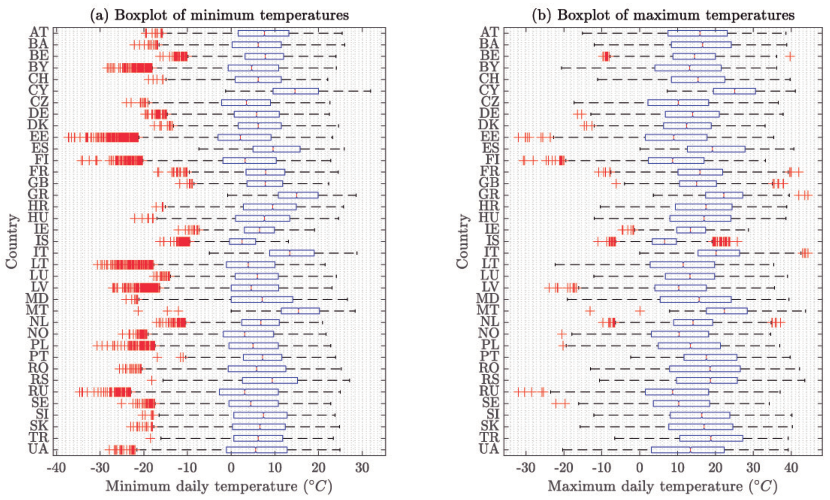
, from January 1980 to December 2019. Thus, this case study consists of 74 daily time series of length 40 years (14,610 days). Furthermore, let us describe the different data partitions that have been used in this paper. The years 1980–2009 have been used as training data (in-sample, 10958 points), and years 2010–2019 have been used as test set (out-of-sample, 3652 points). Figure 6 shows the boxplot of the minimum and maximum daily temperatures of the selected station for each country, once main outliers have been removed (see

Table A2. Detail of the outliers removed from the reference weather stations, and TMAX and TMIN time series in the studied interval (January 1980 to December 2019).

Country	Variable	Outliers
		Date	Value (°C)
LV	TMIN	13 March 1997	81.70
	TMAX	29 December 1994	87.20
		12 March 1997	85.70
MD	TMAX	27 January 1995	66.60
MT	TMIN	2 October 1983	78.90
		23 February 1989	71.10
		18 June 1989	78.10
		5 February 1995	89.10
	TMAX	20 February 1988	77.60
		28 January 1990	67.50
		7 December 1990	63.10

). It is noticeable the clear differences between the Mediterranean countries, such as Malta (MT), Italy (IT), Greece (GR), Spain (ES) or Cyprus (CY), and the rest.

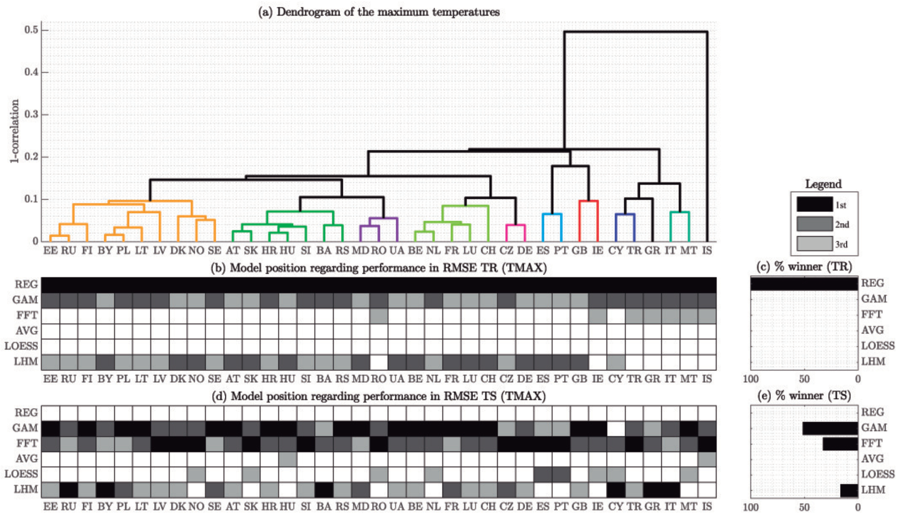
Dendrograms of Figure 7 summarize the complex spatio-temporal correlations of the selected weather stations based on the minimum and maximum temperatures, respectively. It is remarkable that, considering a correlation threshold of 0.9, the clusters formed in both dendrograms are different. For example, according to the dendrogram of TMAX shown in Figure 7a, Finland (FI) has similar maximum temperatures to Norway (NO), Denmark (DK) and Sweden (SE), whereas according to the one of TMIN (bottom), FI is closer to Russia (RU) and Estonia (EE) in terms of minimum temperature.

Figure 8 shows the location of the selected weather stations. Each station has been coloured according to the identified clusters of the dendrogram of the maximum temperature (see Figure 7a). Note that both latitude and longitude explain those clusters.

4.2. Importance of the Trend Component

This section aims to briefly analyze the effect of including the trend in all the methods described in Section 2. To do that, two versions of each model have been fitted, one using linear trends as described in Section 3, and other just using seasonal components and the level (i.e., mean value) of each time series.

Table 2. Out-of-sample (TS) error improvements ($\Delta RMSE$, %) obtained by including linear trends in all the methods, for the minimum and maximum temperatures from the 37 European countries.

Country ID	TMIN—Error Improvement ($\Delta \mathit{R}\mathit{M}\mathit{S}\mathit{E}\mathit{T}\mathit{S}$, %)						TMAX—Error Improvement ($\Delta \mathit{R}\mathit{M}\mathit{S}\mathit{E}\mathit{T}\mathit{S}$, %)
	REG	GAM	FFT	AVG	LOESS	LHM	REG	GAM	FFT	AVG	LOESS	LHM
AT	−4.353	−4.472	−4.507	−4.401	−4.485	−4.327	−3.821	−3.893	−3.923	−3.809	−4.118	−3.895
BA	−3.777	−3.881	−3.889	−3.811	−3.645	−3.915	−2.915	−2.955	−2.984	−2.914	−2.810	−2.965
BE	−1.530	−1.581	−1.638	−1.543	−1.401	−1.578	−1.537	−1.585	−1.620	−1.551	−1.843	−1.548
BY	−1.150	−1.180	−1.204	−1.165	−1.119	−1.176	−2.151	−2.191	−2.208	−2.147	−2.181	−2.278
CH	2.057	2.162	2.044	2.150	2.211	2.174	−1.842	−1.896	−1.911	−1.853	−2.296	−1.847
CY	−15.007	−15.300	−15.425	−15.070	−14.854	−15.312	−7.798	−8.005	−8.158	−7.956	−8.179	−7.985
CZ	−6.971	−7.185	−7.239	−7.112	−7.249	−6.903	−1.758	−1.809	−1.863	−1.776	−2.132	−1.806
DE	−0.439	−0.448	−0.477	−0.431	−0.500	−0.455	−2.051	−2.104	−2.153	−2.083	−2.336	−2.110
DK	−1.161	−1.201	−1.247	−1.170	−1.200	−1.204	−4.440	−4.536	−4.604	−4.407	−4.576	−4.502
EE	1.906	1.952	1.899	2.009	2.534	2.586	−1.709	−1.773	−1.790	−1.727	−1.884	−1.759
ES	−2.929	−3.020	−3.069	−2.927	−3.133	−2.551	−2.481	−2.560	−2.630	−2.508	−2.772	−2.560
FI	−2.929	−3.083	−3.071	−3.030	−2.993	−3.094	−1.937	−2.027	−2.079	−1.892	−2.046	−2.020
FR	−0.716	−0.732	−0.748	−0.705	−0.720	−0.726	−1.933	−1.998	−2.026	−1.953	−2.270	−2.061
GB	−0.079	−0.097	−0.150	−0.075	−0.074	−0.107	−1.560	−1.627	−1.656	−1.589	−1.824	−1.991
GR	−6.680	−6.837	−6.856	−6.878	−6.922	−6.926	−2.559	−2.638	−2.688	−2.620	−2.636	−2.668
HR	−5.897	−6.055	−6.087	−5.942	−6.052	−6.771	−4.622	−4.705	−4.730	−4.587	−4.623	−4.756
HU	−3.746	−3.880	−3.897	−3.784	−3.812	−3.826	−2.219	−2.277	−2.308	−2.272	−2.321	−2.273
IE	−0.448	−0.456	−0.450	−0.452	−0.464	−0.450	5.978	6.086	6.061	6.017	5.985	6.049
IS	−8.999	−9.388	−9.497	−9.427	−9.239	−9.297	−0.250	−0.263	−0.290	−0.225	−0.387	−0.298
IT	−5.217	−5.370	−5.388	−5.326	−5.274	−5.376	−1.034	−1.076	−1.124	−1.054	−1.282	−1.163
LT	−2.666	−2.746	−2.765	−2.686	−2.450	−2.713	−1.629	−1.676	−1.723	−1.600	−1.714	−1.930
LU	−1.504	−1.549	−1.608	−1.491	−1.597	−1.409	−1.953	−2.001	−2.037	−1.946	−2.696	−1.992
LV	−1.551	−1.615	−1.638	−1.554	−1.613	−1.583	−1.325	−1.361	−1.421	−1.309	−1.407	−1.355
MD	−2.888	−3.008	−3.068	−2.896	−2.836	−2.774	−3.225	−3.349	−3.329	−3.235	−3.359	−3.301
MT	−2.620	−2.734	−2.847	−2.542	−2.579	−2.635	−1.256	−1.322	−1.344	−1.319	−1.450	−1.297
NL	0.005	−0.007	−0.045	0.015	0.069	−0.030	−1.372	−1.419	−1.480	−1.383	−1.780	−1.419
NO	0.374	0.367	0.300	0.397	0.529	0.328	−0.795	−0.841	−0.933	−0.818	−1.014	−0.527
PL	−4.342	−4.459	−4.471	−4.248	−4.291	−4.444	−3.660	−3.728	−3.755	−3.668	−3.760	−3.670
PT	−0.647	−0.665	−0.677	−0.666	−0.652	−0.657	−2.766	−2.840	−2.898	−2.802	−3.064	−2.846
RO	−0.562	−0.580	−0.596	−0.615	−0.602	−0.583	−2.012	−2.102	−2.156	−2.051	−1.985	−1.997
RS	−6.853	−7.056	−7.069	−6.916	−7.021	−6.960	−3.194	−3.277	−3.308	−3.245	−3.362	−3.272
RU	−3.413	−3.566	−3.579	−3.534	−3.401	−3.848	−1.424	−1.487	−1.504	−1.436	−1.532	−1.737
SE	−0.742	−0.801	−0.840	−0.732	−1.060	−1.004	−1.649	−1.737	−1.786	−1.671	−1.921	−1.893
SI	−7.528	−7.749	−7.811	−7.669	−7.484	−7.474	−3.870	−3.956	−4.009	−3.939	−4.111	−3.958
SK	−3.432	−3.533	−3.589	−3.461	−3.463	−3.820	−3.213	−3.287	−3.352	−3.251	−3.492	−3.226
TR	−4.612	−4.680	−4.749	−4.585	−4.635	−4.677	−3.892	−4.050	−4.111	−4.035	−3.898	−4.498
UA	−4.147	−4.297	−4.317	−4.152	−3.970	−4.438	−4.484	−4.620	−4.649	−4.368	−4.497	−4.586

shows the out-of-sample error improvements obtained by including the trend in each case, calculated as the percentage improvement in RMSE of the model with linear trend, compared to the one using the mean.

First, it can be seen that results are systematic—the effect of including the trend in a particular time series (minimum or maximum from any country) provides similar error improvements regardless the model in use. Secondly, regarding trend significance, we have obtained p-values lower than 0.05 in 73 of the 74 time series: the only exception is the minimum temperature from Romania (RO), with a p-value of 0.112. Starting from this point, it can be clearly seen that including the trend improves model performance in nearly all the cases. In terms of minimum temperatures, excluding RO, 92% of the countries present out-of-sample error improvements, whereas in the case of TMAX, that rate rises to 97%. Finally, it can be seen that several countries, such as Cyprus (CY), Poland (PL), or Serbia (RS) present high error improvements. However, in the other side, one of the 74 analyzed time series has a surprising result: the trend of the minimum temperature from Ireland (IE), whose p-value is 7.41$·{10}^{-5}$, and providing nearly an 1% of in-sample error improvement, causes an out-of-sample error increase of 6%. As it will be discussed in Section 4.4, for all the models, the resulting trend in the minimum temperature of IE has been negative, and it seems not to be the behavior of the time series during the 10 years of test set. Ignoring that case, and as aforementioned, the trend has proved to improve model out-of-sample performance in most of series and countries.

4.3. Empirical Comparative Analysis

Having described the dataset to be used, and having confirmed the importance of the trend component in long-term temperature forecasting, this section aims to compare the performance of the different candidate models of Table 1 in the selected 37 reference European stations (see Table A1). As aforementioned, for those methods that require selecting model complexity (i.e., FFT, LOESS and AVG), their hyper-parameters have been estimated for each country by using repeated cross-validation, and are detailed in

Table A4. Complexity selected for each country and method, and for minimum and maximum temperatures. From left to right: number of harmonics for the FFT, window size for AVG and LOESS, and number of knots for the LHM.

Country ID	FFT		AVG		LOESS		LHM
	TMIN	TMAX	TMIN	TMAX	TMIN	TMAX	TMIN	TMAX
AT	1	2	117	115	319	283	7	7
BA	1	2	127	109	325	295	5	7
BE	1	2	125	117	323	303	5	7
BY	1	1	133	101	331	261	6	7
CH	1	2	113	103	325	275	7	8
CY	2	2	91	103	279	283	8	9
CZ	1	2	117	105	323	255	7	6
DE	1	2	129	103	327	287	5	7
DK	2	1	117	101	317	251	7	8
EE	1	1	137	105	333	275	8	7
ES	2	2	97	89	231	223	7	11
FI	1	2	125	125	301	309	6	7
FR	2	2	125	107	319	269	5	7
GB	2	2	121	109	313	277	8	7
GR	2	1	99	107	263	321	8	6
HR	1	2	111	107	307	295	7	7
HU	1	2	117	95	317	277	7	8
IE	2	2	121	117	293	289	6	6
IS	2	2	123	169	289	343	6	5
IT	2	2	91	107	259	291	7	8
LT	1	2	139	109	347	261	6	7
LU	1	2	123	111	337	291	7	7
LV	1	2	141	101	347	265	6	6
MD	1	1	115	99	311	281	7	9
MT	2	2	105	87	303	241	6	6
NL	2	1	137	119	343	323	5	6
NO	1	1	117	107	319	291	5	8
PL	1	1	145	107	351	283	7	7
PT	2	2	115	87	301	237	6	10
RO	1	2	115	105	311	287	7	9
RS	1	2	109	99	311	273	7	8
RU	1	1	109	99	295	285	7	8
SE	2	2	121	99	317	265	7	6
SI	1	2	105	91	321	275	7	7
SK	1	2	127	99	329	249	6	8
TR	3	2	95	99	241	271	8	8
UA	1	2	129	111	315	279	8	9

. The estimated number of knots of the LHM for each country, which is automatically determined by its learning algorithm, can be also seen in Table A4. The results provided by the six methods over the 37 reference weather stations, and for their minimum and maximum temperatures, are detailed below.

First, before presenting the R-squared and the in-sample and out-of-sample errors (RMSE) of all the methods, Figure 9 and Figure 10 show the relative position of the different methods when estimating the minimum and maximum temperatures, respectively, and in-sample and out-of-sample. It should be noted that in both figures, countries have been sorted attending to the clusters of Figure 7 but there is not a best performing model for each group, and we have not found any relationship between that ordering and model performance.

The results obtained for the minimum and maximum temperatures are quite similar—the best performing models are the same in Figure 9 and Figure 10. First, it should be noted that regarding in-sample error, the REG method outperforms in all the countries all the other models. However, it can be seen that REG is never selected as one of the the top-3 models for out-of-sample performance. For that reason, we can conclude that it is clearly over-fitted. Ignoring REG, it can be seen that in both minimum and maximum temperatures, the second and third places regarding in-sample error belong to the GAM, and the LHM (the latter, beaten by the FFT in some countries).

On the other hand, in the out-of-sample set, there are three models that clearly outperform the others—GAM, FFT an LHM. The first one, that also was the second best in-sample performer after the over-fitted REG, has the lowest out-of-sample RMSE in most of the cases. As it can be seen in Figure 9 and Figure 10, GAM is the out-of-sample winner in almost 60% of the countries, both in the minimum and maximum temperatures. After the GAM, FFT provides the lowest error in approximately 25% of the countries, and LHM in the vast majority of remaining cases.

Before presenting the RMSE for all the methods and countries, and in order to check the goodness of the estimated deterministic (trend plus seasonal) components explaining temperature variance,

Table 3. Summary of the in-sample (TR) and out-of-sample (TS) Adjusted R-squared ($R_{adj}^2$) for the minimum temperatures, obtained with all the different methods and for all the countries. The bold values with * indicate the best method for each country and dataset.

Country ID	${\mathit{R}}_{\mathit{a}\mathit{d}\mathit{j}}^2$ (TMIN–TR)						${\mathit{R}}_{\mathit{a}\mathit{d}\mathit{j}}^2$ (TMIN–TS)
	REG	GAM	FFT	AVG	LOESS	LHM	REG	GAM	FFT	AVG	LOESS	LHM
AT	0.777 *	0.772	0.771	0.768	0.768	0.772	0.779	0.785	0.785 *	0.780	0.781	0.785
BA	0.721 *	0.713	0.711	0.708	0.709	0.712	0.717	0.725	0.724	0.719	0.720	0.728 *
BE	0.660 *	0.650	0.647	0.646	0.646	0.648	0.619	0.630 *	0.628	0.627	0.626	0.624
BY	0.709 *	0.703	0.702	0.697	0.698	0.701	0.683	0.691 *	0.689	0.686	0.687	0.689
CH	0.767 *	0.761	0.758	0.757	0.756	0.761	0.760	0.770 *	0.768	0.762	0.761	0.768
CY	0.850 *	0.845	0.845	0.844	0.844	0.845	0.860	0.863	0.863 *	0.861	0.861	0.863
CZ	0.740 *	0.734	0.732	0.730	0.729	0.734	0.717	0.725	0.726 *	0.721	0.722	0.722
DE	0.709 *	0.702	0.700	0.696	0.697	0.700	0.700	0.706 *	0.704	0.699	0.701	0.705
DK	0.777 *	0.770	0.770	0.766	0.765	0.770	0.763	0.771	0.772 *	0.769	0.770	0.772
EE	0.705 *	0.696	0.693	0.688	0.689	0.698	0.666	0.680 *	0.677	0.674	0.672	0.675
ES	0.812 *	0.807	0.805	0.804	0.805	0.806	0.822	0.828	0.828 *	0.822	0.827	0.825
FI	0.741 *	0.735	0.731	0.729	0.731	0.733	0.741	0.753 *	0.749	0.749	0.750	0.751
FR	0.656 *	0.647	0.647	0.642	0.643	0.643	0.641	0.647 *	0.646	0.641	0.642	0.639
GB	0.660 *	0.651	0.651	0.647	0.647	0.652	0.633	0.643 *	0.642	0.638	0.639	0.640
GR	0.816 *	0.810	0.808	0.807	0.807	0.808	0.785	0.791	0.789	0.790	0.789	0.792 *
HR	0.794 *	0.788	0.786	0.785	0.785	0.789	0.790	0.796 *	0.795	0.792	0.792	0.796
HU	0.779 *	0.773	0.772	0.769	0.770	0.773	0.787	0.795 *	0.794	0.789	0.790	0.792
IE	0.583 *	0.571	0.571	0.567	0.568	0.569	0.491	0.500 *	0.500	0.496	0.497	0.495
IS	0.598 *	0.587	0.585	0.581	0.580	0.585	0.572	0.591	0.594 *	0.593	0.587	0.588
IT	0.824 *	0.818	0.818	0.817	0.816	0.818	0.809	0.815	0.813	0.812	0.811	0.815 *
LT	0.699 *	0.692	0.690	0.685	0.685	0.692	0.686	0.694 *	0.691	0.685	0.686	0.690
LU	0.707 *	0.699	0.697	0.695	0.694	0.699	0.688	0.697 *	0.697	0.692	0.692	0.693
LV	0.710 *	0.703	0.699	0.695	0.695	0.700	0.695	0.707 *	0.704	0.695	0.697	0.701
MD	0.805 *	0.799	0.799	0.795	0.796	0.799	0.792	0.801	0.801 *	0.794	0.796	0.798
MT	0.799 *	0.792	0.792	0.789	0.789	0.791	0.839	0.846 *	0.845	0.838	0.839	0.843
NL	0.615 *	0.603	0.603	0.597	0.597	0.600	0.602	0.614 *	0.613	0.605	0.606	0.608
NO	0.763 *	0.756	0.753	0.752	0.751	0.755	0.746	0.761 *	0.759	0.756	0.756	0.758
PL	0.707 *	0.701	0.700	0.692	0.695	0.701	0.723	0.730 *	0.729	0.714	0.718	0.729
PT	0.685 *	0.677	0.675	0.672	0.671	0.673	0.622	0.632	0.632	0.634 *	0.633	0.626
RO	0.787 *	0.781	0.780	0.777	0.777	0.781	0.766	0.774 *	0.772	0.768	0.768	0.772
RS	0.770 *	0.764	0.762	0.761	0.760	0.764	0.765	0.772 *	0.771	0.767	0.767	0.769
RU	0.760 *	0.754	0.752	0.751	0.750	0.753	0.758	0.768 *	0.766	0.765	0.766	0.766
SE	0.779 *	0.772	0.772	0.767	0.767	0.773	0.767	0.779 *	0.778	0.774	0.775	0.775
SI	0.778 *	0.772	0.771	0.770	0.769	0.772	0.780	0.787 *	0.787	0.785	0.784	0.785
SK	0.746 *	0.739	0.738	0.734	0.735	0.739	0.737	0.745	0.745 *	0.740	0.741	0.745
TR	0.771 *	0.764	0.764	0.762	0.762	0.764	0.769	0.772	0.773 *	0.769	0.769	0.772
UA	0.787 *	0.782	0.780	0.775	0.777	0.782	0.786	0.793 *	0.791	0.784	0.787	0.791

and

Table 4. Summary of the in-sample (TR) and out-of-sample (TS) Adjusted R-squared ($R_{adj}^2$) for the maximum temperatures, obtained with all the different methods and for all the countries. The bold values with * indicate the best method for each country and dataset.

Country ID	${\mathit{R}}_{\mathit{a}\mathit{d}\mathit{j}}^2$ (TMAX–TR)						${\mathit{R}}_{\mathit{a}\mathit{d}\mathit{j}}^2$ (TMAX–TS)
	REG	GAM	FFT	AVG	LOESS	LHM	REG	GAM	FFT	AVG	LOESS	LHM
AT	0.788 *	0.782	0.781	0.778	0.779	0.783	0.776	0.780 *	0.780	0.775	0.777	0.779
BA	0.731 *	0.723	0.722	0.720	0.719	0.722	0.720	0.725	0.725	0.719	0.718	0.727 *
BE	0.718 *	0.711	0.710	0.707	0.707	0.713	0.699	0.707 *	0.707	0.701	0.703	0.705
BY	0.805 *	0.800	0.795	0.797	0.796	0.800	0.796	0.799	0.797	0.795	0.797	0.800 *
CH	0.786 *	0.780	0.780	0.778	0.777	0.781	0.773	0.779 *	0.777	0.775	0.775	0.776
CY	0.874 *	0.871	0.870	0.868	0.869	0.871	0.870	0.873	0.874	0.873	0.873	0.874 *
CZ	0.756 *	0.749	0.746	0.746	0.745	0.748	0.737	0.744	0.744 *	0.739	0.743	0.744
DE	0.767 *	0.761	0.758	0.758	0.756	0.761	0.748	0.754	0.755 *	0.751	0.753	0.754
DK	0.817 *	0.813	0.808	0.810	0.809	0.813	0.820	0.824	0.824 *	0.819	0.822	0.823
EE	0.809 *	0.804	0.800	0.801	0.800	0.803	0.806	0.812 *	0.810	0.808	0.809	0.810
ES	0.829 *	0.824	0.821	0.821	0.820	0.825	0.825	0.831	0.831 *	0.826	0.831	0.829
FI	0.831 *	0.827	0.825	0.821	0.821	0.827	0.830	0.837 *	0.836	0.828	0.830	0.834
FR	0.746 *	0.739	0.739	0.737	0.737	0.740	0.734	0.742 *	0.741	0.737	0.739	0.741
GB	0.746 *	0.740	0.739	0.737	0.737	0.740	0.723	0.732 *	0.731	0.727	0.729	0.730
GR	0.760 *	0.752	0.751	0.749	0.749	0.750	0.752	0.760	0.761	0.759	0.759	0.762 *
HR	0.787 *	0.781	0.781	0.778	0.778	0.781	0.777	0.782 *	0.780	0.776	0.777	0.780
HU	0.788 *	0.781	0.781	0.780	0.778	0.782	0.771	0.777 *	0.777	0.776	0.776	0.776
IE	0.728 *	0.722	0.722	0.718	0.719	0.721	0.665	0.672 *	0.672	0.666	0.670	0.667
IS	0.446 *	0.431	0.430	0.416	0.417	0.422	0.413	0.440	0.443 *	0.439	0.438	0.428
IT	0.828 *	0.823	0.823	0.820	0.820	0.823	0.814	0.821	0.821	0.820	0.820	0.822 *
LT	0.821 *	0.816	0.815	0.812	0.811	0.815	0.815	0.819 *	0.819	0.812	0.816	0.819
LU	0.750 *	0.744	0.743	0.740	0.740	0.744	0.737	0.743 *	0.742	0.737	0.740	0.741
LV	0.793 *	0.787	0.785	0.784	0.782	0.787	0.793	0.798	0.799 *	0.792	0.794	0.797
MD	0.808 *	0.802	0.799	0.800	0.799	0.803	0.803	0.810 *	0.806	0.804	0.805	0.809
MT	0.864 *	0.859	0.858	0.858	0.857	0.857	0.870	0.877 *	0.876	0.875	0.875	0.874
NL	0.732 *	0.725	0.721	0.721	0.719	0.723	0.712	0.720 *	0.720	0.715	0.717	0.715
NO	0.826 *	0.821	0.818	0.818	0.817	0.821	0.812	0.820	0.822 *	0.817	0.819	0.818
PL	0.794 *	0.789	0.785	0.785	0.784	0.788	0.783	0.786 *	0.785	0.782	0.784	0.786
PT	0.763 *	0.756	0.753	0.754	0.752	0.757	0.770	0.776	0.778 *	0.773	0.776	0.775
RO	0.822 *	0.817	0.816	0.814	0.814	0.816	0.811	0.819	0.820 *	0.815	0.815	0.815
RS	0.744 *	0.737	0.736	0.735	0.734	0.737	0.734	0.741 *	0.741	0.738	0.738	0.740
RU	0.818 *	0.814	0.811	0.811	0.810	0.814	0.817	0.824	0.821	0.819	0.819	0.824 *
SE	0.824 *	0.819	0.817	0.816	0.816	0.819	0.827	0.834 *	0.832	0.829	0.831	0.833
SI	0.810 *	0.804	0.804	0.803	0.801	0.804	0.789	0.794	0.794 *	0.793	0.793	0.793
SK	0.813 *	0.808	0.807	0.805	0.806	0.808	0.793	0.798	0.799 *	0.796	0.798	0.797
TR	0.839 *	0.835	0.835	0.833	0.833	0.834	0.836	0.843	0.843 *	0.841	0.841	0.842
UA	0.825 *	0.821	0.818	0.816	0.816	0.821	0.819	0.825 *	0.824	0.814	0.818	0.823

present the Adjusted R-squared ($R_{adj}^2$) for the minimum and maximum temperatures, respectively. It can be seen that, in spite of the fact that the remainder has not been modelled and, therefore, forecasting performance can be improved, the obtained $R_{adj}^2$ are over 0.7 in the vast majority of cases. The average $R_{adj}^2$ for the minimum temperature and all the models and countries is of 0.731, for both in-sample and out-of-sample sets. Regarding maximum temperature, the average $R_{adj}^2$ is 0.777 and 0.776 respectively. The only cases where a weak $R_{adj}^2$ has been obtained (lower than 0.5 in average) are Ireland (IE), for its out-of-sample minimum temperature, and Iceland (IS), for its maximum temperature (both in- and out-of-sample).

Finally,

Table 5. Summary of the in-sample (TR) and out-of-sample (TS) errors for the minimum temperatures, obtained with all the different methods and for all the countries. The bold values with * indicate the best method for each country and dataset.

Country ID	RMSE (TMIN–TR)						RMSE (TMIN–TS)
	REG	GAM	FFT	AVG	LOESS	LHM	REG	GAM	FFT	AVG	LOESS	LHM
AT	3.436 *	3.477	3.488	3.507	3.505	3.478	3.428	3.380	3.376 *	3.415	3.406	3.378
BA	3.830 *	3.885	3.895	3.919	3.912	3.889	3.850	3.793	3.806	3.836	3.831	3.779 *
BE	3.429 *	3.476	3.490	3.498	3.496	3.488	3.574	3.524 *	3.535	3.540	3.539	3.551
BY	4.373 *	4.419	4.428	4.465	4.454	4.433	4.553	4.499 *	4.513	4.533	4.526	4.512
CH	3.111 *	3.156	3.173	3.180	3.186	3.155	3.206	3.141 *	3.151	3.194	3.197	3.151
CY	2.329 *	2.362	2.365	2.374	2.376	2.362	2.243	2.221	2.219 *	2.239	2.235	2.220
CZ	3.712 *	3.761	3.775	3.788	3.793	3.761	3.927	3.867	3.860 *	3.894	3.889	3.887
DE	3.608 *	3.651	3.665	3.685	3.679	3.662	3.705	3.669 *	3.679	3.711	3.703	3.676
DK	2.966 *	3.008	3.014	3.037	3.041	3.008	3.022	2.972	2.965 *	2.985	2.980	2.966
EE	4.924 *	4.993	5.020	5.056	5.048	4.981	5.122	5.014 *	5.039	5.062	5.060	5.058
ES	2.801 *	2.836	2.853	2.858	2.856	2.844	2.858	2.813	2.813 *	2.860	2.820	2.836
FI	4.424 *	4.477	4.513	4.524	4.511	4.497	4.342	4.240 *	4.275	4.280	4.267	4.261
FR	3.469 *	3.512	3.514	3.535	3.533	3.532	3.556	3.524 *	3.532	3.555	3.550	3.562
GB	3.103 *	3.143	3.144	3.162	3.163	3.139	3.188	3.146 *	3.152	3.166	3.162	3.157
GR	2.336 *	2.374	2.383	2.390	2.391	2.383	2.507	2.477	2.484	2.481	2.483	2.467 *
HR	3.376 *	3.420	3.437	3.446	3.446	3.418	3.422	3.372 *	3.380	3.407	3.405	3.375
HU	3.612 *	3.656	3.669	3.687	3.684	3.654	3.560	3.494 *	3.502	3.544	3.535	3.521
IE	2.886 *	2.927	2.927	2.941	2.939	2.934	3.401	3.369 *	3.371	3.382	3.380	3.385
IS	2.697 *	2.736	2.740	2.755	2.757	2.740	2.544	2.486	2.479 *	2.481	2.497	2.497
IT	2.570 *	2.611	2.615	2.621	2.625	2.612	2.707	2.666	2.674	2.683	2.689	2.666 *
LT	4.445 *	4.493	4.507	4.547	4.543	4.498	4.583	4.519 *	4.541	4.586	4.584	4.551
LU	3.471 *	3.516	3.529	3.542	3.548	3.518	3.555	3.504 *	3.509	3.534	3.537	3.532
LV	4.057 *	4.104	4.135	4.161	4.158	4.124	4.284	4.204 *	4.220	4.285	4.274	4.246
MD	3.863 *	3.917	3.923	3.954	3.949	3.917	4.073	3.991	3.991 *	4.053	4.040	4.014
MT	2.347 *	2.386	2.388	2.402	2.406	2.394	2.111	2.066 *	2.070	2.113	2.111	2.084
NL	3.574 *	3.626	3.627	3.654	3.654	3.642	3.635	3.580 *	3.583	3.620	3.616	3.604
NO	3.740 *	3.802	3.820	3.833	3.834	3.807	3.848	3.738 *	3.747	3.772	3.768	3.755
PL	4.170 *	4.214	4.222	4.274	4.257	4.217	4.213	4.159 *	4.168	4.285	4.256	4.171
PT	3.307 *	3.350	3.358	3.372	3.379	3.371	3.563	3.513	3.514	3.506 *	3.509	3.543
RO	3.789 *	3.846	3.853	3.879	3.874	3.842	4.062	3.994 *	4.006	4.046	4.041	4.010
RS	3.716 *	3.765	3.776	3.787	3.789	3.760	3.830	3.771 *	3.782	3.815	3.814	3.797
RU	4.602 *	4.663	4.685	4.695	4.699	4.670	4.567	4.473 *	4.495	4.500	4.498	4.489
SE	3.488 *	3.540	3.546	3.579	3.582	3.536	3.544	3.456 *	3.460	3.495	3.491	3.484
SI	3.495 *	3.539	3.548	3.558	3.567	3.542	3.421	3.366 *	3.368	3.384	3.391	3.381
SK	3.890 *	3.938	3.945	3.978	3.971	3.944	3.934	3.875	3.873 *	3.915	3.905	3.876
TR	3.379 *	3.428	3.430	3.443	3.445	3.428	3.398	3.376	3.373 *	3.401	3.396	3.376
UA	4.189 *	4.239	4.257	4.300	4.285	4.233	4.271	4.194 *	4.219	4.287	4.262	4.219

and

Table 6. Summary of the in-sample (TR) and out-of-sample (TS) errors for the maximum temperatures, obtained with all the different methods and for all the countries. The bold values with * indicate the best method for each country and dataset.

Country ID	RMSE (TMAX–TR)						RMSE (TMAX–TS)
	REG	GAM	FFT	AVG	LOESS	LHM	REG	GAM	FFT	AVG	LOESS	LHM
AT	4.391 *	4.448	4.461	4.492	4.485	4.445	4.610	4.567 *	4.573	4.624	4.603	4.576
BA	5.163 *	5.240	5.245	5.268	5.277	5.244	5.421	5.376	5.374	5.431	5.440	5.360 *
BE	3.924 *	3.973	3.981	4.001	4.003	3.965	4.152	4.094 *	4.095	4.135	4.125	4.110
BY	4.529 *	4.586	4.638	4.618	4.629	4.584	4.790	4.753	4.780	4.804	4.784	4.744 *
CH	4.065 *	4.122	4.128	4.146	4.151	4.120	4.216	4.151 *	4.174	4.191	4.192	4.182
CY	2.250 *	2.276	2.284	2.301	2.298	2.281	2.224	2.195	2.189	2.196	2.196	2.187 *
CZ	4.729 *	4.797	4.825	4.826	4.833	4.806	5.144	5.077	5.072 *	5.125	5.092	5.073
DE	4.320 *	4.373	4.399	4.400	4.417	4.369	4.593	4.541	4.529 *	4.564	4.551	4.545
DK	3.276 *	3.314	3.351	3.340	3.344	3.311	3.371	3.336	3.335 *	3.384	3.356	3.344
EE	4.415 *	4.472	4.518	4.512	4.518	4.481	4.532	4.459 *	4.484	4.512	4.494	4.485
ES	3.551 *	3.603	3.633	3.627	3.637	3.591	3.814	3.755	3.745 *	3.805	3.745	3.769
FI	3.728 *	3.772	3.794	3.844	3.837	3.782	3.803	3.731 *	3.744	3.831	3.806	3.762
FR	3.920 *	3.972	3.976	3.994	3.993	3.968	4.052	3.988 *	4.001	4.027	4.017	3.995
GB	3.275 *	3.313	3.318	3.334	3.333	3.310	3.497	3.438 *	3.447	3.472	3.459	3.453
GR	2.895 *	2.941	2.946	2.957	2.961	2.954	2.881	2.836	2.828	2.840	2.840	2.821 *
HR	4.299 *	4.357	4.362	4.387	4.390	4.360	4.518	4.472 *	4.487	4.530	4.524	4.491
HU	4.584 *	4.649	4.658	4.669	4.683	4.646	4.742	4.676 *	4.678	4.686	4.689	4.692
IE	2.579 *	2.609	2.610	2.629	2.624	2.614	2.932	2.900 *	2.901	2.927	2.914	2.924
IS	3.425 *	3.471	3.475	3.517	3.513	3.500	3.107	3.034	3.026 *	3.035	3.042	3.067
IT	2.769 *	2.810	2.811	2.835	2.833	2.812	2.814	2.759	2.759	2.767	2.768	2.753 *
LT	4.240 *	4.295	4.311	4.344	4.348	4.305	4.503	4.452 *	4.455	4.543	4.499	4.459
LU	4.164 *	4.218	4.226	4.245	4.249	4.215	4.386	4.332 *	4.339	4.383	4.372	4.350
LV	3.858 *	3.915	3.927	3.943	3.960	3.918	4.015	3.971	3.961 *	4.025	4.006	3.983
MD	4.775 *	4.843	4.887	4.870	4.878	4.837	5.104	5.008 *	5.062	5.095	5.085	5.031
MT	2.351 *	2.392	2.399	2.402	2.406	2.406	2.279	2.216 *	2.224	2.231	2.228	2.235
NL	3.591 *	3.637	3.664	3.666	3.675	3.650	3.766	3.713 *	3.715	3.744	3.742	3.745
NO	3.823 *	3.882	3.911	3.917	3.918	3.879	4.017	3.930	3.907 *	3.965	3.943	3.958
PL	4.448 *	4.507	4.553	4.544	4.557	4.518	4.708	4.668 *	4.677	4.712	4.696	4.669
PT	4.002 *	4.062	4.086	4.080	4.098	4.057	4.117	4.065	4.045 *	4.092	4.061	4.071
RO	4.609 *	4.673	4.676	4.712	4.712	4.680	4.783	4.682	4.672 *	4.732	4.727	4.733
RS	5.100 *	5.174	5.179	5.194	5.197	5.175	5.266	5.194 *	5.197	5.225	5.224	5.206
RU	4.420 *	4.472	4.511	4.504	4.516	4.475	4.528	4.447	4.482	4.504	4.506	4.442 *
SE	3.784 *	3.842	3.864	3.868	3.876	3.844	3.811	3.731 *	3.744	3.778	3.764	3.736
SI	4.163 *	4.228	4.234	4.242	4.262	4.228	4.465	4.409	4.408 *	4.423	4.419	4.416
SK	4.365 *	4.423	4.433	4.451	4.448	4.422	4.639	4.583	4.574 *	4.608	4.590	4.600
TR	3.845 *	3.898	3.901	3.926	3.919	3.906	3.817	3.740	3.734 *	3.756	3.757	3.748
UA	4.533 *	4.593	4.622	4.649	4.657	4.585	4.971	4.898 *	4.911	5.045	4.996	4.915

present the in-sample and out-of-sample errors (RMSE) of all the models, for the minimum and maximum temperatures respectively. As aforementioned, the GAM provides good in-sample results, is always in the top-3 models in terms of out-of sample performance, and beating all the others in almost 60% of cases. For that reason, in order to analyze long-term temperature trends in Europe, and their expected values in the following years Section 4.4, the GAM will be the only method to use.

4.4. Analysis of the Long-Term Temperature Trends with the Best Performance Model

Once analysed the performance of all the different methods over the 37 European countries, and confirmed that the GAM is the model, this subsection aims to analyze the results provided by that model in all the countries to shed some light on potential future changes and better understand the behavior of European temperature trends. Furthermore, in order to exhaustively present the results of the GAM, Appendix C presents the seasonal and trend components estimated by this method in all the countries. It should be noted that in spite of the fact that we will only analyze the results provided by the GAM in this section, we could extract the same conclusions, regarding the trend component, with all the tested methods, since their resulting trends are very similar. As an example, the average difference between the three best performing models (FFT, LHM and GAM) in the trends of the minimum temperatures is 9.43$·{10}^{-4}$ °C/year.

It should be noted that this section presents the resulting trends of the GAM, using the reference weather stations from the ECA&D dataset presented in Table A1. Although we have performed a systematic data pre-processing step, removing outliers and filling all the missing points (see Appendix A), any data inconsistency in the original dataset can affect model results. As an example, the reference weather station from Estonia, presents a sudden temperature increase of around 1 °C during the last 13 years of our in-sample period for its minimum temperature. For that reason, its estimated trend may not be reflecting the actual behavior of that temperature.

Figure 11 shows the trends estimated by the GAM for the minimum and maximum temperatures and all the countries. First, it can be seen that most countries present positive temperature trends in both series, 0.02 to 0.08 °C/year. The only exceptions are Romania (RO), Ireland (IE) and Estonia (EE), regarding TMIN, and Malta (MT) and Croatia (HR) regarding TMAX. In the case of RO, its minimum temperature grows at a rate of 0.007 whereas its maximum does so at 0.06 °C/year. The case of IE is more surprising: although its maximum temperature is growing 0.04 °C each year, is the only country in which the GAM (and all the other models) has estimated a negative trend: its minimum temperature is decreasing 0.013 °C/year. At the far end, EE presents a very similar trend of TMAX to that of IE, but it is the country where the minimum temperature presents a higher growing rate: 0.102 °C/year. However, due to the aforementioned data issue, this result may be not representative.

On the other hand, in terms of maximum temperatures, Malta (MT) is growing slower than all the other countries (0.013 °C/year), and Croatia (HR), just in the other side, has the largest increases with 0.089 °C/year. In summary, the average temperature increase of the minimum temperatures of the 37 European countries is 0.0485 °C/year, whereas the average trend for the maximum temperatures is 0.0554 °C/year. To observe all the detail,

Table 7. Trends (°C/year) for the minimum and maximum temperatures and all the countries, estimated by the GAM model.

Country ID	Trend (°C/Year)		Country ID	Trend (°C/Year)
	TMIN	TMAX		TMIN	TMAX
AT	0.039	0.053	IT	0.031	0.030
BA	0.045	0.046	LT	0.046	0.059
BE	0.065	0.054	LU	0.067	0.079
BY	0.035	0.050	LV	0.042	0.054
CH	0.064	0.056	MD	0.069	0.073
CY	0.065	0.055	MT	0.054	0.013
CZ	0.061	0.076	NL	0.046	0.059
DE	0.029	0.062	NO	0.062	0.069
DK	0.037	0.057	PL	0.041	0.056
EE	0.102	0.047	PT	0.021	0.037
ES	0.033	0.024	RO	0.007	0.061
FI	0.052	0.063	RS	0.061	0.064
FR	0.039	0.061	RU	0.055	0.055
GB	0.056	0.051	SE	0.064	0.072
GR	0.027	0.037	SI	0.071	0.069
HR	0.058	0.089	SK	0.057	0.074
HU	0.042	0.050	TR	0.076	0.042
IE	−0.013	0.041	UA	0.047	0.069
IS	0.046	0.044	-	-	-

shows the results of the GAM in all the different countries and for the minimum and maximum temperatures.

In order to find possible similar behaviors between countries, Figure 12 presents the trends of Table 7, separated in minimum and maximum, and coloured according to the clusters formed shown in Figure 7. First, it can be seen that, once the countries have been sorted by cluster, several trend patterns can be appreciated.

Let us analyze several examples. Cluster number 5 of of maximum temperatures, formed by Baltic countries, Nordic countries (except Iceland), Belarus (BY), Poland (PL) and Russia (RU) presents trend values between 0.047 and 0.072 °C/year. Spain (ES) and Portugal (PT) form, for both minimum and maximum temperatures, the Iberian cluster with positive but low values of trend. Ireland (IE) is in the same cluster than the UK for the maximum temperatures and with similar values; however, they are in two separated clusters for TMIN (IE is the only country with negative trend for that variable). France (FR), Belgium (BE), Switzerland (CH) and the Netherlands (NL) have similar results in terms of maximum temperature, but regarding TMIN FR presents lower increases than all the other neighbours. Italy (IT) and Malta (MT) behaves similarly in TMAX (flat trends), but in TMIN, MT presents a higher value.

In order to check the geographical distribution of these trends, Figure 13 shows the European map of minimum and maximum temperature trends. First, it can be seen that, in general terms, the minimum temperatures are increasing at a slower rhythm than maximum temperatures: 68% of countries present higher growing rates in its maximum temperature. Regarding maximum temperatures, fourteen countries present annual increases higher than 0.06 °C/year, leaded by Croatia (HR) with 0.089 °C/year. Only seven countries grow in minimum and maximum temperatures at a rate higher than 0.06 °C/year—the Czech Republic (CZ), Luxembourg (LU), Moldova (MD), Norway (NO), Serbia (RS), Sweden (SE) and Slovenia (SI). It should be noted that, Finland (FI) with trends of 0.052 and 0.063 °C/year for its minimum and maximum temperatures respectively, is not very far from that group, so Scandinavian countries present quite high grow rates for both variables.

5. Conclusions

Temperature forecasting is a common step for most energy forecasting methods and several techniques for temperature scenario generation can be found in literature. Furthermore, and also related to electric load forecasting, recent papers have discussed the use of temperature trend, concluding that the effect of that component, dealing with two years of training data and one year to test, is negligible in terms of temperature forecasting accuracy.

However, dealing with long-term estimations (i.e., more than three years, and ten years in this paper), and training also with longer time series (40 years), our results have shown that we can make more accurate predictions in the long-term of the daily minimum and maximum temperatures by including a linear trend in the model. Using time series decomposition, and dealing also with the seasonal component, six different methods have been analyzed, concluding that Generalized Additive Models (GAM) outperforms all the others, providing the lowest out-of-sample error in almost 60% of the 74 time series analyzed (minimum and maximum temperatures from reference weather stations from 37 European countries).

In addition, a brief analysis of GAM results for temperatures of those 37 countries has been carried out, showing that both maximum and minimum temperatures present linear increasing trends, (with p-value = 0), and rates between 0.02 and 0.08 °C/year in most cases. As next steps, including the remainder in this kind of temperature decomposition methods will allow us to model the effect of cold and heating waves, and to better understand the behavior and possible correlation, between that component in different countries.

References

1. Feinberg, E.A.; Genethliou, D. Load forecasting. In Applied Mathematics for Restructured Electric Power Systems; Springer: Berlin, Germany, 2005; pp. 269–285. [Google Scholar]
2. Weron, R. Modeling and Forecasting Electricity Loads and Prices: A Statistical Approach; John Wiley and Sons, Ltd.: Hoboken, NJ, USA, 2013. [Google Scholar] [CrossRef]
3. Muñoz, A.; Sánchez-Úbeda, E.F.; Cruz, A.; Marin, J. Short-term Forecasting in Power Systems: A Guided Tour. In Handbook of Power Systems II; Rebennack, S., Pardalos, P.M., Pereira, M.V.F., Iliadis, N.A., Eds.; Energy Systems; Springer: Berlin/Heidelberg, Germany, 2010; pp. 129–160. [Google Scholar] [CrossRef]
4. Hong, T.; Fan, S. Probabilistic electric load forecasting: A tutorial review. Int. J. Forecast. 2016, 32, 914–938. [Google Scholar] [CrossRef]
5. Hong, T.; Pinson, P.; Fan, S. Global Energy Forecasting Competition 2012. Int. J. Forecast. 2014, 30, 357–363. [Google Scholar] [CrossRef]
6. Hong, T.; Pinson, P.; Fan, S.; Zareipour, H.; Troccoli, A.; Hyndman, R.J. Probabilistic energy forecasting: Global Energy Forecasting Competition 2014 and beyond. Int. J. Forecast. 2016, 32, 896–913. [Google Scholar] [CrossRef] [Green Version]
7. Hong, T.; Xie, J.; Black, J. Global energy forecasting competition 2017: Hierarchical probabilistic load forecasting. Int. J. Forecast. 2019. [Google Scholar] [CrossRef]
8. Xie, J.; Hong, T. Temperature Scenario Generation for Probabilistic Load Forecasting. IEEE Trans. Smart Grid 2018, 9, 1680–1687. [Google Scholar] [CrossRef]
9. Hyndman, R.J.; Athanasopoulos, G. Forecasting: Principles and Practice; OTexts: Melbourne, Australia, 2018. [Google Scholar]
10. Cook, J.; Oreskes, N.; Doran, P.T.; Anderegg, W.R.L.; Verheggen, B.; Maibach, E.W.; Carlton, J.S.; Lewandowsky, S.; Skuce, A.G.; Green, S.A.; et al. Consensus on consensus: A synthesis of consensus estimates on human-caused global warming. Environ. Res. Lett. 2016, 11, 048002. [Google Scholar] [CrossRef]
11. Grieser, J.; Trömel, S.; Schönwiese, C.D. Statistical time series decomposition into significant components and application to European temperature. Theor. Appl. Climatol. 2002, 71, 171–183. [Google Scholar] [CrossRef] [Green Version]
12. Sobhani, M.; Hong, T.; Martin, C. Temperature anomaly detection for electric load forecasting. Int. J. Forecast. 2019, 36, 324–333. [Google Scholar] [CrossRef]
13. Guerreiro, S.B.; Dawson, R.J.; Kilsby, C.; Lewis, E.; Ford, A. Future heat-waves, droughts and floods in 571 European cities. Environ. Res. Lett. 2018, 13, 034009. [Google Scholar] [CrossRef]
14. Oppenheim, A.V.; Schafer, R.W.; Buck, J.R. Discrete-Time Signal Processing, 2nd ed.; Prentice-hall Englewood Cliffs: Upper Saddle River, NJ, USA, 1999. [Google Scholar]
15. Hastie, T.; Tibshirani, R. Generalized Additive Models; Wiley Online Library: Hoboken, NJ, USA, 1990. [Google Scholar]
16. Hastie, T.; Tibshirani, R.; Friedman, J. The Elements of Statistical Learning: Data Mining, Inference, and Prediction, 2nd ed.; Springer Science & Business Media: Berlin, Germany, 2009. [Google Scholar]
17. Cleveland, W.S. Robust locally weighted regression and smoothing scatterplots. J. Am. Stat. Assoc. 1979, 74, 829–836. [Google Scholar] [CrossRef]
18. Cleveland, R.B.; Cleveland, W.S.; McRae, J.E.; Terpenning, I. STL: A Seasonal-Trend Decomposition Procedure Based on Loess (with Discussion). J. Off. Stat. 1990, 6, 3–73. [Google Scholar]
19. Sánchez-Úbeda, E.F.; Wehenkel, L. The Hinges model: A one-dimensional continuous piecewise polynomial model. In Proceedings of the International Congress on Information Processing and Management of Uncertainty in Knowledge Based Systems, IPMU98, Paris, France, 6–10 July 1998. [Google Scholar]
20. Sánchez-Úbeda, E.F. Models for Data Analysis: Contributions to Automatic Learning. Ph.D. Thesis, Universidad Pontificia Comillas de Madrid, Madrid, Spain, 1999. [Google Scholar]
21. Wood, S.N. Generalized Additive Models: An Introduction with R, 2nd ed.; CRC Press: Boca Raton, FL, USA, 2017. [Google Scholar]
22. Li, Y.; Jones, B. The Use of Extreme Value Theory for Forecasting Long-Term Substation Maximum Electricity Demand. IEEE Trans. Power Syst. 2019, 35, 128–139. [Google Scholar] [CrossRef]
23. Friedman, J.H.; Stuetzle, W. Projection Pursuit Regression. J. Am. Stat. Assoc. 1981, 76, 817–823. [Google Scholar] [CrossRef]
24. Tibshirani, R. Regression Shrinkage and Selection Via the Lasso. J. R. Stat. Soc. Ser. B (Methodol.) 1996, 58, 267–288. [Google Scholar] [CrossRef]
25. Gascón, A.; Sánchez-Úbeda, E.F. Automatic specification of piecewise linear additive models: Application to forecasting natural gas demand. Stat. Comput. 2018, 28, 201–217. [Google Scholar] [CrossRef]
26. Sánchez-Úbeda, E.F.; Berzosa, A. Modeling and forecasting industrial end-use natural gas consumption. Energy Econ. 2007, 29, 710–742. [Google Scholar] [CrossRef]
27. Friedman, J.; Hastie, T.; Tibshirani, R. Regularization Paths for Generalized Linear Models via Coordinate Descent. J. Stat. Softw. 2010, 33, 1–22. [Google Scholar] [CrossRef] [Green Version]
28. Wright, S.J. Coordinate descent algorithms. Math. Program. 2015, 151, 3–34. [Google Scholar] [CrossRef]
29. Kuhn, M.; Johnson, K. Applied Predictive Modeling; Springer Science & Business Media: Berlin, Germany, 2013. [Google Scholar]
30. Klein Tank, A.M.G.; Wijngaard, J.B.; Können, G.P.; Böhm, R.; Demarée, G.; Gocheva, A.; Mileta, M.; Pashiardis, S.; Hejkrlik, L.; Kern-Hansen, C.; et al. Daily dataset of 20th-century surface air temperature and precipitation series for the European Climate Assessment. Int. J. Climatol. 2002, 22, 1441–1453. [Google Scholar] [CrossRef]
31. Moreno-Carbonell, S.; Sánchez-Úbeda, E.F.; Muñoz, A. Rethinking weather station selection for electric load forecasting using genetic algorithms. Int. J. Forecast. 2019, 36, 695–712. [Google Scholar] [CrossRef]
32. Hong, T.; Wang, P.; White, L. Weather station selection for electric load forecasting. Int. J. Forecast. 2015, 31, 286–295. [Google Scholar] [CrossRef]
Figure 1. Minimum and maximum daily temperatures of four weather stations from Europe: (a) Spain (ES). (b) France (FR). (c) Germany (DE). (d) Sweden (SE).
Energies 13 01569 g001
Figure 2. Seasonal plots where the daily data from each year are overlapped: (a) Spain (ES). (b) France (FR). (c) Germany (DE). (d) Sweden (SE).
Energies 13 01569 g002
Figure 3. Seasonal component for the maximum temperature of Spain. (a) Estimated by all the proposed methods of Table 1. (b) Estimated by REG. (c) Estimated by FFT. (d) Estimated by AVG. (e) Estimated by LOESS. (f) Estimated by LHM. (g) Estimated by GAM. (bg) Black lines in background represent the seasonal components estimated by all the rest of the models of Table 1.
Energies 13 01569 g003
Figure 4. Trend and seasonal components estimated by the FFT model for (a) Spain (ES), and (c) Sweden (SE). (b) and (d) show the detail of the seasonal component estimated for each country. In order to facilitate the comparison between both countries, seasonal components of (b) Sweden and (d) Spain are indicated with red broken lines.
Energies 13 01569 g004
Figure 5. Detail of the error curve with error bars obtained by repeated cross-validation at each point, for the method AVG, and the maximum temperature of Spain. The smoothest model (banwidth = 89) whose error is inside the 95% confidence interval of the best one (banwidth = 61) is chosen, indicated by the red vertical broken line.
Energies 13 01569 g005
Figure 6. Boxplots for the (a) minimum daily temperature and (b) maximum daily temperature of each European country.
Energies 13 01569 g006
Figure 7. Dendrograms of the 37 European weather stations, based on the (a) minimum and (b) maximum temperatures. The coloured clusters correspond to those formed using a correlation threshold of 0.9.
Energies 13 01569 g007
Figure 8. Location of the reference weather stations. The coloured clusters correspond to those formed using the dendrogram of Figure 7a, based on the maximum temperature.
Energies 13 01569 g008
Figure 9. Results for the minimum temperatures and all the tested methods: (a) dendrogram of the 37 weather stations, first three methods with lower (b) in-sample and (d) out-of-sample error, and percentage of times winner for each method: (c) in-sample and (e) out-of-sample.
Energies 13 01569 g009
Figure 10. Results for the maximum temperatures and all the tested methods: (a) dendrogram of the 37 weather stations, first three methods with lower (b) in-sample and (d) out-of-sample error, and percentage of times winner for each method: (c) in-sample and (e) out-of-sample.
Energies 13 01569 g010
Figure 11. Scatterplot of the trends of the minimum and maximum temperatures. Each point represents a country, and colors indicate the cluster to which each point belongs according to Figure 7b. The black broken line represents the values of equal trend for minimum and maximum temperatures.
Energies 13 01569 g011
Figure 12. Trend determined by the GAM for the (a) minimum and (b) maximum temperatures of the 37 countries. The colors indicate the cluster to which each country belongs according to Figure 7.
Energies 13 01569 g012
Figure 13. Annual increase of temperatures obtained from the trend component of the GAM for the (a) minimum and (b) maximum temperatures of the 37 countries.
Energies 13 01569 g013