Abstract
Electromechanical coupling devices have been playing an indispensable role in modern engineering. Particularly, flexoelectricity, an electromechanical coupling effect that involves strain gradients, has shown promising potential for future miniaturized electromechanical coupling devices. Therefore, simulation of flexoelectricity is necessary and inevitable. In this paper, we provide an overview of numerical procedures on modeling flexoelectricity. Specifically, we summarize a generalized formulation including the electrostatic stress tensor, which can be simplified to retrieve other formulations from the literature. We further show the weak and discretization forms of the boundary value problem for different numerical methods, including isogeometric analysis and mixed FEM. Several benchmark problems are presented to demonstrate the numerical implementation. The source code for the implementation can be utilized to analyze and develop more complex flexoelectric nano-devices.
1. Introduction
In recent years, huge attention in various research areas, such as material science, mechanical engineering and chemistry, has been paid to flexoelectricity [1,2], an electromechanical coupling phenomenon in all dielectric materials (regardless the material symmetry). It describes the induced electric polarization due to strain gradients. Despite the small coefficients as compared to its counterpart, piezoelectricity, flexoelectric effect has gained more attention and is appreciable thanks to the miniaturized trend, where many electromechanical systems are operated at submicron or nano length scale, leading a tremendous increase in the strain gradient. Due to size effects from strain gradients, flexoelectricity holds promise in micro/nano-electromechanical systems such as sensors [3,4,5], actuators [6,7] and nano-energy harvesters [8,9,10,11,12,13]. It can also explain physical phenomena such as strain gradient-driven polarity control [14,15,16], flexo-photovoltaic effects [17] and flexo-caloric effects [18]. Interested readers are referred to other excellent review articles about flexoelectricity for more details [19,20,21,22].
To our best knowledge, the first continuum theory for flexoelectricity in dielectric solid was proposed by Maranganti et al. [23], who considered both direct and converse flexoelectric effect in the internal energy that takes strain, strain gradient, polarization and polarization gradient as independent variables. As noted in their work, the formulation can be considered as a complement for the polarization-gradient theory proposed by Mindlin [24] and later on by Sahin and Host [25]. Based on their formulation, Sharma’s group further studied the enhancement of flexoelectricity in nano-structures [26,27,28,29,30]. It should be remarked that, in the above-mentioned formulation, the electric force, which is the divergence of the Maxwell stress, was not taken into account. The consideration of Maxwell stress may be important in nano-dielectric solid, as pointed out by Hu and Shen [31], who utilized the physical variation principle proposed by Kuang [32,33,34,35] so that the electrostatic stress appears naturally from the minimization of the electric enthalpy. The significance of the Maxwell stress was also discussed in the unified energy formulation of continuum magneto-electro-elasticity in the work of Liu [36,37].
Nonetheless, by virtue of the non-locality, i.e., strain gradient or polarization gradient, flexoelectricity in a solid dielectric is governed by a fourth-order partial differential equation. Therefore, modeling flexoelectricity is mostly simplified to a 1D model or problems with simple geometries with axisymmetry (such as a cylinder or a disk) or plate. As in strain gradient elasticity, the difficulty in fully multi-dimensional modeling for flexoelectricity arises from the continuity in the approximation of the displacement field. This issue was solved firstly by Abdollahi et al. [38] using the local maximum-entropy (LME) meshfree method. Analogous to strain gradient elasticity, mixed FEM was also adopted to solve flexoelectric problems by Mao et al. [39,40]. Isogeometric analysis (IGA) is also a robust approach to flexoelectricity, as in [41,42,43,44], thanks to its straightforward handling of higher-order continuity. Alternatively, the Argyris triangular element can also be used as a remedy to the requirement, as in the work of Yvonnet and Liu [45]. More recently, in a similar spirit to IGA approach, Codony et al. [46] proposed the immersed boundary method on hierarchical B-Spline for flexoelectricity problems with higher efficiency. Besides, flexoelectric effect and the associated damage behavior were also approached with peridynamics method by Roy and Roy [47].
As the research field of flexoelectricity is rapidly developing, the need of numerical simulations is apparently inevitable. However, there has not been a review on the computational aspects of flexoelectricity yet. Therefore, in this paper, we aim to provide an overview as well as detailed procedure on modeling flexoelectricity. Different numerical methods, including isogeometric analysis, mixed FEM and meshfree, are employed to solve the boundary value problem. The remainder of the paper is structured as follows. In Section 2, motivated by the existence of the Maxwell stress tensor in dielectric solid, we summarize the physical variational principle in which the electrostatic stress tensor appears naturally as the minimization of the electric enthalpy from the work of Hu and Shen [31]. Furthermore, we present an alternative formulation, derived from the electric Gibbs free energy (but with different independent variables), which also results in the electrostatic stress tensor. Noticeably, the two formulations can be considered as a generalized formulation, for which, when the electrostatic stress is omitted, the strong forms from previous literature can be retrieved. Consequently, we obtain the weak forms from Galerkin method for different numerical approaches. Details on the numerical implementation of the discretization forms can be found in Section 3 together with source code wherever possible. Several numerical examples to validate as well as illustrate the numerical implementation are presented in Section 4.
2. Ground Work Formulation
2.1. Physical Variational Principle
Hu and Shen [31] extended the variational principle from Toupin [48] by the physical variational principle proposed by Kuang [32,33,34,35] to derive the governing equations for flexoelectricity, in which the Maxwell’s stress is taken into account. We briefly summarize the theory and formulation in this section. Assuming the internal energy as a function of strain , strain gradient , polarization and polarization gradient ,
from which the constitutive relations are obtained as
where , , and are the (local) stress, electric field, higher-order stress and higher-order electric field, respectively, while , , , , , and are the material tensors [32]. In other words, the variation of internal energy can be written as
The energy density is the sum of the internal energy and the internal of the Maxwell self-field [24]
in which the electric Maxwell self-field can be defined as the gradient of the electric potential
Next, we can define the electric enthalpy as
We consider a dielectric solid occupying a volume v bounded by a surface a that separates from the surrounding environment (considered to be air in this study). Taking , the equilibrium of such system in the the isothermal process can be defined by the variational principle
where W is the external work done by body force , external electric field and free charge on the solid body and traction , double-traction , surface charge and higher-order electric field on the surface boundary. Hence, its variation is defined as
in which the operator is explained in the following section.
Within physical variational principle approach, variation of the electric enthalpy can be further expressed as [32,33,34,35].
where is the energy deducted from the total energy minus the pure deformation energy. Moreover, the migratory variation is the essential feature of physical variational principle, in the sense that the virtual displacement not only produces the strain variation but also causes electric potential and polarization variations, such as [31]
where and are the variations produced by the (local) variation of the electric potential and polarization, respectively, whereas is the migratory variation caused by the virtual displacement. Subsequently, by substituting Equation (10) into Equation (9) with the use of Equations (6) and (3) and employing Gauss divergence theorem, through a lengthy but straightforward manipulation, the variation of the electric enthalpy can be re-expressed as [31]
where is the normal vector. and are the tangential and normal surface differential operators, respectively, which emerges from the treatment of the variation of displacement gradient on the boundary (see also [31,49]). Notably, in the above equation, as a direct result of the variational process, the generalized electrostatic stress appears as
with and the Maxwell stress and the electrostatic stress corresponding to the strain and polarization gradients, respectively, defined as
Upon substituting Equations (11) and (8) into Equation (7) and utilizing the arbitrariness of , and , we can obtain the governing equations and the boundary conditions with the remark that mechanical displacement and polarization do not exist in the surrounding air environment
Dirichlet boundary conditions
Neumann boundary conditions
2.2. Alternative Formulation
The above boundary value problem is formulated from the total energy density U whose strain , strain gradient , polarization and polarization gradient are independent variables. Alternatively, we can also choose the electric Gibbs free energy (which is identical to the electric enthalpy in isothermal system), whose independent variables are strain , strain gradient , electric field and electric field gradient [38,40,50]:
Consequently, the constitutive relations are given as
where , , and are the (local) stress, electric displacement, higher-order stress and higher-order electric displacement, respectively, while , , , and are material tensors [38]. These relations also imply that the variation of electric Gibbs free energy can be expressed as
which then can be used to determine the equilibriums from variational principle
where W is again the external work, but instead of having the contribution of the external electric field and higher-order electric field as in the previous formulation, higher-order surface charges are prescribed on the boundary, so that its variation reads
By analogy with Equation (10), migratory variation of electric field and electric field gradient are obtained as
Now, substituting Equation (22) into Equation (20) with the use of Equation (19) and employing Gauss divergence theorem, the physical variational the electric Gibbs free energy can be obtained
where and are the Maxwell stress and the higher-order electrostatic stress that are direct results of the variational process and expressed as
Note that Equations (24a) and (13a) are identical. Finally, by substituting Equations (23) and (21) into Equation (20), we can obtain the governing equations and boundary condition as
Dirichlet boundary conditions
Neumann boundary conditions
In the above equations, although it is not trivial, we need to bear in mind that in vacuum displacement and polarization do not exist; hence, the quantity is degenerated to in vacuum, which also causes the jump on the boundary .
For the sake of clarity, we compare the two formulations in Table 1. Let us denote the strong form derived from the internal energy U and the electric Gibbs energy G in Section 2.1 and Section 2.2 as P-formulation and E-formulation, respectively. As compared to the classical (local) theory, in both formulations, strain gradient results its conjugate variable, double stress , to be cast in the balance of linear momentum as well as surface traction and surface higher-order traction. In addition to the classical Dirichlet boundary condition, the displacement gradient in the normal direction is also specified on the boundary. In the same manner, the electric field gradient dependence in electric Gibbs energy of E-formulation causes its conjugate variable, higher-order electric displacement , to appear in the modification of Gauss law and surface charge. The electric potential gradient in normal direction is also specified on the boundary. On the other hand, in P-formulation, when polarization gradient is considered, its conjugate variable enters the intramolecular force balance equation and higher-order surface polarization, while the Gauss law and surface charge condition are unchanged as compared to classical theory. Moreover, as mentioned above, both formulations give identical Maxwell stress tensor , whereas the higher-order Maxwell stress are given in their corresponding electric independent variables. It is worth noting that the electrostatic stress tensor in vacuum is reduced to
which is the usual Maxwell stress tensor in electromagnetism.

Table 1.
Comparison of strong form. , .
Furthermore, we remark that different formulations from the literature can be deduced from the generalized ones presented here. For instance, in the absence of electrostatic stress and the polarization gradient (in P-formulation) or the electric field gradient (in E-formulation), we can retrieve the strong form given by Sharma [30], Mao [39], Abdollahi [38], Deng [40] and Nguyen [43]. We summarize the two reduced formulations in Table 2. It should also be noted that, in P-formulation, when the external electric field is also omitted, the intramolecular force balance is reduced to or the usual relation between electric field and electric potential can be retrieved and the strong form of two formulations are identical. To this end, which formulation to be used for numerical computation is simply a matter of choice, as the weak form of both formulations are identical and can be written as
for P-formulation and
for E-formulation. Note that Equation (29) will be solved with respect to displacement and electric potential fields. Hence, the electric polarization needs to be expressed in terms of the electric potential by utilizing the constitutive relation in Equation (2c), i.e., . On the other hand, as the electric field is an independent variable in E-formulation, it is straightforward to solve for the displacement and electric potential fields from Equation (30). Therefore, in the following sections, we employ different numerical methods to solve the weak form in Equation (30) of simplified E-formulation. When full formulations (Table 1) are chosen, the electric Gibbs free energy is still more favorable. In this case, the expression of the electric polarization in terms of electric potential is done in both domain and surface integrals. In other words, the application of the surface polarization in the P-formulation is equivalent to that of the potential normal derivative in E-formulation.
Table 2.
Comparison of reduced strong form. , .
3. Computational Modeling
The modeling of flexoelectricity is to solve the boundary value problem described in Table 2 or to minimize the weak forms (Equation (29) or Equation (30)). To do this numerically, the existence of strain gradient entails the chosen numerical methods must ensure at least -continuity of the second-order derivatives of the displacement field by means of higher-order (at least -continuity) shape functions. In the following, we summarize the numerical methods that have been employed in flexoelectricity, including meshless, mixed FE and IGA.
3.1. Meshfree Method
Some of the initial prominent works on computational evaluation of flexoelectric structures is by adopting a meshfree method using local maximum entropy (LME) approximants, as was done by Abdollahi et al. [38]. The meshfree formulation is validated by comparing the analytical and numerical energy conversion factor in a one-dimensional problem. Inspired by the experimental works of Ma and Cross, the LME based meshfree method is adopted to analyze a two-dimensional pyramid structure in [38] and a three-dimensional pyramid structure in [50]. The converse flexoelectricity that leads to strain due to indentation of atomic force microscopy tip onto a SrTiO sample is experimentally studied and simulated using LME-based meshfree method in [51]. Besides the works on LME, Bo He et al. [52] presented analysis of 2D flexoelectric structures by element free Galerkin method which uses moving least square (MLS) approximants. Nevertheless, more works on flexoelectricity using meshfree methods are still required, as both MLS and LME shape functions lack Kronecker delta property, which leads to additional treatment on imposing Dirichlet boundary conditions. Moreover, in the multi-material problem that possesses material interfaces, some special techniques such as domain partitioning [53], Lagrange multiplier [54] and Jump function [55] are utilized to capture material discontinuities. On the other side, the higher-order Dirichlet boundary condition has not been mentioned in the meshfree approach in flexoelectricity.
3.2. Mixed Finite Element Method
The mixed finite element method offers the advantage of capturing continuity in the domain by utilizing finite elements. The first work on utilizing mixed finite element was by Mao et al. [39] for analyzing flexoelectric plate and crack in periodic flexoelectric structure, in which they proposed a mixed FE element denoted as I9-87. The formulation for flexoelectricity adopted in [39] is based on P-formulation and so the electrical degrees of freedom include polarization in addition to electric potential. The mechanical DOFs comprise displacements and relaxed displacement gradients and kinematic constraints are imposed by Lagrange multipliers. Mixed FE was also implemented for E-formulation by the authors of [40,56,57]. Nanthakumar et al. [56] adopted a nine-noded quadrilateral element with 54 DOFs to analyze and optimize two-dimensional flexoelectric structures. Deng et al. [40] presented two triangular elements, T37 and T45, and two quadrilateral elements, Q47 and Q59. A hexahedral element was presented by Deng et al. [57], who utilized the mixed FE to analyze a micro-pyramid structure.
The main advantage of mixed FE is its simplicity in imposing higher-order Dirichlet boundary conditions due to the displacement gradient degrees of freedom; hence, it can be directly implemented in FE commercial software. Moreover, due to its -approximation, mixed FEM can be used to alleviate the modeling of interface and composite flexoelectric structure. However, the method suffers one major drawback: expensive computational cost due to the many degrees of freedom per element, especially in 3D.
3.3. IGA Approach
Due to the flexibility of manipulating continuity of the basis functions, IGA has been used in solving flexoelectricity problems for topology optimization [41], soft dielectric material [42] and semiconductor [44]. In those works, NURBS basis functions are chosen to approximate both geometry and field variables (displacement and electric potential fields). By using knot insertion technique [58,59], the desired continuity order of NURBS basis functions can be obtained, as shown in Figure 1. Moreover, by controlling the continuity, IGA approach can be used to model interface [42], in which the geometrical approximation across the interface is -continuity while -continuity is required in the domains as usual. Besides, in topology optimization works [41], the voids are assumed to be solid material whose density is much smaller than the host material; however, continuity is imposed across the void–solid phase. A more general treatment for modeling discontinuity across the internal boundary can be adopted from the works in [60,61,62]. The approach has been applied for porous media, composites, multi-field and multi-material problems. In these works, the interface element has been applied to construct -continuous interpolation along both sides of the redefined interface. The element enables the possibility in enforcing the boundary condition via adding mechanical traction defined by a constitutive relation at the internal discontinuity into the equilibrium equation.
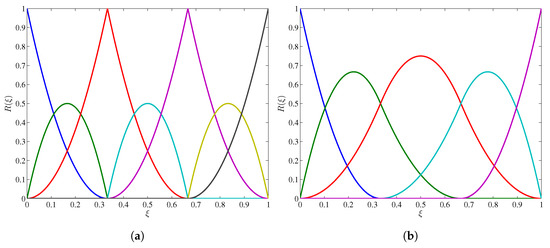
Figure 1.
(a) continuity quadratic NURBS basis functions from knot vector ; and (b) continuity quadratic NURBS basis functions from knot vector
Perfect interfaces result in continuous displacement and traction fields along the interface, i.e.,
where indicates the jump. Such conditions of weakly-discontinuity displacement can be implemented with suitable enrichment functions as in XFEM [63,64]. Moreover, in strain gradient elasticity problems, additional continuity conditions associated with higher-order terms such as displacement normal derivative and double traction [65,66]
should be satisfied along the interface. Furthermore, the interfaces in microstructure problems are often considered to be imperfect (displacement and/or traction fields are not continuous along the interface) [67,68]. However, these imperfect interface models are limited to local elasticity and do not consider strain gradients. Although the interface element was applied for mechanical problems, the same concept can be inherited and applied for multi-field problems such as piezoelectric and flexoelectric composites.
It is worth discussing the imposition of the boundary conditions in IGA approach. While the Dirichlet boundary condition can be imposed by means of least-square method [69] due to the lack of Kronecker-delta property of NURBS basis functions, the displacement gradients conditions can be applied by imposing constraint on displacement degrees of freedom with Lagrange multipliers. This idea is often used in solving strain-gradient elasticity [70] but has not been discussed in flexoelectricity modeling works. Numerical implementation of the displacement gradients conditions is shown in the next section.
In the reduced formulations without consider electric field or polarization gradient, the electric potential gradient or surface polarization needs not to be imposed. However, for modeling flexoelectric transducers, it is necessary to model the electrode on the surface of the structure by imposing the equipotential condition. This can be done by utilizing the Lagrange multiplier, as we show in the next section. Note that the equipotential has not been used in previous works on flexoelectricity using IGA. It should be remarked that recently Codony et al. [46] proposed the immersed boundary method on hierarchical B-spline for flexoelectricity problems with higher efficiency in terms of complex domain shapes smf boundary conditions handling. Moreover, the non-local conditions on non-smooth boundary (which we have neglected) was also treated.
In Table 3, we present a comparison of different numerical methods on some special features in flexoelectricity modeling, including continuity handling, computational cost (via degrees of freedom per element), the ability to enforce higher-order Dirichlet boundary conditions and material discontinuity approximation. Each numerical method comes with pros and cons and should be considered based on the desired application. For instance, mixed FE is more suitable for a simplified 2D flexoelectric problems, whereas flexoelectric domains consisting of voids or inclusions can be modeled with meshless methods.
Table 3.
Comparison of different numerical methods. and indicate quadratic elements in 2D and 3D, respectively.
3.4. Implementations
In this section, we present the computation procedure of IGA and mixed FE approaches to solve problems governed by flexoelectricity, which can serve as a numerical tool for simulating the nano-energy harvesters, sensors or actuators. For the reasons mentioned above, we consider the simplified E-formulation in Table 2, which was also the choice of the authors of [38,40], hence reasonably suitable for comparison and validation.
Mixed FEM
The requirement of continuous basis functions due to the fourth-order PDEs of flexoelectricity excludes (or at least complicates) the use of classical Lagrange polynomials. too ensure continuity displacement gradients, are introduced in the formulation and the kinematic constraint, , is imposed using Lagrange multipliers. The weak form of mechanical and electrostatic equilibrium is obtained by finding the , , , , and similarly , , and , such that,
where = and is the third-order tensor related to relaxed displacement gradient as = . The constraint is imposed in a weighted residual manner by including in Equation (33).
A nine-noded isoparametric element was proposed by Nanthakumar et al. [56]. The degrees of freedoms are and at all nodes, relaxed displacement gradients , , and at the four corner nodes and electric potential at the four corner nodes. In addition to these DOFs, the element has four Lagrange multipliers , , and at the four corner nodes. The flexoelectric element is shown in Figure 2. The biquadratic shape functions, , are used to interpolate the displacement DOFs and . Bilinear shape functions, , are used to interpolate the relaxed displacement gradients, Lagrange multipliers and electric potential, . The finite element approximation is as shown below,
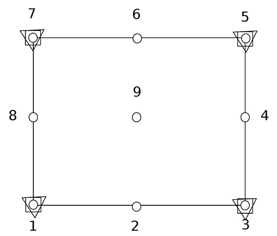
Figure 2.
A nine-noded flexoelectric element. DOFs at circles are and ; at squares are , , , and ; and at triangles are , , , and .
3.5. IGA Approach
Within the Galerkin method, both the trial and test functions are approximated by NURBS basis functions
in which and are the matrices containing the local NURBS basis functions of element e defined as
where is the NURBS basis function at control point ith and n is the number of control points of an element. In the above equation, , , and are the nodal control variables associated with displacement and electric potential of the trial and test functions, respectively, which can be written in matrix form as
The approximation of strain field , electric field , strain gradient and electric field gradient can be obtained by using differential operators ,, and on Equation (39) such that
in which , , and contain the first- and second-order partial derivative of the NURBS basis functions, respectively, defined as
Note that matrices and contain second-order derivative with respect to the physical coordinate of the basis functions. The details are presented in Appendix A. Now, based on the discretized finite elements, the weak form in Equation (30) can be re-expressed as
Finally, by substituting Equations (39) and (45) into Equation (48) and utilizing the arbitrariness of the test functions, a system of linear equations can be obtained as
where the stiffness matrices and force vectors are computed as
Note that the flexoelectric tensor for cubic symmetry crystal is given as
The symmetry of the flexoelectric tensor can be found in [71,72]. For cubic crystal, the non-zero components of flexoelectric tensor are , and while other coefficients with cycling indices are equal (e.g., ) and with odd number of indices are zeros (e.g., ) [73]. In matrix notation, the coefficients , and are denoted as , and , respectively [38].
4. Numerical Examples
4.1. Hollow Cylinder
In this first numerical example, we consider an infinitely long hollow cylinder subject to mechanical displacement and electric potential at the inner and outer surface, as depicted schematically in Figure 3a. Taking advantage of the axisymmetry, a quarter of the hollow cylinder is modeled as shown in Figure 3b, in which symmetry boundary conditions are enforced at and . This problem is an oft-used benchmark in gradient elasticity [74,75], and has been extended to flexoelectricity [39,40]. In our work, we adapt both internal energy U from [39] and electric Gibbs energy G from [40] as follows
and
where and are the two Lamé parameters, l is the length scale, and are two non-zero flexoelectric coefficients, and and are two flexoelectric coupling coefficients that related to the flexoelectric coefficients by the susceptibility such that , , and are the reciprocal susceptibility and dielectric permittivity, also related to one another by the susceptibility. These material parameters can be found in Table 4. Furthermore, due to the geometry and boundary condition, the displacement as well as the electric potential depend only on the radial r of the hollow cylinder such as
where , and are the modified Bessel functions of the first and second kind, respectively. The coefficients are determined from the boundary conditions
For numerical modeling, both formulations in Table 2 are solved with IGA, henceforth denoted as and for the formulation obtained from electric enthalpy and Gibbs energy, respectively. In addition, we also demonstrate results from second formulation with mixed FEM.
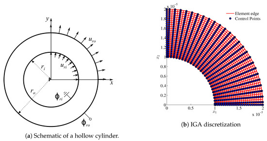
Figure 3.
Schematic of an infinitely long hollow cylinder, where the inner and outer radii are and , respectively. The inner surface is imposed by radial displacement and grounded, i.e., , whereas the radial displacement and electric potential are applied on the outer surface. Symmetry boundary conditions are enforced, such that and .
Table 4.
Material parameter for the problem depicted in Figure 3a.
For the IGA approach, we employ second-order NURBS basis functions that have continuity to model a quarter of the hollow cylinder, as shown in Figure 3b, and impose additional symmetric boundary condition on the left and bottom edges. While the homogeneous and inhomogeneous Dirichlet boundary conditions are trivial to impose [69], the boundary conditions for the displacement gradients require constraining the degrees of freedom associated with the boundary control points and their neighbors. For instance, the symmetry boundary conditions on the bottom edge in Figure 3b read
where Equation (56c) is automatically fulfilled as a result of Equation (56a). To impose Equation (56b), the nodal parameters (associated with the displacement in direction ) of the two bottom layer of control points are identical, i.e., . This can be implemented by utilizing Lagrange multipliers. On the other hand, the displacement gradient boundary conditions can be imposed effortlessly for the mixed FEM with the nodal displacement gradient.
Figure 4 presents numerical results of displacement and electric potential obtained from three approaches, showing good agreement between them. For a closer look, numerical results of radial displacement , electric potential , radial strain and circumferential strain along the radial direction with angle are presented and compared with the analytical solutions in Figure 5. Excellent agreement between the numerical and analytical results can be seen.
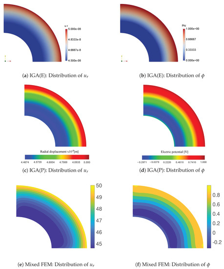
Figure 4.
Distribution of radial displacement and electric potential.
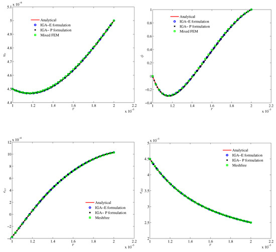
Figure 5.
Comparison of the exact and numerical results for radial displacement , electric potential , radial strain and circumferential strain as functions of radius r.
4.2. Cantilever Beam
In this example, we consider a 2D cantilever beam subjected to a point load on the right-end and having two different electrode configurations, which serve as a demonstration for a nanogenerator [38]. As depicted in Figure 6, the beam is constrained at the left-end, whereas two different electrode configuration are set up for two electrical boundary conditions. In Type-1 boundary condition, the electrode at the right-end of the beam is grounded, i.e., the electrical potential is prescribed as zero. In Type-2 condition, an electric potential difference is applied between the top and bottom electrode, e.g., the electric potential on the top is fixed to zero, whereas the bottom is induced to have an unknown equipotential V, which is solved by utilizing Lagrange multiplier. The material parameter in this study is single barium titanate (BaTi) crystal adopted from [38] and presented in Table 5. The mechanical deformation can be transform into electrical energy via the electromechanical coupling effect in the nanogenerator. The performance of this energy conversion can be evaluated by the electromechanical coupling factor given as the ratio between the electrostatic energy and the elastic energy
Consequently, the normalized piezoelectric constant is defined as
where is obtained as without considering the flexoelectric effect. Physically, the normalized piezoelectric constant indicates the enhancement of flexoelectric effect on the energy conversion. Figure 7 demonstrates the normalized piezoelectric constant as the normalized thickness varies under Type-1 configuration. The numerical results in the simplified case, where only and are non-zeros to mimic the 1D problem, are compared to the analytical solution where and excellent agreement is shown, which illustrates the great enhancement of flexoelectricity with the decrease in beam thickness. In addition, this enhancement can also be seen in the full 2D model, which is also in good agreement with the work of Abdollahi et al. [38].
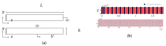
Figure 6.
(a) Schematic of a hollow cylinder. Two different types of electrical boundary condition are imposed. The upper figure describes Type-1 boundary where zero electric potential is imposed on the right edge. Type-2 boundary is demonstrated in the lower figure where zero electric potential is applied on the top edge and an unknown equipotential (due to the electrode) on the bottom edge. (b) IGA discretization (top) and mixed FEM discretization (bottom).
Table 5.
Material parameters for the problem depicted in Figure 6.
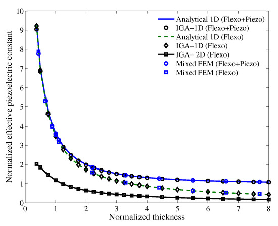
Figure 7.
Effective normalized piezoelectric constant obtained with Type-1 boundary condition.
We further investigate the difference in the normalized effective piezoelectric constant with two different electrical boundary conditions and present the numerical results in Figure 8. In both boundary condition setups, as the beam thickness decreases, the normalized effective piezoelectric constant increases, which is expected due to the size effect nature of flexoelectricity. Notably, Type-1 boundary condition seems to be more effective than Type-2. Furthermore, both IGA and mixed FEM approach give the same prediction on the performance of two boundary condition types. For a closer look, we present the electric potential distribution for two electrical boundary conditions computed from IGA and mixed FEM in Figure 9 with the height and length of the beam being and , respectively. The results from the two methods are in agreement. For Type-1 boundary condition, the electric potential difference is highest at the left end of the beam, where strain gradient is largest. As for the Type-2 boundary condition, the induced electric potential at the top electrode is around .
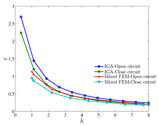
Figure 8.
Effective piezoelectric constant under different electrical boundary conditions.
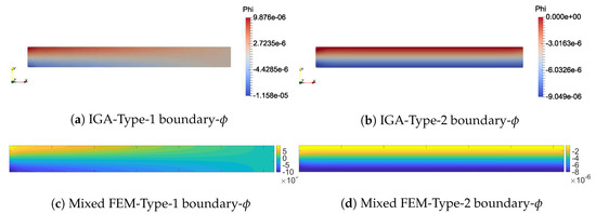
Figure 9.
Electric potential distribution under Type-1 and Type-2 electrical boundary conditions.
Additionally, we also carried out a three-dimensional simulation of a cantilever beam under Type-2 electrical boundary condition by using IGA. The 3D beam is assumed to have square cross-section, where the width is equal to the height h. The length of the beam as well as the applied force on the right surface are unchanged as in the two-dimensional case. Figure 10 shows the induced electric potential. A similar response has been observed as in 2D case, where largest electric potential is at the left end. Nevertheless, the electric potential at the top electrode has the value of .
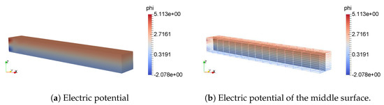
Figure 10.
Electric potential of a 3D bending flexoelectric beam.
We also study the converse flexoelectric effect from the electrical boundary condition. While the mechanical point load is omitted, a uniform electric field with magnitude is applied by setting the electric potential to be on the bottom electrode. In this case, the beam behaves as an actuator and induces bending curvature, which is shown in Figure 11b. The calculated curvature of the bending beam due to converse flexoelectric effect is in good agreement with both numerical results from [38] and the experimental ones from Bursian and OI [76]. Further investigation on the distribution of electric field in the thickness direction of the beam is shown in Figure 11a, which is also in agreement with the result from [38]. Non-uniform distribution of electric field can be observed, especially at the region near the top and bottom edge of the beam, which yields high electric field gradient and consequently induces deformation. Note that the considered flexoelectric beams do not account for the resistive load [10] or the rectifying circuit [77,78]. In [77], a piezoelectric structure is analyzed along with its circuit connections. In addition, in [78], comparisons between the charge type Hamiltonian and voltage type Hamiltonian are performed to identify the output power and voltage of the piezoelectric energy harvester. Development of a fully combined flexoelectric generator and interface circuit might be of significance in the future.
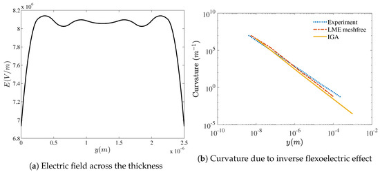
Figure 11.
Beam under electrical load.
4.3. Truncated Pyramid
This section presents the numerical results of a two-dimensional truncated pyramid under compression with different type of boundary conditions, as adopted from [38]. Figure 12 depicts the schematic of a truncated pyramid whose top surface is grounded with zero electric potential, whereas the bottom surface is attached with an electrode that results in the equipotential condition on it. Two mechanical boundary conditions are considered, namely the rigid boundary condition where the bottom surface is constrained in direction and the top surface is subjected to uniform load F, and the flexible boundary condition where both the bottom and top surfaces are subjected to uniform compression load F. For numerical modeling, the problem is discretized by quadratic -continuity NURBS basis functions, as shown in Figure 12b as well as by mixed FEM as in Figure 12c.
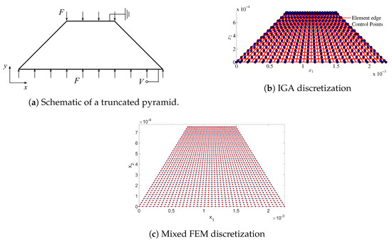
Figure 12.
Schematic and IGA discretization of a truncated pyramid.
Numerical results of electric potential and compression strain for the rigid boundary condition from IGA and Mixed FEM are presented in Figure 13 and for flexible boundary condition from IGA are shown in Figure 14. Good agreement can be observed between the two methods as well as with the reference results [38]. In rigid model, our IGA and mixed FEM approaches predict the equipotential of bottom electrode to be and mV, respectively, while the reference result is mV [38]. Similarly, in flexible model, the bottom equipotential is mV, agreeing with the value of mV from [38].
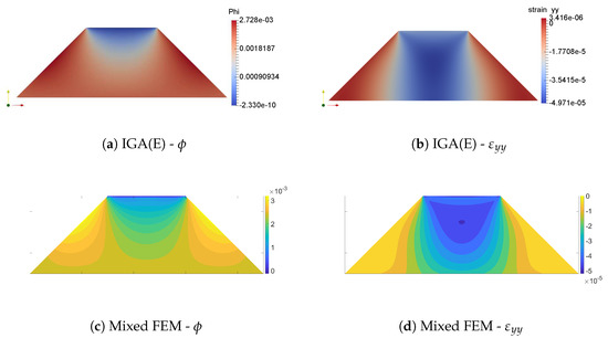
Figure 13.
Rigid boundary condition.
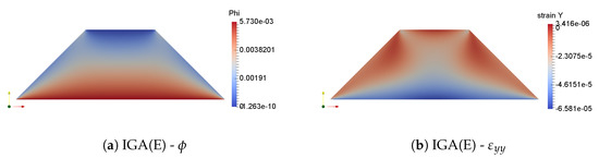
Figure 14.
Flexible boundary condition.
Additionally, a three-dimensional version of the truncated pyramid is also studied. The geometric parameters are kept as in 2D case, so that the top and bottom surfaces now have dimension of and , respectively. The flexible boundary condition is considered, where the applied force F is identical from the 2D case. The numerical result from IGA is shown in Figure 15. As can be seen in Figure 15c, the electric potential in 3D model is very similar to that of 2D model. However, the induced potential on the top electrode is now , three orders of magnitude greater than the result predicted from 2D model.
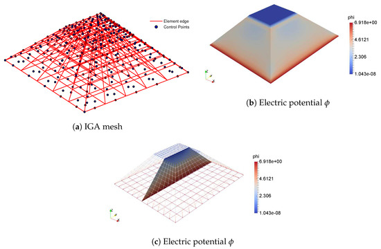
Figure 15.
3D pyramid.
5. Discussion
Since its discovery, flexoelectricity bears significance because of its potential to aid developing novel electromechanical coupling devices. To fully utilize this effect, both experimental and simulation approaches are necessary. In view of simulation, in this paper, we provide a generalized formulation of flexoelectricity as the extension from gradient elasticity. Remarkably, the boundary value problems that involve fourth-order PDE in flexoelectricity, necessitating continuity, are obtained from electric enthalpy as well as electric Gibbs free energy. To overcome the high-order continuity, we employ isogeometric analysis and mixed finite element, where detailed implementations are reported. We solved benchmark problems using these methods on 2D and 3D flexoelectric problems. The source codes are provided and can be used to study more complex problems.
Author Contributions
Conceptualization, X.Z., B.H.N., S.S.N., T.Q.T., N.A., and T.R.; methodology, X.Z., B.H.N., S.S.N., T.Q.T., N.A., and T.R.; software, B.H.N., S.S.N., and T.Q.T.; validation, B.H.N., S.S.N., and T.Q.T.; formal analysis, B.H.N., S.S.N., and T.Q.T.; investigation, B.H.N., S.S.N., and T.Q.T.; writing, X.Z., B.H.N., S.S.N., T.Q.T., N.A., and T.R.; visualization, B.H.N., S.S.N., and T.Q.T.; and supervision, X.Z. and T.R. All authors have read and agreed to the published version of the manuscript.
Funding
This research received no external funding.
Acknowledgments
The authors extend their appreciation to the Distinguished Scientist Fellowship Program (DSFP) at King Saud University for funding this work.
Conflicts of Interest
The authors declare no conflict of interest.
Appendix A. Second-Order Derivative of NURBS Basis Functions
The computation of second-order derivative with respect to the physical coordinate of the basis functions can be achieved by first noticing that the first-order derivative of the basis functions with respect to the parametric coordinate is computed from the Jacobian matrix
Next, by taking the second-order derivative with respect to the parametric coordinate and re-arranging, the second-order derivative with respect to the physical coordinate is determined from
References
- Tolpygo, K. Long wavelength oscillations of diamond-type crystals including long range forces. Sov. Phys.-Solid State 1963, 4, 1297–1305. [Google Scholar]
- Kogan, S.M. Piezoelectric effect during inhomogeneous deformation and acoustic scattering of carriers in crystals. Sov. Phys.-Solid State 1964, 5, 2069–2070. [Google Scholar]
- Huang, W.; Yan, X.; Kwon, S.R.; Zhang, S.; Yuan, F.G.; Jiang, X. Flexoelectric strain gradient detection using Ba0. 64Sr0. 36TiO3 for sensing. Appl. Phys. Lett. 2012, 101, 252903. [Google Scholar] [CrossRef]
- Kwon, S.R.; Huang, W.; Zhang, S.; Yuan, F.G.; Jiang, X. Study on a flexoelectric microphone using barium strontium titanate. J. Micromech. Microeng. 2016, 26, 045001. [Google Scholar] [CrossRef]
- Merupo, V.I.; Guiffard, B.; Seveno, R.; Tabellout, M.; Kassiba, A. Flexoelectric response in soft polyurethane films and their use for large curvature sensing. J. Appl. Phys. 2017, 122, 144101. [Google Scholar] [CrossRef]
- Bhaskar, U.K.; Banerjee, N.; Abdollahi, A.; Wang, Z.; Schlom, D.G.; Rijnders, G.; Catalan, G. A flexoelectric microelectromechanical system on silicon. Nat. Nanotechnol. 2016, 11, 263. [Google Scholar] [CrossRef]
- Zhang, S.; Liu, K.; Xu, M.; Shen, S. A curved resonant flexoelectric actuator. Appl. Phys. Lett. 2017, 111, 082904. [Google Scholar] [CrossRef]
- Rey, A.D.; Servio, P.; Herrera-Valencia, E. Bioinspired model of mechanical energy harvesting based on flexoelectric membranes. Phys. Rev. E 2013, 87, 022505. [Google Scholar] [CrossRef]
- Jiang, X.; Huang, W.; Zhang, S. Flexoelectric nano-generator: Materials, structures and devices. Nano Energy 2013, 2, 1079–1092. [Google Scholar] [CrossRef]
- Deng, Q.; Kammoun, M.; Erturk, A.; Sharma, P. Nanoscale flexoelectric energy harvesting. Int. J. Solids Struct. 2014, 51, 3218–3225. [Google Scholar] [CrossRef]
- Choi, S.B.; Kim, G.W. Measurement of flexoelectric response in polyvinylidene fluoride films for piezoelectric vibration energy harvesters. J. Phys. D Appl. Phys. 2017, 50, 075502. [Google Scholar] [CrossRef]
- Liang, X.; Hu, S.; Shen, S. Nanoscale mechanical energy harvesting using piezoelectricity and flexoelectricity. Smart Mater. Struct. 2017, 26, 035050. [Google Scholar] [CrossRef]
- Zhu, R.; Wang, Z.; Ma, H.; Yuan, G.; Wang, F.; Cheng, Z.; Kimura, H. Poling-free energy harvesters based on robust self-poled ferroelectric fibers. Nano Energy 2018, 50, 97–105. [Google Scholar] [CrossRef]
- Lu, H.; Bark, C.W.; De Los Ojos, D.E.; Alcala, J.; Eom, C.B.; Catalan, G.; Gruverman, A. Mechanical writing of ferroelectric polarization. Science 2012, 336, 59–61. [Google Scholar] [CrossRef] [PubMed]
- Lu, H.; Liu, S.; Ye, Z.; Yasui, S.; Funakubo, H.; Rappe, A.M.; Gruverman, A. Asymmetry in mechanical polarization switching. Appl. Phys. Lett. 2017, 110, 222903. [Google Scholar] [CrossRef]
- Guo, R.; Shen, L.; Wang, H.; Lim, Z.; Lu, W.; Yang, P.; Gruverman, A.; Venkatesan, T.; Feng, Y.P.; Chen, J. Tailoring Self-Polarization of BaTiO3 Thin Films by Interface Engineering and Flexoelectric Effect. Adv. Mater. Interfaces 2016, 3, 1600737. [Google Scholar] [CrossRef]
- Yang, M.M.; Kim, D.J.; Alexe, M. Flexo-photovoltaic effect. Science 2018, 360, 904–907. [Google Scholar] [CrossRef]
- Liu, Y.; Chen, J.; Deng, H.; Hu, G.; Zhu, D.; Dai, N. Anomalous thermoelectricity in strained Bi 2 Te 3 films. Sci. Rep. 2016, 6, 32661. [Google Scholar] [CrossRef]
- Nguyen, T.D.; Mao, S.; Yeh, Y.W.; Purohit, P.K.; McAlpine, M.C. Nanoscale flexoelectricity. Adv. Mater. 2013, 25, 946–974. [Google Scholar] [CrossRef]
- Zubko, P.; Catalan, G.; Tagantsev, A.K. Flexoelectric effect in solids. Annu. Rev. Mater. Res. 2013, 43. [Google Scholar] [CrossRef]
- Yudin, P.; Tagantsev, A. Fundamentals of flexoelectricity in solids. Nanotechnology 2013, 24, 432001. [Google Scholar] [CrossRef] [PubMed]
- Krichen, S.; Sharma, P. Flexoelectricity: A perspective on an unusual electromechanical coupling. J. Appl. Mech. 2016, 83, 030801. [Google Scholar] [CrossRef]
- Maranganti, R.; Sharma, N.; Sharma, P. Electromechanical coupling in nonpiezoelectric materials due to nanoscale nonlocal size effects: Green’s function solutions and embedded inclusions. Phys. Rev. B 2006, 74, 014110. [Google Scholar] [CrossRef]
- Mindlin, R.D. Polarization gradient in elastic dielectrics. Int. J. Solids Struct. 1968, 4, 637–642. [Google Scholar] [CrossRef]
- Sahin, E.; Dost, S. A strain-gradients theory of elastic dielectrics with spatial dispersion. Int. J. Eng. Sci. 1988, 26, 1231–1245. [Google Scholar] [CrossRef]
- Majdoub, M.; Sharma, P.; Çağin, T. Dramatic enhancement in energy harvesting for a narrow range of dimensions in piezoelectric nanostructures. Phys. Rev. B 2008, 78, 121407. [Google Scholar] [CrossRef]
- Majdoub, M.; Sharma, P.; Çağin, T. Erratum: Dramatic enhancement in energy harvesting for a narrow range of dimensions in piezoelectric nanostructures [Phys. Rev. B 78, 121407 (R)(2008)]. Phys. Rev. B 2009, 79, 159901. [Google Scholar] [CrossRef]
- Majdoub, M.; Sharma, P.; Cagin, T. Enhanced size-dependent piezoelectricity and elasticity in nanostructures due to the flexoelectric effect. Phys. Rev. B 2008, 77, 125424. [Google Scholar] [CrossRef]
- Majdoub, M.S.; Sharma, P.; Çağin, T. Erratum: Enhanced size-dependent piezoelectricity and elasticity in nanostructures due to the flexoelectric effect [Phys. Rev. B77, 125424 (2008)]. Phys. Rev. B 2009, 79. [Google Scholar] [CrossRef]
- Sharma, N.; Landis, C.; Sharma, P. Piezoelectric thin-film superlattices without using piezoelectric materials. J. Appl. Phys. 2010, 108, 024304. [Google Scholar] [CrossRef]
- Hu, S.; Shen, S. Variational principles and governing equations in nano-dielectrics with the flexoelectric effect. Sci. China Physics, Mech. Astron. 2010, 53, 1497–1504. [Google Scholar] [CrossRef]
- Kuang, Z.B. Some problems in electrostrictive and magnetostrictive materials. Acta Mech. Solida Sin. 2007, 20, 219–227. [Google Scholar] [CrossRef]
- Kuang, Z. Some variational principles in electroelastic media under finite deformation. Sci. China Ser. Physics, Mech. Astron. 2008, 51, 1390–1402. [Google Scholar] [CrossRef]
- Kuang, Z.b. Internal energy variational principles and governing equations in electroelastic analysis. Int. J. Solids Struct. 2009, 46, 902–911. [Google Scholar] [CrossRef][Green Version]
- Kuang, Z.B. Theory Electroelasticity; Springer: Berlin/Heidelberg, Germany, 2014. [Google Scholar]
- Liu, L. On energy formulations of electrostatics for continuum media. J. Mech. Phys. Solids 2013, 61, 968–990. [Google Scholar] [CrossRef]
- Liu, L. An energy formulation of continuum magneto-electro-elasticity with applications. J. Mech. Phys. Solids 2014, 63, 451–480. [Google Scholar] [CrossRef]
- Abdollahi, A.; Peco, C.; Millan, D.; Arroyo, M.; Arias, I. Computational evaluation of the flexoelectric effect in dielectric solids. J. Appl. Phys. 2014, 116, 093502. [Google Scholar] [CrossRef]
- Mao, S.; Purohit, P.K.; Aravas, N. Mixed finite-element formulations in piezoelectricity and flexoelectricity. Proc. R. Soc. A 2016, 472, 20150879. [Google Scholar] [CrossRef]
- Deng, F.; Deng, Q.; Yu, W.; Shen, S. Mixed Finite Elements for Flexoelectric Solids. J. Appl. Mech. 2017, 84, 081004. [Google Scholar] [CrossRef]
- Ghasemi, H.; Park, H.S.; Rabczuk, T. A level-set based IGA formulation for topology optimization of flexoelectric materials. Comput. Methods Appl. Mech. Eng. 2017, 313, 239–258. [Google Scholar] [CrossRef]
- Thai, T.Q.; Rabczuk, T.; Zhuang, X. A large deformation isogeometric approach for flexoelectricity and soft materials. Comput. Methods Appl. Mech. Eng. 2018, 341, 718–739. [Google Scholar] [CrossRef]
- Nguyen, B.; Zhuang, X.; Rabczuk, T. Numerical model for the characterization of Maxwell-Wagner relaxation in piezoelectric and flexoelectric composite material. Comput. Struct. 2018, 208, 75–91. [Google Scholar] [CrossRef]
- Nguyen, B.; Zhuang, X.; Rabczuk, T. NURBS-based formulation for nonlinear electro-gradient elasticity in semiconductors. Comput. Methods Appl. Mech. Eng. 2019, 346, 1074–1095. [Google Scholar] [CrossRef]
- Yvonnet, J.; Liu, L. A numerical framework for modeling flexoelectricity and Maxwell stress in soft dielectrics at finite strains. Comput. Methods Appl. Mech. Eng. 2017, 313, 450–482. [Google Scholar] [CrossRef]
- Codony, D.; Marco, O.; Fernández-Méndez, S.; Arias, I. An Immersed Boundary Hierarchical B-spline method for flexoelectricity. arXiv 2019, arXiv:1902.02567. [Google Scholar] [CrossRef]
- Roy, P.; Roy, D. Peridynamics model for flexoelectricity and damage. Appl. Math. Model. 2019, 68, 82–112. [Google Scholar] [CrossRef]
- Toupin, R.A. The elastic dielectric. J. Ration. Mech. Anal. 1956, 5, 849–915. [Google Scholar] [CrossRef]
- Mindlin, R.D.; Eshel, N. On first strain-gradient theories in linear elasticity. Int. J. Solids Struct. 1968, 4, 109–124. [Google Scholar] [CrossRef]
- Abdollahi, A.; Millán, D.; Peco, C.; Arroyo, M.; Arias, I. Revisiting pyramid compression to quantify flexoelectricity: A three-dimensional simulation study. Phys. Rev. B 2015, 91, 104103. [Google Scholar] [CrossRef]
- Abdollahi, A.; Domingo, N.; Arias, I.; Catalan, G. Converse flexoelectricity yields large piezoresponse force microscopy signals in non-piezoelectric materials. Nat. Commun. 2019, 10, 1266. [Google Scholar] [CrossRef]
- He, B.; Javvaji, B.; Zhuang, X. Characterizing Flexoelectricity in Composite Material Using the Element-Free Galerkin Method. Energies 2019, 12, 271. [Google Scholar] [CrossRef]
- Liu, G.R. Meshfree Methods: Moving Beyond the Finite Element Method; CRC Press: Boca Raton, FL, USA, 2009. [Google Scholar]
- Cordes, L.; Moran, B. Treatment of material discontinuity in the element-free Galerkin method. Comput. Methods Appl. Mech. Eng. 1996, 139, 75–89. [Google Scholar] [CrossRef]
- Krongauz, Y.; Belytschko, T. EFG approximation with discontinuous derivatives. Int. J. Numer. Methods Eng. 1998, 41, 1215–1233. [Google Scholar] [CrossRef]
- Nanthakumar, S.; Zhuang, X.; Park, H.S.; Rabczuk, T. Topology optimization of flexoelectric structures. J. Mech. Phys. Solids 2017, 105, 217–234. [Google Scholar] [CrossRef]
- Deng, F.; Deng, Q.; Shen, S. A three-dimensional mixed finite element for flexoelectricity. J. Appl. Mech. 2018, 85, 031009. [Google Scholar] [CrossRef]
- Les Piegl, W.T. The NURBS Book; Springer: Berlin/Heidelberg, Germany, 1997. [Google Scholar]
- Cottrell, J.; Hughes, T.; Bazilevs, Y. Isogeometric Analysis: Toward Integration of CAD and FEA; John Wiley & Sons Inc.: Hoboken, NJ, USA, 2009. [Google Scholar]
- Camacho, G.T.; Ortiz, M. Computational modelling of impact damage in brittle materials. Int. J. Solids Struct. 1996, 33, 2899–2938. [Google Scholar] [CrossRef]
- Schrefler, B.A.; Secchi, S.; Simoni, L. On adaptive refinement techniques in multi-field problems including cohesive fracture. Comput. Methods Appl. Mech. Eng. 2006, 195, 444–461. [Google Scholar] [CrossRef]
- de Borst, R. Fluid flow in fractured and fracturing porous media: A unified view. Mech. Res. Commun. 2017, 80, 47–57. [Google Scholar] [CrossRef]
- Sukumar, N.; Chopp, D.L.; Moës, N.; Belytschko, T. Modeling holes and inclusions by level sets in the extended finite-element method. Comput. Methods Appl. Mech. Eng. 2001, 190, 6183–6200. [Google Scholar] [CrossRef]
- Sukumar, N.; Huang, Z.; Prévost, J.H.; Suo, Z. Partition of unity enrichment for bimaterial interface cracks. Int. J. Numer. Methods Eng. 2004, 59, 1075–1102. [Google Scholar] [CrossRef]
- Shu, J.Y.; King, W.E.; Fleck, N.A. Finite elements for materials with strain gradient effects. Int. J. Numer. Methods Eng. 1999, 44, 373–391. [Google Scholar] [CrossRef]
- Soh, A.K.; Wanji, C. Finite element formulations of strain gradient theory for microstructures and the C0–1 patch test. Int. J. Numer. Methods Eng. 2004, 61, 433–454. [Google Scholar] [CrossRef]
- Gu, S.; He, Q.C. Interfacial discontinuity relations for coupled multifield phenomena and their application to the modeling of thin interphases as imperfect interfaces. J. Mech. Phys. Solids 2011, 59, 1413–1426. [Google Scholar] [CrossRef]
- Liu, J.T.; He, B.; Gu, S.T.; He, Q.C. Implementation of a physics-based general elastic imperfect interface model in the XFEM and LSM context. Int. J. Numer. Methods Eng. 2018, 115, 1499–1525. [Google Scholar] [CrossRef]
- Nguyen, V.P.; Anitescu, C.; Bordas, S.P.; Rabczuk, T. Isogeometric analysis: An overview and computer implementation aspects. Math. Comput. Simul. 2015, 117, 89–116. [Google Scholar] [CrossRef]
- Fischer, P.; Klassen, M.; Mergheim, J.; Steinmann, P.; Müller, R. Isogeometric analysis of 2D gradient elasticity. Comput. Mech. 2011, 47, 325–334. [Google Scholar] [CrossRef]
- Shu, L.; Wei, X.; Pang, T.; Yao, X.; Wang, C. Symmetry of flexoelectric coefficients in crystalline medium. J. Appl. Phys. 2011, 110, 104106. [Google Scholar] [CrossRef]
- Le Quang, H.; He, Q.C. The number and types of all possible rotational symmetries for flexoelectric tensors. Proc. R. Soc. Lond. A Math. Phys. Eng. Sci. 2011, 467, 2369–2386. [Google Scholar] [CrossRef]
- Hong, J.; Vanderbilt, D. First-principles theory and calculation of flexoelectricity. Phys. Rev. B 2013, 88, 174107. [Google Scholar] [CrossRef]
- Gao, X.L.; Park, S. Variational formulation of a simplified strain gradient elasticity theory and its application to a pressurized thick-walled cylinder problem. Int. J. Solids Struct. 2007, 44, 7486–7499. [Google Scholar] [CrossRef]
- Aravas, N. Plane-strain problems for a class of gradient elasticity models—A stress function approach. J. Elast. 2011, 104, 45–70. [Google Scholar] [CrossRef]
- Bursian, E.; OI, Z. Changes in curvature of a ferroelectric film due to polarization. Sov. Phys. Solid State, USSR 1968, 10, 1121–1124. [Google Scholar]
- Lumentut, M.; Shu, Y. A unified electromechanical finite element dynamic analysis of multiple segmented smart plate energy harvesters: Circuit connection patterns. Acta Mech. 2018, 229, 4575–4604. [Google Scholar] [CrossRef]
- Lumentut, M.; Howard, I. Intrinsic electromechanical dynamic equations for piezoelectric power harvesters. Acta Mech. 2017, 228, 631–650. [Google Scholar] [CrossRef]
Sample Availability: Detailed data and codes are available from the authors by request. |
© 2020 by the authors. Licensee MDPI, Basel, Switzerland. This article is an open access article distributed under the terms and conditions of the Creative Commons Attribution (CC BY) license (http://creativecommons.org/licenses/by/4.0/).