New Adaptive High Starting Torque Scalar Control Scheme for Induction Motors Based on Passivity

Abstract

A novel adaptive high starting torque (HST) scalar control scheme (SCS) for induction motors (IM) is proposed in this paper. It uses a new adaptive-passivity-based controller (APBC) proposed herein for a class of nonlinear systems, with linear explicit parametric dependence and linear stable internal dynamics, which encompasses the IM dynamical model. The main advantage of the HST-SCS includes the ability to move loads with starting-torque over the nominal torque with a simple and cost-effective implementation without needing a rotor speed sensor, variable observers, or parameter estimators. The proposed APBC is based on a direct control scheme using a normalized fixed gain (FG) to fine-tune the adaptive controller parameters. The basic SCS for induction motors (IM) and the HST-SCS were applied to an IM of 200 HP and tested using a real-time simulator controller OPAL-RT showing the achievement of the proposal goal.

1. Introduction

Compared to direct current electric motors, induction motors (IMs) have a lower cost and higher efficiency, require lower maintenance, and have been replacing them in variable speed operations with increasing use in the past twenty years [1]. In variable speed applications, the IM is fed by different types of alternating current (AC) drives [2], which differ in their performance with respect to the starting torque, transient speed behavior, and steady-state speed-accuracy of the desired speed [1]. For low, medium, and high-performance applications, three main control schemes are used: scalar control scheme (SCS) [3], direct torque control (DTC) [4], and field-oriented control (FOC) [5,6] respectively. There is also a simpler AC/AC soft starter based on thyristors [3], but it does not allow variable speed operation. It only reduces the starting stator current while moving low starting torque loads. This reduction is made by reducing the starting voltage applied to the motor.

The AC drive with a rotor speed closed loop (CL), based on FOC or DTC, is used for high-performance applications, such as winding and takeoffs. Its capabilities consist of starting with torque around 150% of the nominal torque, having a rapid and no oscillatory transient speed behavior, and exhibiting 0.01% of steady-state speed accuracy. It needs parameter estimators to compute its characteristic variable slip frequency of operation. The AC drive based on sensorless DTC or sensorless FOC, is used for medium-performance applications. These consist of cranes, positive displacement pumps, and compressors. Its capabilities consist of starting with torque around 120% of the nominal torque, having a rapid and no oscillatory transient speed behavior, and 0.1% of steady-state speed accuracy. It needs parameter estimators and variable observers to compute its characteristic direct torque and flux control. In contrast, the cheapest AC-drive-based SCS is used for low-performance applications. Examples of these include blowers, fans, and centrifugal pumps. SCS only needs the rated voltage per phase and the frequency taken from the motor data plate. It moves loads needing a starting torque lower than 40% of the nominal torque [7] with 1% to 3% of steady-state speed accuracy and nonrapid and even oscillatory transient behavior [8,9,10]. These facts about SCS remain even if a CL speed control is considered as mainly improving steady-state accuracy [9]. This is the reason why FOC is finally proposed in [10] to reach a higher performance. Oscillatory transient behavior issues of the SCS are studied in detail in [11].

Several research works aim to improve the simplest SCS [12,13,14,15,16,17]. Compared to the DTC [4] and the FOC [5,6], the SCS needs neither parameter estimators nor estimator or sensor of the rotor speed. SCS schemes [3,12,13,14,15,16,17] assume that the electrical angular speed is equal to the reference rotor angular speed, neglecting the slip, or equals to the reference rotor angular speed plus an estimated slip. These are the simplest and most effective ways the estimated rotor angle is implemented. Improvements in works [12,13,14,15] consider estimating the slip to improve the rotor steady-state speed-accuracy. The electromagnetic torque is estimated in [12], and later the slip is based on this estimate. The gap power is estimated in [13] and then the slip is estimated, adjusting also the boost voltage. The slip is calculated based on a stator flux observer in [14], which depends on parameter estimators. A simpler slip calculation scheme is proposed in [15], where the computing depends on the rated stator current and the rated slip. The speed control of all these SCS schemes has an open-loop (OL) speed control.

In addition, to improve the steady-state rotor speed accuracy of the SCS, a CL speed controller is proposed in [16]. The required electrical frequency is set by a CL speed fuzzy controller in [16]. It depends on the measurement of a rotor angular speed sensor. A rotor angular speed observer based on a spectral search method is proposed in [17] to improve the SCS speed monitoring. It is suggested in [17] that this monitoring could be used in other works to develop a CL sensorless SCS, but this is not fully addressed by [17].

All these schemes [12,13,14,15,16,17] aim to improve the accuracy of the steady-state rotor speed. They all need parameter estimators, depending on the accuracy of the estimates. The low starting torque issue of the SCS is not addressed in these references from [12,13,14,15,16,17]. It is in this paper where a solution is suggested.

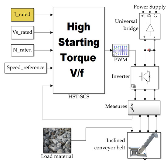
The mining and minerals industry, for instance, has machinery such as conveyor belts. These need high starting torque but no steady-state speed accuracy. One employed solution is to consider AC drives with a DTC or FOC scheme, paying an over cost. Another solution considers an AC drive with SCS to move the belt conveyors unloaded at the start. This last solution has an issue when unforeseen detentions occur. This paper aims to propose an alternative simple solution to move high starting-torque loads. It uses for current-control purposes the same current sensors used today by the basic SCS for motor protection. Compared to the DTC [4] and the FOC [5,6], the proposed high starting torque (HST)-SCS needs neither parameter estimators, variable observers, nor estimator or sensor of the rotor speed. As a result, it moves loads needing a starting torque around 100% of the nominal torque from 1% to 3% of steady-state speed accuracy and nonrapid and even oscillatory transient behavior [8,9,10]. It expands the applications of the SCS but is not capable of substituting the FOC nor DTC schemes.

The main contribution of this paper is the proposal of an HST-SCS. It adds a CL adaptive-passivity-based controller (APBC) for current to the basic SCS. This is based on the adaptive theory from [18,19] developed for linear dynamical systems but extended herein for a class of nonlinear dynamical systems expressed in the normal form, which has a linear explicit parametric dependence with a linear internal dynamic and encompasses the IM model. The use of normalized FG is proposed to adjust the adaptive controller parameters.

The paper is organized as follows: Section 2 describes the IM model, the basic SCS method, and the APBC basis. The proposed APBC method for a class of nonlinear systems is proposed in Section 3. Experimental results comparing basic SCS and the proposed HST-SCS are described in Section 4. Finally, in Section 5, some conclusions are drawn.

2. Preliminaries

The design and performance of the proposed HST-SCS for IM will be compared to the basic SCS for the IM described in this section. Both schemes make use of several concepts and theories also described in what follows.

2.1. Basic SCS for IM

The steady-state IM-equivalent circuit per phase is described in detail in Appendix A.1 [20]. The basic SCS considers a P controller to keep constant magnetization at different electrical frequencies as shown in the following equation:

$$V_s^{\ast }=\{\begin{array}{c}\begin{array}{ccc}{P}_1{\omega }_e^{\ast }+\sqrt{2}{V}_{boost},& \mathrm{with} P_1=\frac{\sqrt{2}p}{2\pi }\left(\frac{V_{s\_rated}}{f_{rated}}-\frac{V_{boost}}{fc}\right)& \mathrm{for} f_{min}<f<f_c,\end{array}\\ \begin{array}{ccc}{P}_2{\omega }_e^{\ast },& \mathrm{with} P_2=\frac{\sqrt{2}p}{2\pi }\left(\frac{V_{s\_rated}}{f_{rated}}\right)& \mathrm{for} f_c<f<f_{rated},\end{array}\end{array}$$

(1)

where $V_s^{\ast }$ is the required amplitude of the phase stator voltage to be applied in order to achieve the required electrical angular frequency ${\omega }_e^{\ast }$. In practice, ${\omega }_e^{\ast }$ is considered to be equal to the required rotor angular speed multiplied by the pair of poles ${\omega }_{\mathrm{r}}^{\ast }p$, neglecting the rotor angular slip. $V_{s\_rated}$ is the rated phase voltage from the motor data plate, p is the pair of poles, f_rated is the motor rated frequency in Hz, and the $V_{boost}$ has a value of up to 25% of $V_{s\_rated}$ in [21] and operates from the minimum frequency $f_{min}$ (with a value up to 6% of $f_{rated}$ in [21]) to the low-frequency $f_c$ (with a value up to 40% of $f_{rated}$ in [21]). The $V_{boost}$ is a controller bias or offset needed to deliver a certain amount of starting torque according to Equation (A4):

$$T_{em}=3\left(\frac{p}{2}\right){\left(\frac{V_s}{{\omega }_e}\right)}^2\frac{R_r{\omega }_{slip}}{R_r{}^2+{\left({\omega }_{slip}{L^{\prime }}_r\right)}^2}$$

(2)

The scalar control aims to keep a constant flux modulus ($\left|\phi \right|)$, neglecting the stator voltage drop in the stator impedance ($R_s{i}_s+j{\omega }_e{L}_s^{\prime }{i}_s\approx 0)$. After that, the Kirchhoff’s voltage law equation for the stator (A1) was simplified and shows the dependence between the flux modulus ($\left|\phi \right|)$, the frequency ${\omega }_e$, and the modulus of the voltage applied to the motor, according to

$$u_s=\stackrel{\approx 0}{\overbrace{\left(R_s{i}_s+j{\omega }_e{L}_s^{\prime }{i}_s\right)}}+j{\omega }_e\stackrel{\phi }{\overbrace{L_m{i}_m}}=>u_s\approx j{\omega }_e\phi =>\left|\phi \right|~\frac{\stackrel{V_s}{\overbrace{\left|u_s\right|}}}{{\omega }_e}.$$

(3)

Thus, the amplitude of the rated voltage per phase and the rated electrical angular frequency are related as $P_2=\frac{\surd 2p}{2\pi }\left(\frac{V_{s\_rated}}{frated}\right)=\left|{\phi }_{rated}\right|$, which is kept constant over $f_c$ throughout Equation (1). From this result, it can also be shown that at low speed, the required voltage $V_{\mathrm{s}}^{\ast }=P_2{\omega }_e^{\ast }$ is low, and the stator impedance is no longer neglectable. This is the reason why a $V_{boost}$ is applied under $f_c$ through the Equation (1) to assure the existence of flux and torque in this case. Finally, when operating at speeds higher than the rated speed ${\omega }_{e\_rated}$, a saturator needs to be used after the P controller. It limits the stator voltage to the safe limit $V_{s\_rated}$, thus protecting the IM.

After applying the Park transformation $e^{-j\rho }$ [22], the two-phase α–β instantaneous signals fixed at a stationary reference frame can be obtained from the d–q amplitude magnitudes rotating at the synchronous reference frame; thus, $u_{s\propto \beta }^{\ast }=e^{-j\rho }{V}_{sdq}^{\ast }$. Similarly, from the α–β instantaneous signals, the d–q amplitude magnitudes can be obtained through $I_{sdq}=e^{-j\rho }{i}_{s\propto \beta }$.

In addition, using the Clarke transformation $T_{2\to 3}$ [23] from the two-phase α–β instantaneous signals fixed at the stationary reference frame, the three-phasic instantaneous signals can be obtained through $u_s={\left[\begin{array}{ccc}{u}_a& u_b& u_c\end{array}\right]}^T=T_{2\to 3}{u}_{s\propto \beta }^{\ast }$ and vice versa $i_{s\alpha \beta }=\left[\begin{array}{cc}{i}_{s\alpha }& i_{s\beta }\end{array}\right]=T_{3\to 2}{i}_s$.

The general diagram of the basic SCS for IM that will be used in this paper for comparison purposes is shown in Figure 1, taken from [21]. It does not make use of parameter estimators when compared to DTC [4] or FOC [5,6], using only the rated voltage per phase from the motor data plate and sensors of the stator current consumption to check the proper IM functioning for its protection. The setpoint of the required rotor angular speed ${\omega }_r^{\ast }$ is established by the operator, and the SCS automatically defines the required stator voltage $V_{sd}^{\ast }$ and electrical frequency ${\omega }_e$.

The SCS scheme described in Figure 1 is simple and effective. It is used for applications needing low starting torque and a steady-state speed accuracy up to 3%. To operates motor loads needing HST, some issues are faced which are described in the next section.

2.2. Problem Statement

After applying the basic SCS for IM, the following issues are faced:

(a)

HST: To keep the constant flux given in (3), basic SCS uses the controller (1), which has a low starting torque issue. This is due to the low applied starting voltage, even after applying the $V_{boost}$, because the torque (2) is proportional to the square of the quotient between the phase rated stator voltage and rated electrical frequency. Thus, an alternative method controlling the required stator current $i_s^{\ast }$ to have HST is proposed next.

(b)

Nonlinear IM dynamical model with unknown parameters: To control the stator current $i_s^{\ast }$, the IM d-q dynamical model will be used (A5), which is a nonlinear dynamical system with linear explicit parametric dependence and linear stable internal dynamics (z) of the form

$$\begin{array}{l}\dot{y}=A_1{f}_1\left(y\right)+A_2{f}_2\left(z\right)+Bu\\ \dot{z}=Cz+Dy\end{array}$$

(4)

where the flux, which is the internal dynamics variable $z={\left[\begin{array}{cc}{\Psi }_{rd}& {\Psi }_{rq}\end{array}\right]}^T\in {\Re }^2$, is not accessible, the current output variable $y={\left[\begin{array}{cc}{I}_{sd}& I_{sq}\end{array}\right]}^T\in {\Re }^2$ and the voltage input (control) variable $u={\left[\begin{array}{cc}{V}_{sd}& V_{sq}\end{array}\right]}^T\in {\Re }^2$ are both accessible. The system function $f_1\left(y\right)={\left[\begin{array}{cc}{y}^T& {\omega }_e{y}^T\end{array}\right]}^T\in {\Re }^4$ is known, but the function $f_2\left(z\right)={\left[\begin{array}{cc}{z}^T& \frac{p}{2}{\omega }_r{z}^T\end{array}\right]}^T\in {\Re }^4$ is unknown. All system parameters are considered constant but unknown, where ${\mathrm{A}}_1=\left[\begin{array}{cc}-\frac{R_s^{\prime }}{\sigma L_s}{I}_2& \left[\begin{array}{cc}0& 1\\ -1& 0\end{array}\right]\end{array}\right]\in {\Re }^{4 \times 2}$, $I_2$ is the identity matrix of order 2, and ${\mathrm{A}}_2=\left[\begin{array}{cc}\frac{R_r{L}_m}{\sigma L_s{L}_r^2}{I}_2& \frac{L_m}{\sigma L_s{L}_r}\left[\begin{array}{cc}0& 1\\ -1& 0\end{array}\right]\end{array}\right]\in {\Re }^{4 \times 2}$, $B=\frac{1}{\sigma L_s}{I}_2\in {\Re }^{2 \times 2}$, $C=\left[\begin{array}{cc}-\frac{R_r}{L_r}& {\omega }_{slip}\\ -{\omega }_{slip}& -\frac{R_r}{L_r}\end{array}\right]\in {\Re }^{ 2 \times 2}$ and $D=\frac{R_r{L}_m}{L_r}{I}_2\in {\Re }^{2 \times 2}$. B and C are invertible matrices. The sign(B) matrix contains the sign of each element of B and is assumed to be known. Therefore, an adaptive controller designed for nonlinear systems of the form (4) is proposed herein.

(c)

Parameters adjustment of APBC: How to adjust the controller parameters K and the fixed-gain Γ [19] remains an open question today. We will try to answer it herein by considering a known system time constant and by including a normalized FG for the APBC.

3. HST-SCS Proposal

As previously described, it can be seen from (3) that the flux modulus $\left|\mathsf{\phi }\right|$ is proportional to the quotient of the phase rated stator voltage and the rated frequency (after neglecting the stator voltage drop in the stator impedance). However, from (3), it can also be seen that the flux modulus $\left|\mathsf{\phi }\right|$ is proportional to the modulus of the magnetizing current $i_m=i_s-i_r$. Replacing $i_r$ from (A2), we get

$$i_m=i_s-\frac{j{L}_m}{\frac{R_r}{{\omega }_{slip}}+j{L}_r}{i}_s=i_s\left(\frac{\frac{R_r}{{\omega }_{slip}}+j{L}_r^{\prime }}{\frac{R_r}{{\omega }_{slip}}+j{L}_r}\right)$$

(5)

Considering Equation (5), we explore how to keep a constant $i_m$ by keeping a constant stator phase current $i_s$ to guarantee an HST. This is obtained from (A3) and results as $T_{em}=3\frac{p}{2}{\left|\frac{j{L}_m}{\frac{R_r}{{\omega }_{slip}}+j{L}_r}\right|}^2\frac{R_r}{{\omega }_{slip}}{\left|i_s\right|}^2$.

3.1. HST-SCS for IM

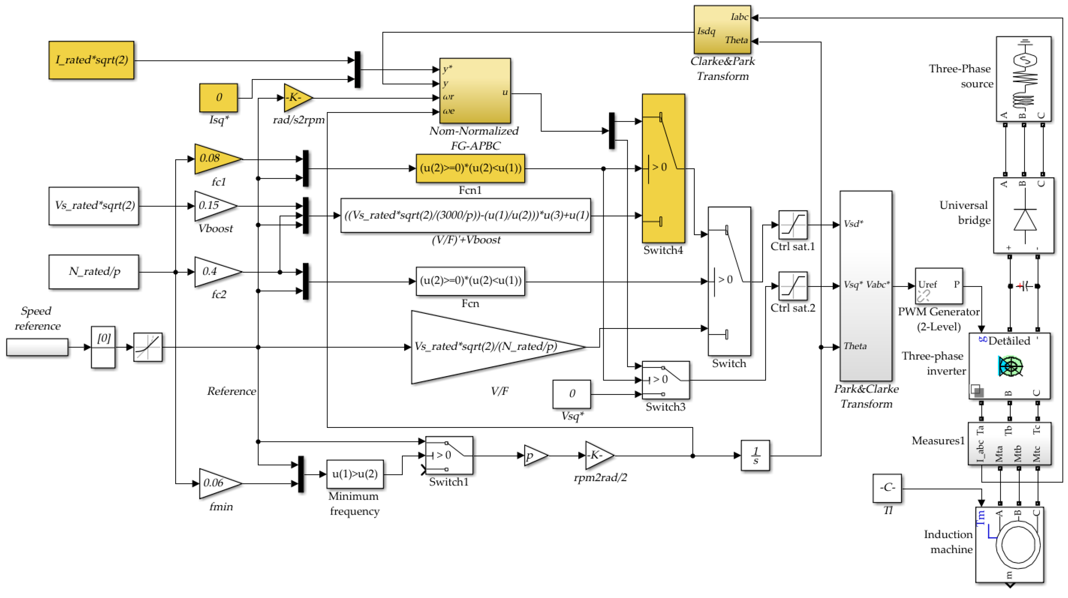
A general diagram of the proposed HST-SCS is shown in Figure 2. Here, a new HST control loop (marked in yellow) operating from the minimum frequency $f_{min}$ to the lower frequency $f_{c1}$ was added to the basic SCS. It moves the $V_{boost}$ operation from $f_{c1}$ to $f_c$, keeping the $P_2{\omega }_e^{\ast }$ operating from $f_c$ to $f_{rated}$. The new transition frequency $f_{c1}$ from HST control to $V_{boost}$ control is lower than $f_c$.

In the proposed HST-SCS, Equation (1) takes the form

$$V_s^{\ast }=\{\begin{array}{ccc}{\theta }^T\omega ,& \mathrm{with}\dot{\theta }=e{\left(\Gamma \omega \right)}^T& \mathrm{for}{f}_{min}<f<f_{c1},\\ P_1{\omega }_e^{\ast }+\sqrt{2}{V}_{boost},& \mathrm{with}{P}_1=\frac{\sqrt{2}p}{2\pi }\left(\frac{V_{s_{rated}}}{f_{rated}}-\frac{V_{boost}}{fc}\right)& \mathrm{for}{f}_{c1}<f<f_c,\\ P_2{\omega }_e^{\ast },& \mathrm{with}{P}_2=\frac{\sqrt{2}p}{2\pi }\left(\frac{V_{s_{rated}}}{f_{rated}}\right)& \mathrm{for}{f}_c<f<f_{rated},\end{array}$$

(6)

where the added HST control loop $\theta$ is the adaptive HST controller parameter, depending on the fixed-gains $\Gamma$ and the information vector $\omega$. $\theta$, $\Gamma$, and $\omega$ are all defined in Section 3.2.

3.2. Normalized FG-APBC

The APBC basis for tracking and regulation purposes is thoroughly described in [19] for nonlinear dynamical systems with unknown parameters. It will be extended in this paper for the class of nonlinear dynamical systems (4) and using a normalized FG.

Due to the characteristics of the internal dynamics z of Equation (4), Laplace transform [24] can be applied. Considering constant D and C, and assuming initial condition $z\left(0\right)$, $z\left(s\right)={\left(sI-C\right)}^{-1}D{s}^{-1}\mathrm{Y}\left(\mathrm{s}\right)+{\left(s-C\right)}^{-1}z\left(0\right)$ is obtained. Applying the final value theorem [24], i.e., $\underset{t\to \infty }{\lim }z\left(t\right)=\underset{s\to 0}{\lim }sz\left(s\right)$, we have $\underset{t\to \infty }{\lim }z=C^{-1}DY\left(s\right)$. Thus, after replacing $z=C^{-1}DY\left(s\right)$ in the terms $f_2\left(z\right)$ of Equation (4), we get that $A_1{f}_1\left(y\right)+A_2{f}_2\left(z\right)=Af\left(y\right)$, and the dynamical system (4) takes the form

$$\begin{gathered} \dot{y}=Af\left(y\right)+Bu \\ \dot{z}=Cz+Dy \end{gathered}$$

(7)

where the output variable $y\in {\Re }^n$ and the input (control) variable $u\in {\Re }^n$ are accessible. All system parameters $A\in {\Re }^{n \times m}$ and $B\in {\Re }^{n \times n}$ are unknown with B invertible, and $\tau$ is the known time constant of the system (7). It is assumed that sign(B) is known. The system function $f\left(y\right)\in {\Re }^m$ is known.

For the IM case, in Equation (7), the system function $f\left(y\right)={\left[\begin{array}{ccc}{y}^T& {\omega }_e{y}^T& \frac{p}{2}{\omega }_r{y}^T\end{array}\right]}^T\in {\Re }^6$, the system parameters are $A=\left[\begin{array}{ccc}-\frac{R_s^{\prime }}{\sigma L_s}{I}_2+\frac{R_r^2{L}_m^2}{\sigma L_s{L}_r^3}{\left[\begin{array}{cc}-\frac{R_r}{L_r}& {\omega }_{slip}\\ -{\omega }_{slip}& -\frac{R_r}{L_r}\end{array}\right]}^{-1}& \left[\begin{array}{cc}0& 1\\ -1& 0\end{array}\right]& \frac{R_r{L}_m^2}{\sigma L_s{L}_r^2}\left[\begin{array}{cc}0& 1\\ -1& 0\end{array}\right]{\left[\begin{array}{cc}-\frac{R_r}{L_r}& {\omega }_{slip}\\ -{\omega }_{slip}& -\frac{R_r}{L_r}\end{array}\right]}^{-1}\end{array}\right]$, $B=\frac{1}{\sigma L_s}{I}_2$ and $sign\left(B\right)=I_2$.

In what follows, the adaptive controller is proposed.

Theorem 1.

Let us consider the nonlinear system (7) with unknown parameters. The following adaptive controller is

$$u=\theta {\left(\Gamma \right)}^T\omega \left(K\right)\in {\Re }^n,$$

(8)

guarantees that $\underset{t\to \infty }{\lim }\left(y^{\ast }-y\right)=0$. Here, $y^{\ast }\in {\Re }^n$ is the known required output, fixed by the operator, $u\in {\Re }^n$ is the controller (8) output, applied to the system (7) input, and the controller parameters K $\in {\Re }^{+\left(n \times n\right)}$ and $\Gamma \in {\Re }^{\left(n+m\right) \times \left(n+m\right)}$ are adjusted by the designer.

Here, $\omega \in {\Re }^{\left(n+m\right)}$ is the accessible information vector given by

$$\omega ={\left[\begin{array}{cc}f{\left(y\right)}^T& {\left(Ke+{\dot{y}}^{\ast }\right)}^T\end{array}\right]}^T,$$

(9)

where K $\in {\Re }^{n \times n}$ is a Hurwitz matrix chosen by the designer as $K=\frac{1}{n\tau }$ with $\tau$ the known time constant of system (7), and ${\theta }^T\in {\Re }^{n \times \left(n+m\right)}$ are the adaptive controller parameters adjusted through the adaptive laws

$$\dot{\theta }=sign{\left(B\right)}^{T}e{\left(\Gamma \omega \right)}^T,$$

(10)

Here, the fixed-gains $\Gamma \in {\Re }^{\left(n+m\right) \times \left(n+m\right)}$ is a diagonal matrix computed according to the following normalized FG equation

$$\Gamma =\frac{\alpha I_{\left(n+m\right)}}{\left(1+{\omega }_{rated}^T{\omega }_{rated}\right)},$$

(11)

with ${\omega }_{rated}\in {\Re }^{\left(n+m\right)}$ is the rated information vector defining the operational range of $\omega$, $\alpha$ is a positive adjustable parameter chosen by the designer, and $I_{\left(n+m\right)}$ is the identity matrix of order $\left(n+m\right)$.

Proof: 

Let us define the control error as $e=y^{\ast }-y$. Subtracting ${\dot{y}}^{\ast }$ to both sides of (7), adding and subtracting the term $Ke$ in the right-hand side, and making some algebraic arrangements, it is obtained that

$$\dot{e}=-Ke+B\left({\theta }^{\ast T}\omega -u\right)$$

(12)

where ${\theta }^{\ast T}=\left[\begin{array}{cc}{B}^{-1}A& B^{-1}\end{array}\right]\in {\Re }^{n \times \left(n+m\right)}$ is the controller ideal fixed parameters of the controller, which are unknown. Substituting (8) in (12), defining the controller parameters error as $e_{\theta }={\theta }^{\ast }-\theta$ (which implies ${\dot{e}}_{\theta }=-\dot{\theta }$ as ${\theta }^{\ast }$ is constant), and considering (9), the equations describing the evolution of the errors are

$$\begin{gathered} \dot{e}=-K{e}_i+B{e}_{\theta }^T\omega \\ {\dot{e}}_{\theta }=-sign{\left(B\right)}^{T}e{\left(\Gamma \omega \right)}^T \end{gathered}$$

(13)

Let us propose the following Lyapunov candidate function, which is positive definite

$$V\left(e,e_{\theta }\right)=\frac{1}{2}{e}^{T}e+Trace{\left(\frac{1}{2}{e}_{\theta }^T{\left|B\right|}^T{e}_{\theta }{\Gamma }^{-1}\right)}_{}$$

(14)

Taking the time derivative of (14), it is obtained that $\dot{V}\left(e, e_{\theta }\right)= e^T\dot{e}+Trace\left(e_{\theta }^T{\left|B\right|}^T{\dot{e}}_{\theta }{\Gamma }^{-1}\right)$. Substituting into this last expression the derivatives of the controlled variable error $\dot{e}$ from (13) and the controller parameters error ${\dot{e}}_{\theta }$ (13), considering that ${\left(\Gamma \omega \right)}^T={\omega }^T{\Gamma }^T$, ${\Gamma }^T{\Gamma }^{-1}=1$ due to $\Gamma$ is a diagonal matrix, that $B$ equals the $sign\left(B\right)$ multiplied by $\left|B\right|$, and grouping terms, we obtain $\dot{V}\left(e, e_{\theta }\right)= -e^{T}Ke+e^{T}B{e}_{\theta }^T\omega +Trace\left(-e_{\theta }^T{B}^{T}e{\omega }^T\right)$. Now, considering the two vectors property where $a^{T}b=Trace\left(b{a}^T\right)$ to write into the trace the second term $e^{T}B{e}_{\theta }^T\omega =Trace \left(e_{\theta }^T\omega e^{T}B\right)$ and rearranging, we have $\dot{V}\left(e, e_{\theta }\right)= -e^{T}Ke+Trace\left(-e_{\theta }^T{B}^{T}e{\omega }^T+e_{\theta }^T{B}^{T}e{\omega }^T\right)$. Canceling terms allows obtaining

$$\dot{V}\left(e,e_{\theta }\right)=-e^{T}Ke\le 0$$

(15)

As can be seen in (15), the first-time derivative of the Lyapunov function (14) is negative semidefinite; thus, using Lapunov Theorem, it can be concluded that system (13) is stable.

(a)

Let us now prove that control error e converges to zero.

Integrating Equation (15) in the interval $\left(0,\infty \right)$ it is obtained that

$$V(\infty )-V\left(0\right)=-{{\displaystyle \int }}_0^{\infty }\left(e^{T}Ke\right)d\lambda$$

(16)

Since the system is stable, $e,e_{\theta }$ are all bounded ($e,e_{\theta }\in {\mathcal{L}}^{\infty }$), and from (14) it can be concluded that $\mathrm{V}$ is always bounded. Thus, the left-hand side of (16) is always bounded, which implies from the right-hand side of (16) that $e\in {\mathcal{L}}^2$.

Since $e\in {\mathcal{L}}^{\infty }$ and the reference output $y^{\ast }$ is assumed to be bounded, it can be concluded from the errors expressions that $y\in {\mathcal{L}}^{\infty }$. Thus, since $f\left(y\right)$ is assumed a bounded function for a bounded $\mathrm{y}$, from (9) $\omega \in {\mathcal{L}}^{\infty }$, and consequently, from (13), it can be concluded that $\dot{e},{\dot{e}}_{\theta }\in {\mathcal{L}}^{\infty }$.

Thus, since $e, \dot{e}\in {\mathcal{L}}^{\infty }$ and $e\in {\mathcal{L}}^2$, using Barbalat’s Lemma [18] it can be concluded that

$$\underset{t\to \infty }{\lim }e=0$$

and this concludes the proof. The controller parameters error $e_{\theta }$ is stable, and the adaptive controller parameters $\theta$ not necessarily tend to the controller ideal parameters ${\theta }^{\ast }$. □

The normalized FG-APBC for the IM is described in Figure 3, where summarizing, $u={\theta }^T\omega$, $\omega ={\left[\begin{array}{cc}\begin{array}{ccc}{y}^T& {\omega }_e{y}^T& \frac{p}{2}{\omega }_r{y}^T\end{array}& {\left(Ke+{\dot{y}}^{\ast }\right)}^T\end{array}\right]}^T\in {\Re }^8$, with $y={\left[\begin{array}{cc}{I}_{rd}& I_{rq}\end{array}\right]}^T\in {\Re }^2$, $e=\left(y^{\ast }-y\right)\in {\Re }^2$ with $y^{\ast }={\left[\begin{array}{cc}{I}_{s\_rated}& 0\end{array}\right]}^T$, $\dot{\theta }=e{\left(\Gamma \omega \right)}^T$ due to $sign{\left(B\right)}^T=1$, and $\Gamma =\frac{I_8}{\left(1+{\omega }_{rated}^T{\omega }_{rated}\right)}$ $\mathrm{with}\alpha =1\mathrm{and}$ ${\omega }_{rated}={\left[\begin{array}{ccc}{I}_{s\_rated}& 0& \begin{array}{ccc}2\pi f_{rated}{I}_{s\_rated}& 0& \begin{array}{ccc}\frac{p}{2}{\omega }_{r\_rated}{I}_{s\_rated}& 0& \begin{array}{cc}0& 0\end{array}\end{array}\end{array}\end{array}\right]}^T$. The value $K=50/J_m$ is chosen, with $J_m$ the motor inertia taken from the IM datasheet. The value $K=\frac{50}{J_m}=\frac{1}{(J_m/\left(10\times 5\right)}$ came from the widely used criterion considering the inner current loop 10 as times faster than the outer mechanical loop and our proposal for the normalized FG-APBC of considering a controller time as a constant of a fifth the inner time constant of the plant.

In order to verify the achievement of the proposal goal, comparative experimental results considering real-time simulations are described in the next section.

4. Experimental Comparative Results and Discussion

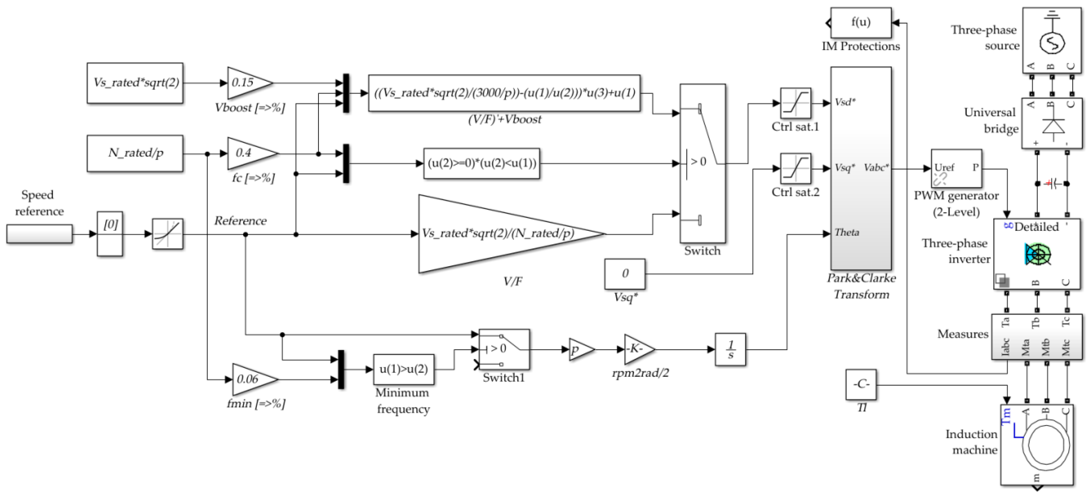
The schemes from Figure 1 (basic SCS) and Figure 2 (proposed HST-SCS) were applied to an IM of 200 HP. These were programmed in Simulink version 8.9 of Matlab R2017a (9.2.0.538062) for Win64. Later, they were downloaded into a real-time simulator controller 4510 v2 from OPAL-RT and run. The field-programmable gate array (FPGA) of the OPAL was used to creates a hardware implementation of portions of the software application.

The real-time simulations started at 0 s and stopped at 35 s using a sampling time of 10 μs. In both cases, a constant speed setpoint was applied equal to the nominal speed value and a ramp of 50 rpm/s.

The inverter trip unit was running at the FPGA of the controller and works at 2 kHz. The motor data plate is 149.2 kW, 460 V, 60 Hz, 1755 rpm (183.8 rad/s), fp = 0.85, η = 86.6%, T_nom = 812 Nm, and the motor inertia taken from its datasheet is 3.1 Kgm². The parameters of the motor-load set (considered unknown) are p = 4, L_m = 10.46 mH, L_s = L_r = 10.7627 mH, R_s = 14.85 mΩ, R_r = 9.295 mΩ, J = 6.2 Kgm², and B = 0.08 Nms.

4.1. Basic SCS

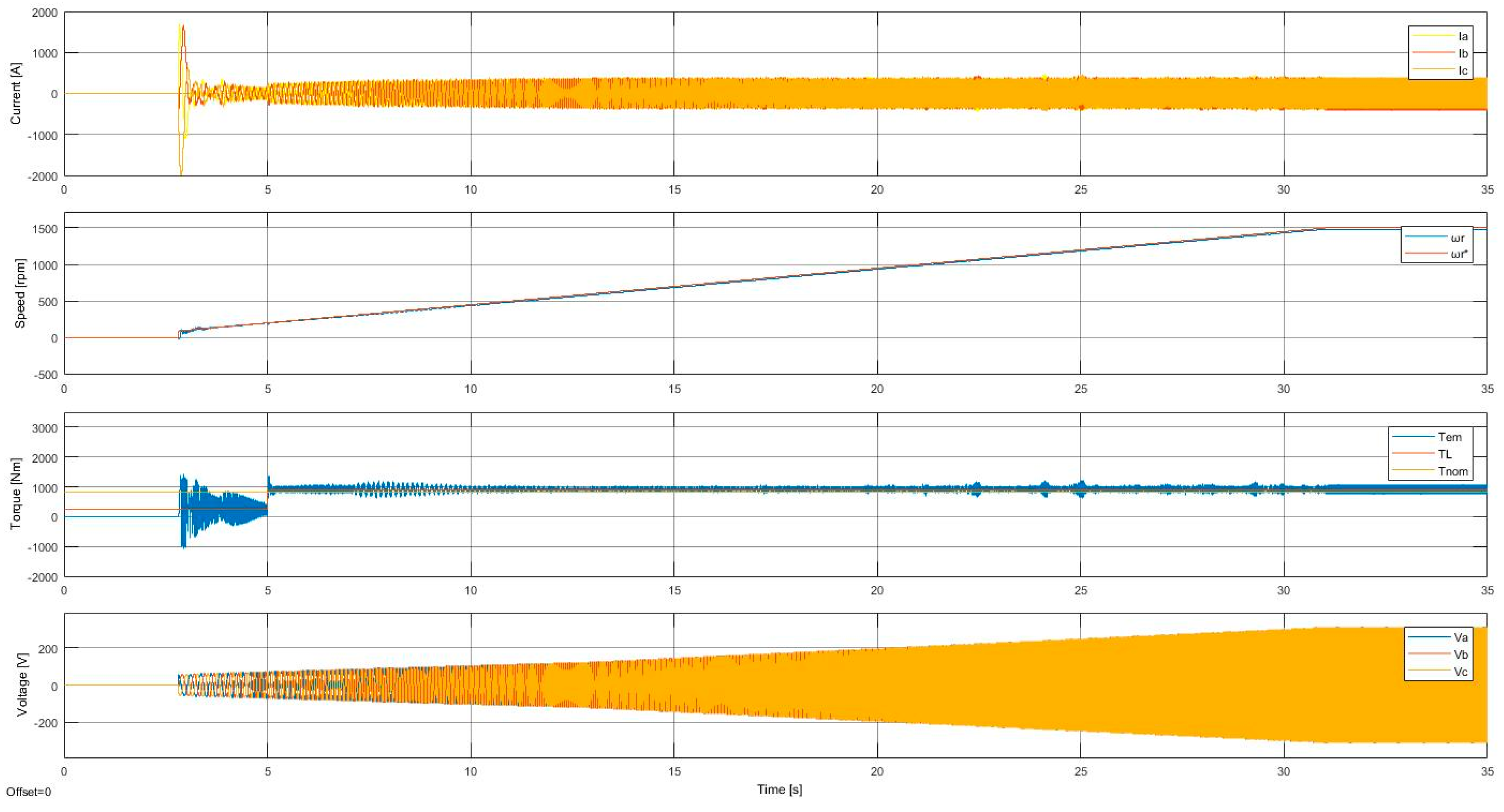
In this case, the following SCS configuration parameters were used: $V_{s\_rated}=460/\sqrt{3}$, $f_{rated}=60\mathrm{Hz}$, $f_c=40\%f_{rated}$, $V_{boost}=15\%V_{s\_rated}$, and $f_{min}=6\% f_{rated}$. The experimental results for a starting torque T_l = 30% T_nom, increasing to 110% T_nom at 5 s, are shown in Figure 4.

Figure 4 shows the results of the basic SCS, starting with 30% of the nominal torque. The slope of the voltage amplitude decreased at a time between 15 and 20 s at 40% of the required speed. A torque ripple is shown at low speeds. The real rotor speed followed the required rotor with an accuracy of 2.2%.

There is a smooth change when switching the voltage in Equation (1) at the frequency $f_c$. Neither the rotor speed, the stator current, nor the torque is affected by this change of the control method.

4.2. Proposed Adaptive HST-SCS

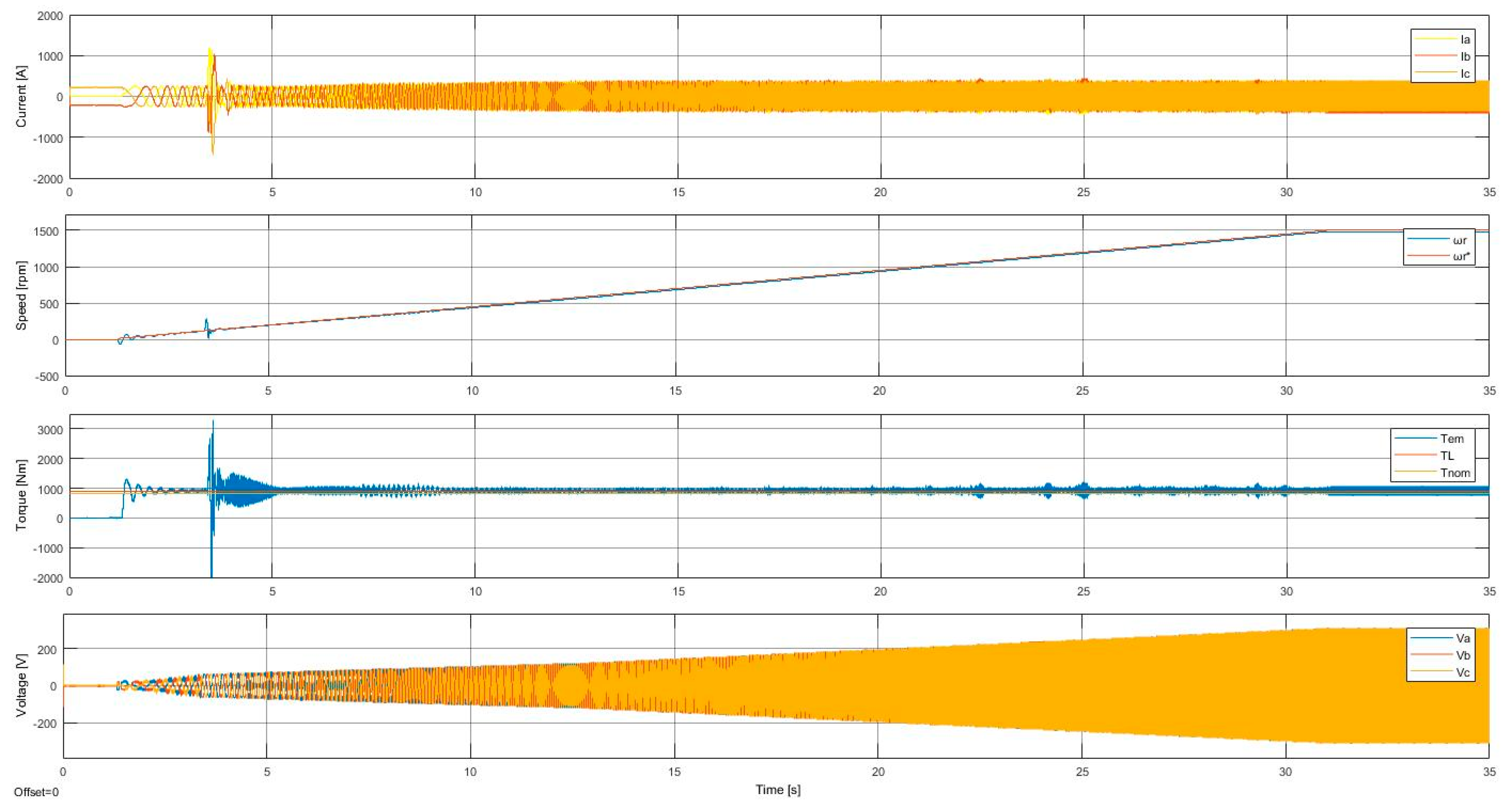
The SCS configuration parameters in this case were the same used by the basic SCS ($V_{s\_rated}=460/\sqrt{3}$, $f_{rated}=60\mathrm{Hz}$, $f_c=40\% f_{rated}$, $V_{boost}=15\% V_{s\_rated}$, and $f_{min}=1\%f_{rated}$), and additionally, $f_{c1}=8\%f_{rated}$, $I_{s\_rated}=255A$, $\Gamma =\frac{I_v}{\left(1+{\omega }_{rated}^T{\omega }_{rated}\right)}$, and $J_m=3.1{\mathrm{kgm}}^2$. The experimental results are shown in Figure 5.

Results from Figure 5 show the achievement of the proposed goal after starting with 110% of the nominal torque. Conversely to the basic SCS results from Figure 4, the HST-SCS is characterized by having the motor magnetized from zero speed consuming the rated stator current. It has a higher voltage slope after starting. It also consumes a starting stator current smaller than the basic SCS loaded with 30% of the nominal torque (see Figure 4). After $f_{c1}$, the HST-SCS behaves like the basic SCS: the slope of the voltage amplitude decreased at a time between 15 to 20 s at 40% of the required speed; a torque ripple is also shown at low speeds, and the real rotor speed followed the required rotor with an accurate of 2.2%.

Distinctly from the basic SCS (Figure 4), the HST-SCS (Figure 5) shows an extra change in the slope of the voltage amplitude. It is higher at a time between 3 and 4 s at 8% of the required speed. At this point, the control strategy changes from the HST-SCS to the SCS, showing higher torque amplitude in correspondence to the higher torque load. The exact switching point fixed at 8% could change, looking for a smoother strategy change.

When switching between its control methods, the rotor speed, the stator current, and the torque shown in Figure 5 are affected in the HST-SCS. In particular, there is a torque ripple caused by the algorithm switching which is higher than for the basic SCS (Figure 4). This is a disadvantage of the HST-SCS over the basic SCS that should be improved in future work.

5. Conclusions

An HST-SCS for IM was proposed based on the basic SCS. The proposed SCS considers an adaptive current controller based on a direct APBC scheme using a normalized FG to fine-tune the adaptive controller parameter that works without the knowledge of the motor-load parameters. The main advantages of the HST-SCS include the capability to move higher starting-torque loads, together with a simple and cost-effective implementation without needing a rotor speed sensor or estimator, variable observers, or parameter estimators. The basic SCS for IM and the HST-SCS were applied to an IM of 200 HP and tested using the real-time simulator controller 4510 v2 from OPAL-RT. The HST-SCS started with 110% of the nominal torque, consuming less stator current than the basic SCS with a load torque of 30% of the nominal torque. Besides the rated voltage per phase needed by the basic SCS, the proposed HST-SCS needs the rated current per phase and motor inertia taken from the IM datasheet.

There is a torque ripple caused by the algorithm-switching of the HST-SCS, which is higher than for the basic SCS starting. This is a disadvantage of the HST-SCS over the basic SCS, which has a smooth change between its methods. Neither the rotor speed, the stator current, nor the torque is affected by this change of the control method in the basic SCS.

In future work, the proposed HST-SCS should be validated under a small scale test bench. In addition, using a motor of low rated power, the torque ripple magnitude, increased during the switching between methods, should be studied and decreased as much as possible.

References

1. Hannan, M.A.; Jamal, A.A.; Mohamed, A.; Hussain, A. Optimization techniques to enhance the performance of induction motor drives: A review. Renew. Sustain. Energy Rev. 2017, 81, 1611–1626. [Google Scholar] [CrossRef]
2. Peter, V. Sensorless Vector and Direct Torque Control; Oxford University Press: Oxford, UK, 1998. [Google Scholar]
3. Bose, B.K. Modern Power Electronics and AC Drives; Prentice Hall PTR: Upper Saddle River, NJ, USA, 2002. [Google Scholar]
4. Depenbrock, M. Direkte Selbstregelung (DSR) fiir hochdynamische Drehfeld-antriebe mit Stromrichterschaltung. Etz Arch. 1985, 7, 211–218. [Google Scholar]
5. Hasse, K. Zur Dynamik Drehzahlgeregelter Antriebe Mit Stromrichtergespeisten Asynchron-Kurzschlussläufer Maschinen. Ph.D. Thesis, Technical University of Darmstadt, Darmstadt, Germany, 1969. [Google Scholar]
6. Blaschke, F. The principle of field orientation as Applied to the New “transvektor” Close–loop Control system for Rotating-Field machines. Siemens Rev. 1972, 39, 517–525. [Google Scholar]
7. Karbakhsh, F.; Amiri, M.; Zarchi, H.A. Two-switch flyback inverter employing a current sensorless MPPT and scalar control for low cost solar powered pumps. IET Renew. Power Gener. 2017, 11, 669–677. [Google Scholar]
8. Krein, P.T.; Disilvestro, F.; Kanellakopoulos, I.; Locker, J. Comparative analysis of scalar and vector control methods for induction motors. In Proceedings of the IEEE Power Electronics Specialist Conference-PESC ‘93, Seattle, WA, USA, 20–24 June 1993; pp. 1139–1145. [Google Scholar] [CrossRef]
9. García, G.O.; Stephan, R.M.; Watanabe, E.H. Comparing the Indirect Field-Oriented Control with a Scalar Method. IEEE Trans. Ind. Electron. 1994, 41, 201–207. [Google Scholar]
10. Papazian, J.C.; Rognon, J.P.; Roye, D.; Delbosc, P. From scalar control to space vector control: Functions and limitations of the different elements. In Proceedings of the IAS ’95. Conference Record of the 1995 IEEE Industry Applications Conference Thirtieth IAS Annual Meeting, Orlando, FL, USA, 8–12 October 1995; Volume 3, pp. 1944–1950. [Google Scholar] [CrossRef]
11. Ueda, R.; Sonoda, T.; Koga, K.; Ichikawa, M. Stability Analysis in Induction-Motor Driven by V/F Controlled General-Purpose Inverter. IEEE Trans. Ind. Appl. 1992, 28, 472–481. [Google Scholar]
12. Koga, K.; Ueda, R.; Sonoda, T. Constitution of V/F Control for Reducing the Steady-State Speed Error to Zero in Induction-Motor Drive System. IEEE Trans. Ind. Appl. 1992, 28, 463–471. [Google Scholar]
13. Munoz-García, A.; Lipo, T.A.; Novotny, D.W. A new induction motor V/f control method capable of high-performance regulation at low speeds. IEEE Trans. Ind. Appl. 1998, 34, 813–821. [Google Scholar]
14. Wang, C.C.; Fang, C.H. Sensorless scalar-controlled induction motor drives with modified flux observer. IEEE Trans. Energy Convers. 2003, 18, 181–186. [Google Scholar]
15. Smith, A.; Gadoue, S.; Armstrong, M.; Finch, J. Improved method for the scalar control of induction motor drives. IET Electr. Power Appl. 2013, 7, 487–498. [Google Scholar]
16. Suetake, M.; da Silva, I.N.; Goedtel, A. Embedded DSP-Based Compact Fuzzy System and Its Application for Induction-Motor V/f Speed Control. IEEE Trans. Ind. Electron. 2011, 58, 750–760. [Google Scholar]
17. Tshiloz, K.; Djurović, S. Scalar controlled induction motor drive speed estimation by adaptive sliding window search of the power signal. Int. J. Electr. Power Energy Syst. 2017, 91, 80–91. [Google Scholar]
18. Narendra, K.S.; Annaswamy, A.M. Stable Adaptive Systems; Dovers publications: Mineola, NY, USA, 2005. [Google Scholar]
19. Travieso-Torres, J.C.; Duarte-Mermoud, M.A.; Sepuleveda, D.I. Passivity-based control for stabilization, regulation and tracking purposes of a class of nonlinear systems. Int. J. Adapt. Control Signal Process. 2017, 21, 582–602. [Google Scholar] [CrossRef]
20. Vas, P. Electrical Machines and Drives: Space Vector Theory Approach; Editorial Oxford Clarendon Press: Oxford, UK, 1992. [Google Scholar]
21. Control Techniques Drives Limited. Commander SE Advanced User Guide; Control Techniques Drives Limited: Hong Kong, China, 2002. [Google Scholar]
22. Park, R.H. Two-Reaction Theory of Synchronous Machines, Generalized Method of Analysis-Part I. Trans. Am. Inst. Electr. Eng. 1929, 48, 716–730. [Google Scholar] [CrossRef]
23. Mandic, D.P.; Kanna, S.; Xia, Y.L.; Moniri, A.; Junyent-Ferre, A.; Constantinides, A.G. A Data Analytics Perspective of Power Grid Analysis-Part 1: The Clarke and Related Transforms. IEEE Signal Process. Mag. 2019, 36, 110–116. [Google Scholar] [CrossRef]
24. Schiff, J.L. The Laplace Transform: Theory and Applications; Springer: Berlin/Heidelberg, Germany, 1999; ISBN 0387986987. [Google Scholar]
Figure 1. Simulink block diagram of basic SCS for the induction motor (IM).
Energies 13 01276 g001
Figure 2. Simulink block diagram of the proposed HST-SCS for the IM.
Energies 13 01276 g002
Figure 3. Simulink block diagram of the normalized FG-APBC for the IM.
Energies 13 01276 g003
Figure 4. Real-time simulation results of the basic SCS for a 200 HP IM.
Energies 13 01276 g004
Figure 5. Real-time simulation results of the proposed adaptive HST-SCS for a 200 HP IM.
Energies 13 01276 g005