Optimized Scheduling of EV Charging in Solar Parking Lots for Local Peak Reduction under EV Demand Uncertainty


Abstract
1. Introduction
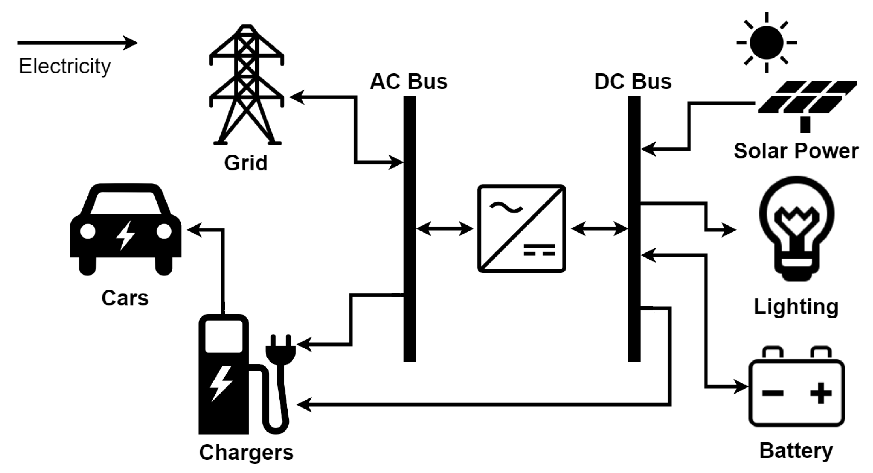
2. System Description
2.1. Solar Parking Lots
2.2. Batteries
2.3. Electric Vehicle Supply Equipment
2.4. Electric Vehicle Load Profile
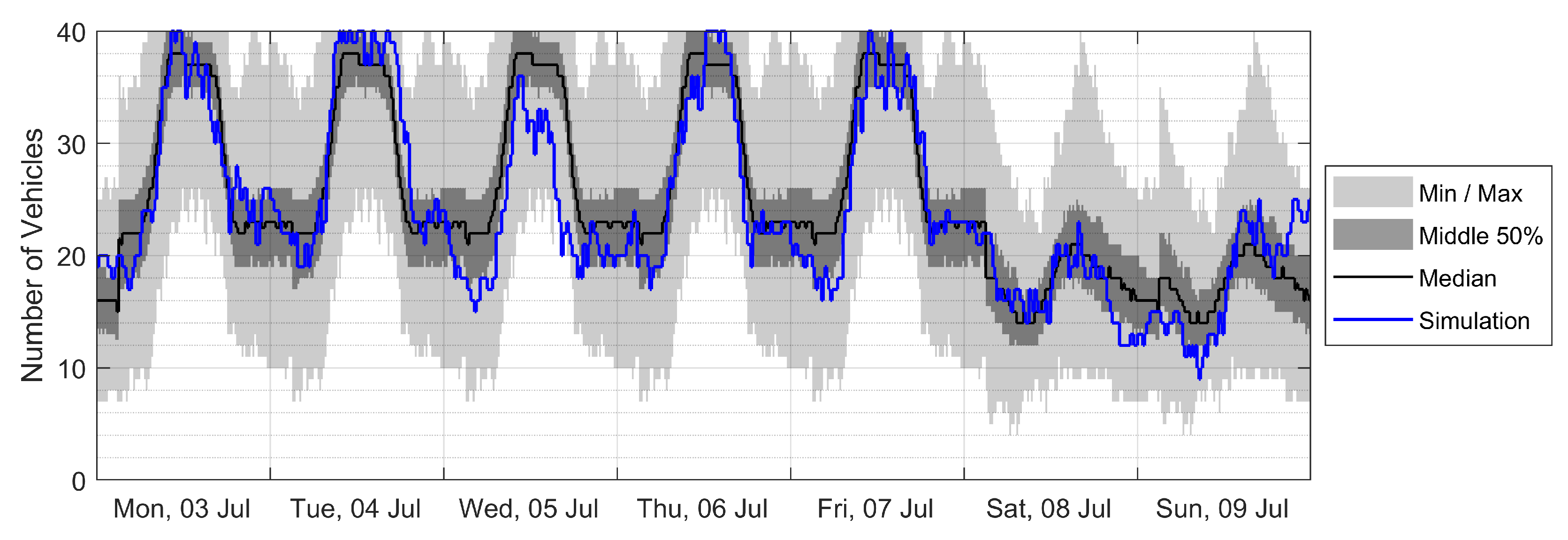
2.4.1. EV Arrival and Departure
2.4.2. EV State of Charge on Arrival
3. Methods for Charge Scheduling
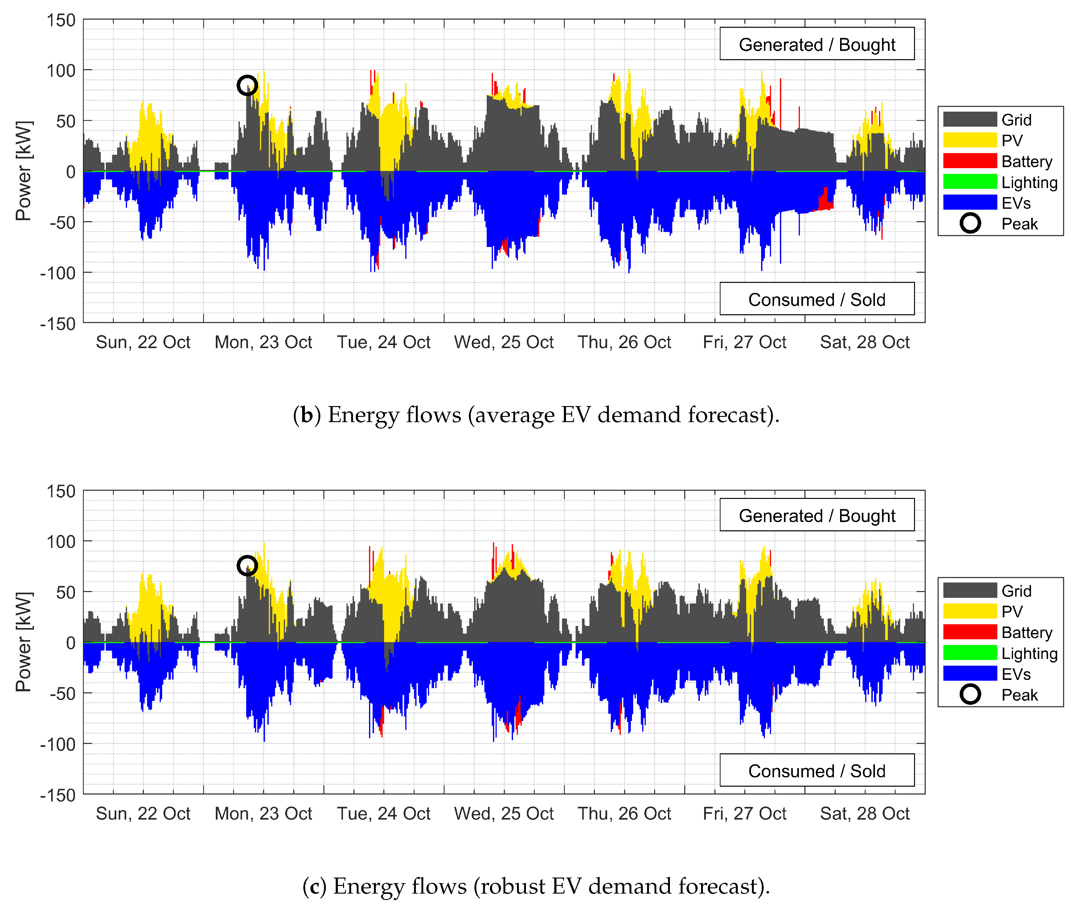
- No EV demand forecast: EV charging is scheduled without a forecast of energy demand for EVs arriving in the future
- Average EV demand forecast: EV charging is scheduled with a single forecast of energy demand for EVs arriving in the future which is based on average values.
- Robust EV demand forecast: EV charging is scheduled to be robust across a range of possible energy demands for EVs arriving in the future
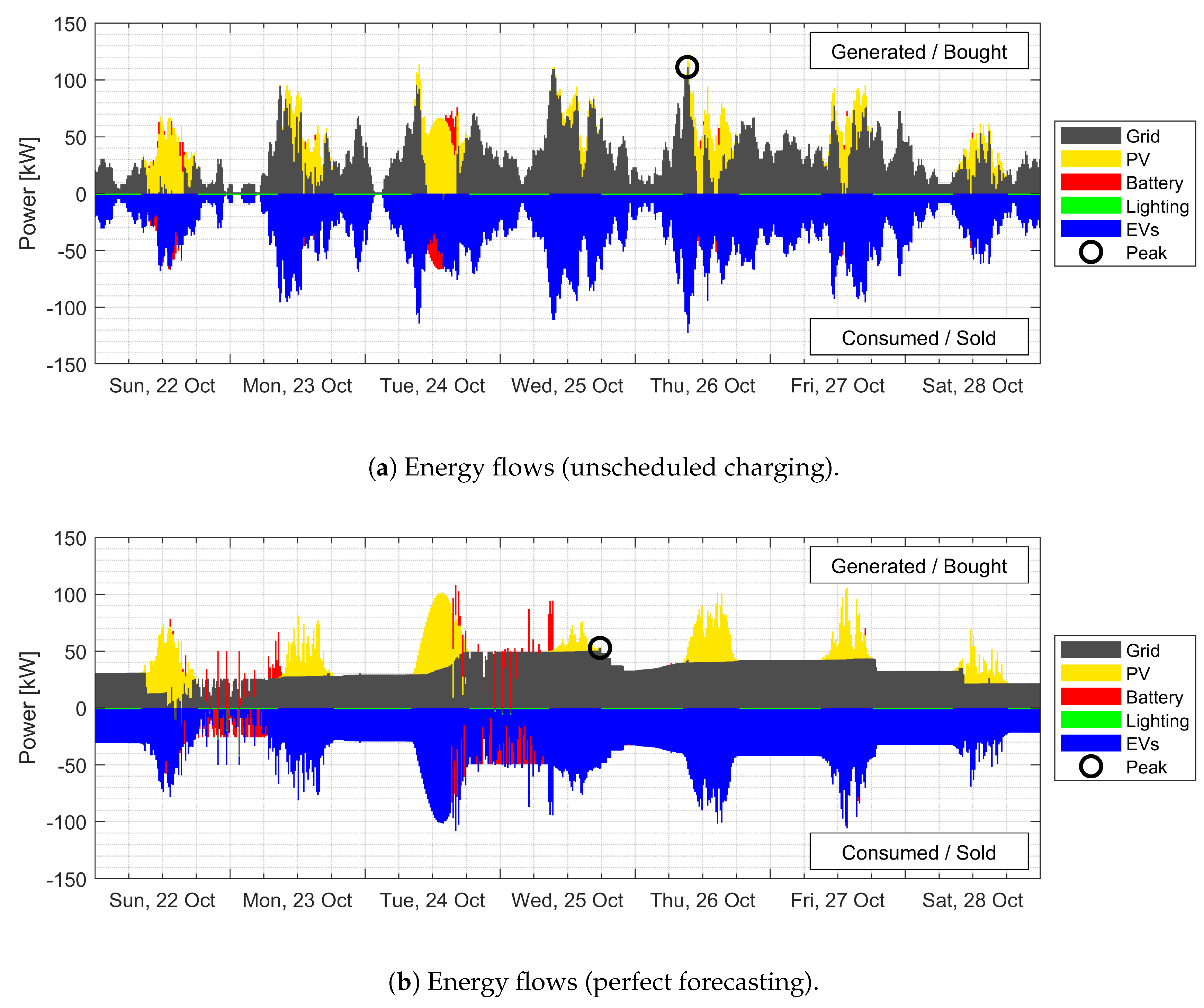
3.1. Problem Formulation with Perfect Forecasting
3.2. Inclusion of Uncertainty in Forecasting
3.2.1. Uncertainty in PV Forecasting
3.2.2. Uncertainty in EV Forecasting
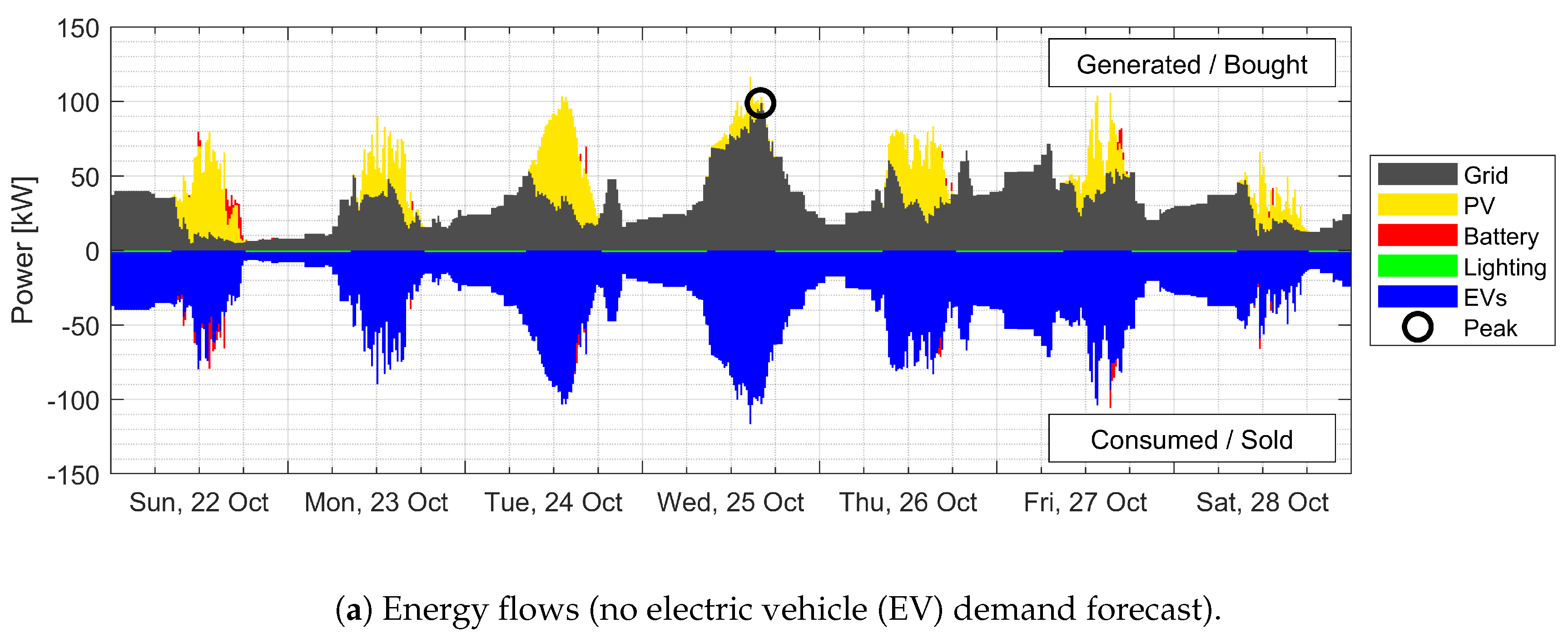
3.3. No EV Demand Forecast
3.4. Average EV Demand Forecast
3.5. Robust EV Demand Forecast
4. Results and Discussion
4.1. Example Simulations
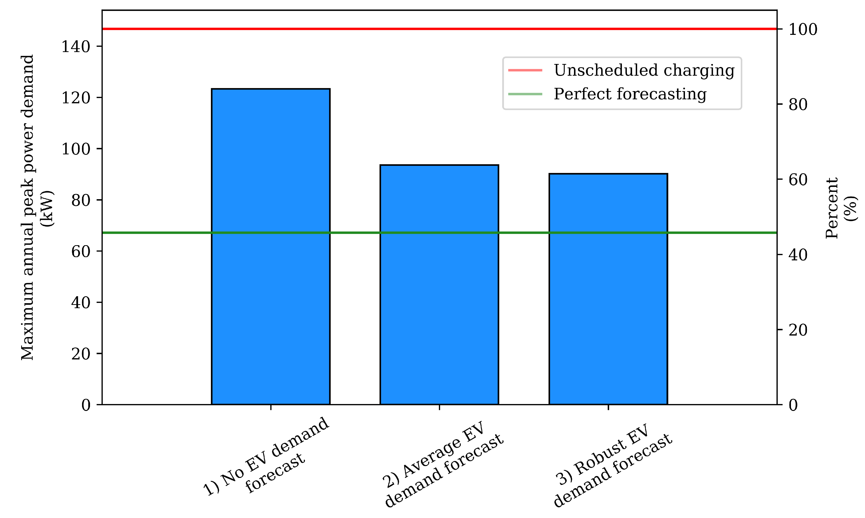
4.2. Maximum Annual Peak Exchange with the Grid
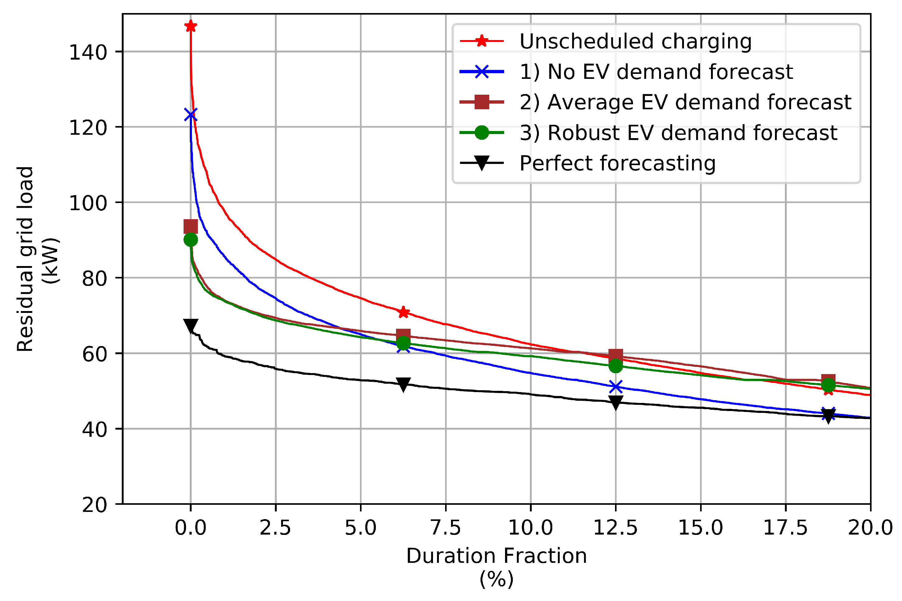
4.3. Duration of Peak Loads
5. Conclusions
- No EV demand forecast: EV charging is scheduled without a forecast of energy demand for EVs arriving in the future
- Average EV demand forecast: EV charging is scheduled with a single forecast of energy demand for EVs arriving in the future which is based on average values.
- Robust EV demand forecast: EV charging is scheduled to be robust across a range of possible energy demands for EVs arriving in the future
Author Contributions
Funding
Acknowledgments
Conflicts of Interest
List of Symbols
| Symbol | Definition | Unit | Note |
| Forecasted PV generation: | kWh | ||
| kWh | |||
| Max energy that can be sent to the grid | kWh | 32 kWh = 120 kW | |
| Grid exchange: | kWh | ||
| Energy to (+) or from (-) battery i at time t | kWh | ||
| Load from lighting at time t | kWh | ||
| Generation from solar power at time t | kWh | ||
| i | Index for each battery, 1–40 = EVs, 41 = fixed storage | - | |
| k | Current time step | - | |
| Max possible value of | kWh | ||
| Min possible value of : | kWh | ||
| Total number of batteries | - | 41 = 40 EVs + 1 battery | |
| Number of errors in the bounded set | - | 10,000 | |
| Number of time steps in MPC time horizon | - | ||
| Number of time steps in one full simulation | - | 34,944 = 24 · 4 · 364 | |
| Maximum power to or from battery i | kW | EVs 7.4 kW, battery 50 kW | |
| Energy stored in battery i at time t | kWh | ||
| Maximum energy allowed in battery i at time t | kWh | ||
| Minimum energy allowed in battery i at time t | kWh | ||
| Average value for the max energy in battery i at time t | kWh | ||
| Average value for the min energy in battery i at time t | kWh | ||
| t | time step within MPC horizon | - | |
| kWh | |||
| Length of a single time step | h | 15 min = 0.25 h | |
| For battery i at time t: 0 if discharging, 1 if charging | |||
| Charging efficiency of battery i | - | ||
| Discharging efficiency of battery i | - | ||
| Bounded set of PV forecasting errors | - | ||
| PV forecasting error at time t | kWh | ||
| Max PV forecasting error in set | kWh | ||
| Min PV forecasting error in the set | kWh | ||
| Uncertainty in the value of | kWh | ||
| Uncertainty in the value of | kWh |
References
- Olivier, J.; Schure, K.; Peters, J. Trends in Global CO2 and Total Greenhouse Gas Emissions—2017 Report; Technical Report 2674; PBL Netherlands Environmental Assessment Agency: The Hague, The Netherlands, 2017. [Google Scholar]
- Van Mierlo, J.; Messagie, M.; Rangaraju, S. Comparative environmental assessment of alternative fueled vehicles using a life cycle assessment. Transp. Res. Procedia 2017, 25, 3435–3445. [Google Scholar] [CrossRef]
- Van Vliet, O.; Brouwer, A.S.; Kuramochi, T.; van den Broek, M.; Faaij, A. Energy use, cost and CO2 emissions of electric cars. J. Power Sources 2011, 196, 2298–2310. [Google Scholar] [CrossRef]
- Dubey, A.; Santoso, S. Electric Vehicle Charging on Residential Distribution Systems: Impacts and Mitigations. IEEE Access 2015, 3, 1871–1893. [Google Scholar] [CrossRef]
- Verzijlbergh, R.A.; Lukszo, Z.; Slootweg, J.G.; Ilic, M.D. The impact of controlled electric vehicle charging on residential low voltage networks. In Proceedings of the 2011 International Conference on Networking, Sensing and Control, Delft, The Netherlands, 11–13 April 2011; pp. 14–19. [Google Scholar] [CrossRef]
- Uddin, M.; Romlie, M.F.; Abdullah, M.F.; Abd Halim, S.; Abu Bakar, A.H.; Chia Kwang, T. A review on peak load shaving strategies. Renew. Sustain. Energy Rev. 2018, 82, 3323–3332. [Google Scholar] [CrossRef]
- Verzijlbergh, R.A.; De Vries, L.J.; Lukszo, Z. Renewable Energy Sources and Responsive Demand. Do We Need Congestion Management in the Distribution Grid? IEEE Trans. Power Syst. 2014, 29, 2119–2128. [Google Scholar] [CrossRef]
- Clement-Nyns, K.; Haesen, E.; Driesen, J. The Impact of Charging Plug-In Hybrid Electric Vehicles on a Residential Distribution Grid. IEEE Trans. Power Syst. 2010, 25, 371–380. [Google Scholar] [CrossRef]
- PricewaterhouseCoopers. Smart Charging of Electric Vehicles: Institutional Bottlenecks and Possible Solutions; Technical Report; PricewaterhouseCoopers: Utrecht, The Netherlands, 2017. [Google Scholar]
- Sortomme, E.; El-Sharkawi, M.A. Optimal Scheduling of Vehicle-to-Grid Energy and Ancillary Services. IEEE Trans. Smart Grid 2012, 3, 351–359. [Google Scholar] [CrossRef]
- Van der Kam, M.; van Sark, W. Smart charging of electric vehicles with photovoltaic power and vehicle-to-grid technology in a microgrid: A case study. Appl. Energy 2015, 152, 20–30. [Google Scholar] [CrossRef]
- Sarantis, I.; Alavi, F.; Schutter, B.D. Optimal power scheduling of fuel-cell-car-based microgrids. In Proceedings of the 2017 IEEE 56th Annual Conference on Decision and Control (CDC), Melbourne, Australia, 12–15 December 2017; pp. 5062–5067. [Google Scholar] [CrossRef]
- Knap, W. Horizon at Station Cabauw; Pangaea: Cabauw, The Netherlands, 2007. [Google Scholar] [CrossRef]
- Stein, J.S.; Holmgren, W.F.; Forbess, J.; Hansen, C.W. PVLIB: Open source photovoltaic performance modeling functions for Matlab and Python. In Proceedings of the 2016 IEEE 43rd Photovoltaic Specialists Conference (PVSC), Portland, OR, USA, 5–10 June 2016; pp. 3425–3430. [Google Scholar] [CrossRef]
- Apostolaki-Iosifidou, E.; Codani, P.; Kempton, W. Measurement of power loss during electric vehicle charging and discharging. Energy 2017, 127, 730–742. [Google Scholar] [CrossRef]
- Shareef, H.; Islam, M.M.; Mohamed, A. A review of the stage-of-the-art charging technologies, placement methodologies, and impacts of electric vehicles. Renew. Sustain. Energy Rev. 2016, 64, 403–420. [Google Scholar] [CrossRef]
- Daina, N.; Sivakumar, A.; Polak, J.W. Modelling electric vehicles use: A survey on the methods. Renew. Sustain. Energy Rev. 2017, 68, 447–460. [Google Scholar] [CrossRef]
- Francfort, J. EV Project Data & Analytic Results; Idaho National Laboratory: Idaho Falls, ID, USA, 2014. [Google Scholar]
- Bemporad, A.; Morari, M. Robust model predictive control: A survey. In Robustness in Identification and Control; Garulli, A., Tesi, A., Eds.; Lecture Notes in Control and Information Sciences; Springer: London, UK, 1999; pp. 207–226. [Google Scholar]
- Bemporad, A.; Morari, M. Control of systems integrating logic, dynamics, and constraints. Automatica 1999, 35, 407–427. [Google Scholar] [CrossRef]
- IEEE. C57.91-2011—IEEE Guide for Loading Mineral-Oil-Immersed Transformers and Step-Voltage Regulators; IEEE: Piscataway, NJ, USA, 2012; pp. 1–123. Available online: https://ieeexplore.ieee.org/document/6166928 (accessed on 18 November 2019). [CrossRef]
- Smith, M.; Castellano, J. Costs Associated with Non-Residential Electric Vehicle Supply Equipment: Factors to Consider in the Implementation of Electric Vehicle Charging Stations; Technical Report DOE/EE-1289; U.S. Department of Energy Vehicle Technologies Office: Washington, DC, USA, 2015.
- Blok, R.F.P. Verslag Benchmark Publiek Laden 2018—Sneller naar een Volwassen Markt; Technical Report; NKL Nederland: Emmen, NL, USA, 2018. [Google Scholar]


| Characteristic | Value |
|---|---|
| Module technology | Monocrystalline silicon |
| Module rated power | 300 kWp (60 cell) |
| Module rated efficiency | 18.33% at STC |
| Array installed capacity | 120 kWp |
| Site latitude | 5158′ N |
| Site longitude | 455′ E |
| Array azimuth | 0 (South) |
| Array tilt | 13 |
| Parking spaces | 40 spaces |
| Carport roof topology | Monopitch (single tilt angle for entire roof) |
| Annual production (DC) | 133,625 kWh |
| Capacity factor (DC) | 12.7% |
| EV Type | Mean | Standard Deviation | Lower Bound | Upper Bound |
|---|---|---|---|---|
| BEV | 50% | 18% | 0% | 90% |
| PHEV | 45% | 30% | 0% | 90% |
| Nr. | Scenario | Annual Peak Power (kW) | Relative Peak Reduction (%) |
|---|---|---|---|
| Ref | Unscheduled charging | 147 | 0% |
| 1 | No EV forecast | 123 | 16% (↓) |
| 2 | Average EV forecast | 94 | 36% (↓) |
| 3 | Robust EV forecast | 90 | 39% (↓) |
| Ref | Perfect forecasting | 67 | 54% (↓) |
© 2020 by the authors. Licensee MDPI, Basel, Switzerland. This article is an open access article distributed under the terms and conditions of the Creative Commons Attribution (CC BY) license (http://creativecommons.org/licenses/by/4.0/).
Share and Cite
Ghotge, R.; Snow, Y.; Farahani, S.; Lukszo, Z.; van Wijk, A. Optimized Scheduling of EV Charging in Solar Parking Lots for Local Peak Reduction under EV Demand Uncertainty. Energies 2020, 13, 1275. https://doi.org/10.3390/en13051275
Ghotge R, Snow Y, Farahani S, Lukszo Z, van Wijk A. Optimized Scheduling of EV Charging in Solar Parking Lots for Local Peak Reduction under EV Demand Uncertainty. Energies. 2020; 13(5):1275. https://doi.org/10.3390/en13051275
Chicago/Turabian StyleGhotge, Rishabh, Yitzhak Snow, Samira Farahani, Zofia Lukszo, and Ad van Wijk. 2020. "Optimized Scheduling of EV Charging in Solar Parking Lots for Local Peak Reduction under EV Demand Uncertainty" Energies 13, no. 5: 1275. https://doi.org/10.3390/en13051275
APA StyleGhotge, R., Snow, Y., Farahani, S., Lukszo, Z., & van Wijk, A. (2020). Optimized Scheduling of EV Charging in Solar Parking Lots for Local Peak Reduction under EV Demand Uncertainty. Energies, 13(5), 1275. https://doi.org/10.3390/en13051275