Control of a Modular Multilevel Matrix Converter for Unified Power Flow Controller Applications

Abstract

The modular multilevel matrix converter has been proposed as a suitable option for high power applications such as flexible AC transmission systems. Among flexible AC transmission systems, the unified power flow controller stands out as the most versatile device. However, the application of the modular multilevel matrix converter has not been thoroughly analyzed for unified power flow controller applications due to the sophisticated control systems that are needed when its ports operate at equal frequencies. In this context, this paper presents a cascaded control structure for a modular multilevel matrix converter based unified power flow controller. The control is implemented in a decoupled reference frame, and it features proportional-integral external controllers and internal proportional multi-resonant controllers. Additionally, the input port of the modular multilevel matrix converter is regulated in grid-feeding mode, and the output port is regulated in grid-forming mode to provide power flow compensation. The effectiveness of the proposed vector control system is demonstrated through simulation studies and experimental validation tests conducted with a 27-cell 5 kW prototype.

1. Introduction

In recent years, a series of power quality problems, such as harmonic distortion, voltage swells and sags, and current harmonics, have been arising in power grids due to the development of large-scale applications of non-linear loads, as well as mass integration of renewable energy generation. The increase of power quality problems might have an adverse impact on steady state and dynamic stability, limited transmission capacity, and congestion of lines. Therefore, Flexible Alternating Current Transmission Systems (FACTS) have been widely used to improve power grid dynamic and static behavior, providing greater operating flexibility and better utilization [1].

Depending on the technology and their connection to the grid, FACTS are classified as shunt, series, and combined devices [2]. Shunt FACTS, such as the Static Var Compensator (SVC) or the Static Synchronous Compensator (STATCOM), allow transmission line relief, power factor correction, and voltage control [3]. On the other hand, series control FACTS devices, such as the Series Static Synchronous Compensator (SSSC), imply a series voltage injection in the transmission line allowing reactive and active power compensation depending on the phase voltage, impedance line control, and transmission line relief [4]. Finally, combined control FACTS refers to the connection of series-series or series-parallel FACTS [2], as shown in Figure 1a. For instance, the Unified Power Flow Controller (UPFC) is a combined control FACTS with the capability of bidirectional power flow control, voltage and reactive power control, as well as improving the steady and dynamic stability of power grids [3,4].

As UPFC devices are rated at high-power ratios, thyristor based UPFC has been the preferred technology [5]. Despite the high efficiency and high-power operation capability, thyristor based UPFC presents several drawbacks, such as high harmonic distortion, low switching frequency operation, and reduced controllability. Consequently, Modular Multilevel Cascaded Converters (MMCC) have emerged as suitable alternatives for UPFC applications, due to their characteristics such as high efficiency, high power quality, full modularity, easy extendibility to reach high voltage levels, redundancy, control flexibility, and power quality [6,7].

Recently, the use of MMCC for UPFC applications has been validated in research and industrial projects. The Modular Multilevel Converter ($M^{2}C$) and the Modular Multilevel Matrix Converter ($M^{3}C$) are the most studied topologies [7,8]. The $M^{2}C$ has been extensively used for High-Voltage Direct Current (HVDC) transmission [9,10], STATCOM, and UPFC applications [11,12,13]. On the other hand, the $M^{3}C$ has been proposed for wind energy [14,15,16,17], grid interconnection [18,19,20], drives [20,21,22,23], and UPFC applications [24,25].

As shown in Figure 1b, the $M^{3}C$ is composed of nine clusters based on series-connected full-bridge cells. The main control challenge in this converter is the regulation of the floating capacitor voltages, which might become complex when the input/output frequencies are similar/identical because large capacitor voltage oscillations can be produced [8]. Cascaded control systems based on decoupled modeling of the $M^{3}C$ have been proposed to decouple the converter voltages and currents, simplifying the control of circulating currents and common-mode voltage [21,22]. Additionally, the operating range of the $M^{3}C$ is usually divided into two modes: the Different Frequencies Mode (DFM) and the Equal Frequencies Mode (EFM). The DFM is enabled when the input-port frequency is different from the output-port frequency, and the capacitor voltage mean values are controlled to keep proper capacitor voltage balancing. On the other hand, the EFM is enabled when the absolute value of the input-port frequency is very close or equal to the output-port frequency. In this case, circulating currents and common-mode voltage are used in the control systems to mitigate the oscillations in the floating capacitor voltages [18,23,26].

This paper presents a novel direct power control system for an $M^{3}C$ based UPFC. The proposed control system has all the benefits of conventional vector control systems, which are addressed in the literature [27,28], for the regulation of the voltages and currents of the $M^{3}C$ including those at the input and output ports. The contributions of this paper can be summarized as follows:

• To the best of the authors’ knowledge, this is the first paper where the control strategies for an $M^{3}C$ based UPFC are developed and experimentally validated.
• In this work, the input port of the $M^{3}C$ is regulated in grid-feeding mode, whereas the output port is regulated in grid-forming mode. Therefore, shunt and series control FACTS capabilities are enabled for the proposed $M^{3}C$ based UPFC.
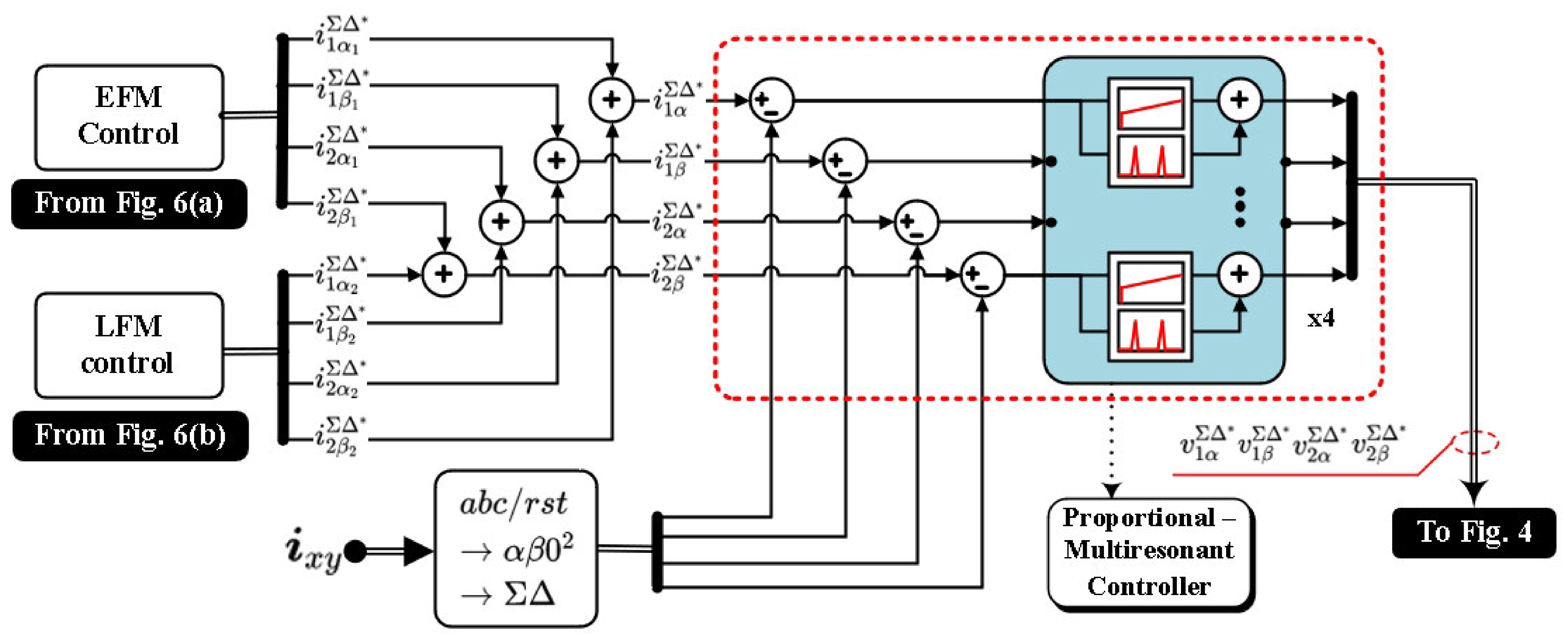
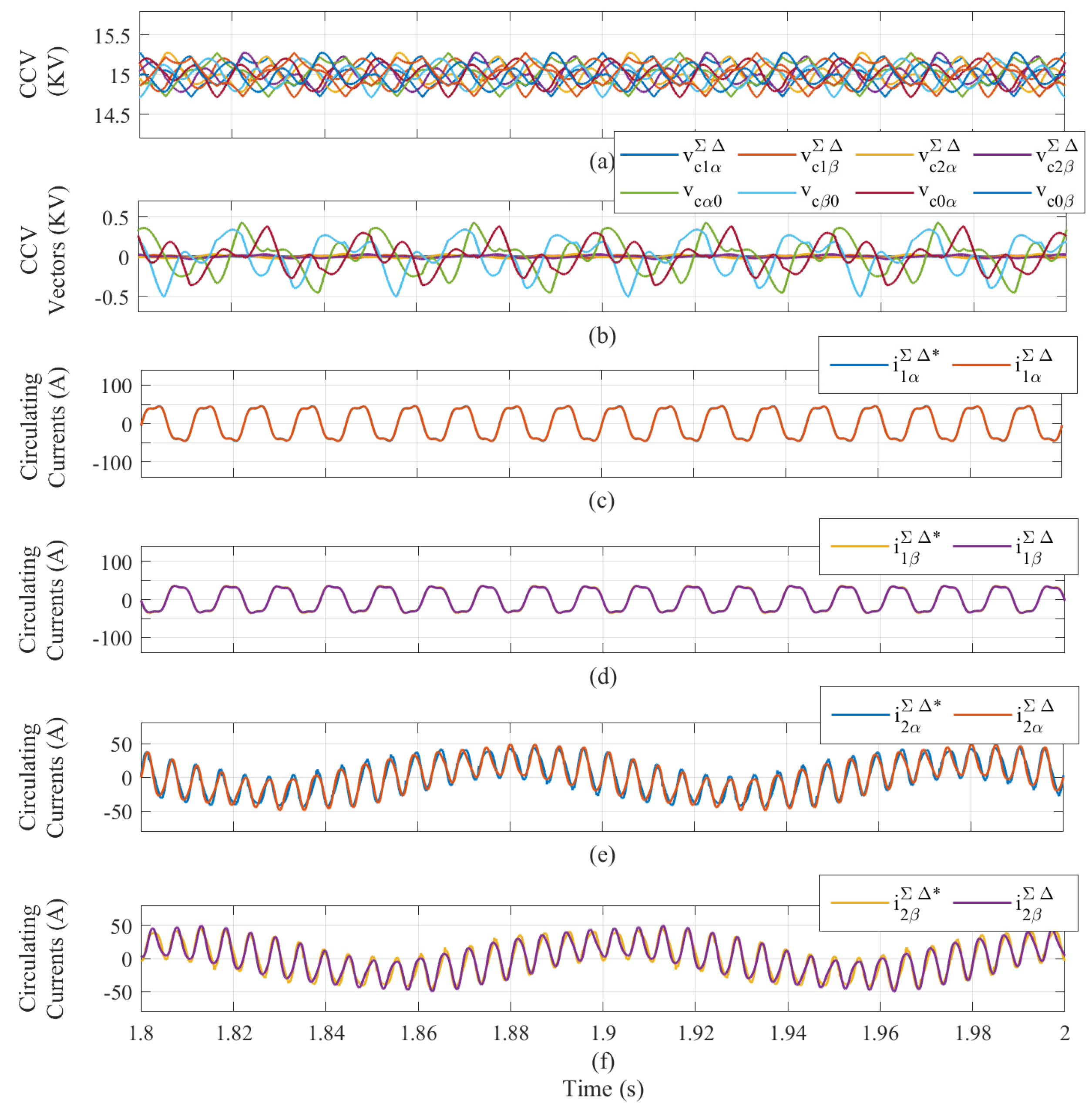
• The circulating current control is enhanced using proportional-resonant controllers implemented in the synchronous frame. This is different from the control systems previously published for $M^{3}C$ applications (see [15,16,17,18,23,26]) where proportional controllers implemented in the stationary $\alpha \beta$ frame were utilized, which cannot ensure zero steady-state error.

The rest of this paper is structured as follows: The modeling and control of the $M^{3}C$ are described in Section 2, Section 3, and Section 4. Vector control systems are used to regulate the floating capacitor voltages as proposed in [19,20]. Simulation results considering a 10 MW model are included to validate the effectiveness of the proposed control strategies. Finally, partial experimental results conducted with a 27-cell 5 kVA prototype are included.

2. Analysis of the ${\mathit{M}}^{\mathbf{3}}\mathit{C}$

The double $\alpha \beta 0$ transformation has been proposed to obtain a decoupled analysis and control of the $M^{3}C$ [22]. An additional transformation, referred to as $\Sigma \Delta$ transformation, can be applied to obtain a better representation of the circulating currents [23]. Additionally, the vector representation, proposed in [19,20], can be used to apply vector control strategies to regulate the floating capacitor voltages. In this work, the $M^{3}C$ dynamic model of the $M^{3}C$ is expressed in vector notation using the double $\alpha \beta 0$-$\Sigma \Delta$ frame.

2.1. Voltage-Current Model of the $M^{3}C$

Using the Kirchhoff voltage law over the topology of the $M^{3}C$ presented in Figure 1b, the voltages and current across the converter can be related as follows:

$$\begin{array}{cc}\hfill \left[\begin{array}{ccc}{v}_{i_a}& v_{i_b}& v_{i_c}\\ v_{i_a}& v_{i_b}& v_{i_c}\\ v_{i_a}& v_{i_b}& v_{i_c}\end{array}\right]=L_c\frac{d}{dt}\left[\begin{array}{ccc}{i}_{ar}& i_{br}& i_{cr}\\ i_{as}& i_{bs}& i_{cs}\\ i_{at}& i_{bt}& i_{ct}\end{array}\right]+\left[\begin{array}{ccc}{v}_{ar}& v_{br}& v_{cr}\\ v_{as}& v_{bs}& v_{cs}\\ v_{at}& v_{bt}& v_{ct}\end{array}\right]& +\left[\begin{array}{ccc}{v}_{o_r}& v_{o_r}& v_{o_r}\\ v_{o_s}& v_{o_s}& v_{o_s}\\ v_{o_t}& v_{o_t}& v_{o_t}\end{array}\right]+v_n\left[\begin{array}{ccc}1& 1& 1\\ 1& 1& 1\\ 1& 1& 1\end{array}\right]\hfill \end{array}$$

(1)

where the input voltages are denoted by $v_{i_x}$, with $x\in a,b,c$, the output voltages are denoted by $v_{o_x}$, with $x\in r,s,t$, $i_{x}y$ stands for the cluster currents, $v_{x}y$ represents the output cluster voltages, $L_c$ stands for the cluster inductance, and $v_n$ is the common-mode voltage.

The $\Sigma \Delta$ double-$\alpha \beta 0$ transformation is applied to (1), yielding:

$$\begin{array}{cc}\hfill \sqrt{3}\left[\begin{array}{ccc}0& 0& 0\\ 0& 0& 0\\ v_{i_{\alpha }}& v_{i_{\beta }}& v_{i_0}\end{array}\right]=L_c\frac{d}{dt}\left[\begin{array}{ccc}{i}_{\alpha \alpha }^{\Sigma \Delta }& i_{\beta \alpha }^{\Sigma \Delta }& i_{0\alpha }\\ i_{\alpha \beta }^{\Sigma \Delta }& i_{\beta \beta }^{\Sigma \Delta }& i_{0\beta }\\ i_{\alpha 0}& i_{\beta 0}& i_{00}\end{array}\right]& +\left[\begin{array}{ccc}{v}_{\alpha \alpha }& v_{\beta \alpha }& v_{0\alpha }\\ v_{\alpha \beta }& v_{\beta \beta }& v_{0\beta }\\ v_{\alpha 0}& v_{\beta 0}& v_{00}\end{array}\right]+\sqrt{3}\left[\begin{array}{ccc}0& 0& v_{o_{\alpha }}\\ 0& 0& v_{o_{\beta }}\\ 0& 0& v_{o_0}\end{array}\right]+\left[\begin{array}{ccc}0& 0& 0\\ 0& 0& 0\\ 0& 0& 3v_n\end{array}\right]\hfill \end{array}$$

(2)

From the voltage-current model of the $M^{3}C$ presented in (2), it can be deduced that the input port can be regulated using the currents $i_{0\alpha }$ and $i_{0\beta }$, whereas the output port can be regulated using $i_{\alpha 0}$ and $i_{\beta 0}$. Additionally, the circulating currents $i_{\alpha \alpha }^{\Sigma \Delta }$, $i_{\beta \alpha }^{\Sigma \Delta }$, $i_{\beta \alpha }^{\Sigma \Delta }$, and $i_{\beta \beta }^{\Sigma \Delta }$ can be used to regulate the floating capacitor voltages as they are totally independent of the other systems.

2.2. Power-CCV Model of the $M^{3}C$

The total capacitor voltage available within a cluster, i.e., $v_{c_{xy}}={\sum }_{i=1}^n{v}_{c_{xyi}}$ ($x\in \{a,b,c\}$ and $y\in \{r,s,t\}$), is referred to as Cluster Capacitor Voltage (CCV). Assuming that all the power cells have the same capacitance C, dismissing internal looses, and considering that the capacitor voltages are well regulated to the demanded voltage $v_c^{*}$, the CCVs can be related to the cluster power as follows:

$$\begin{array}{c}\hfill C{v}_c^{*}\frac{d}{dt}\left[\begin{array}{ccc}{v}_{c_{ar}}& v_{c_{as}}& v_{c_{at}}\\ v_{c_{br}}& v_{c_{bs}}& v_{c_{bt}}\\ v_{c_{cr}}& v_{c_{cs}}& v_{c_{ct}}\end{array}\right]\approx \left[\begin{array}{ccc}{P}_{ar}& P_{as}& P_{at}\\ P_{br}& P_{bs}& P_{bt}\\ P_{cr}& P_{cs}& P_{ct}\end{array}\right]\end{array}$$

(3)

where the cluster power is calculated as $P_{xy}=v_{xy}{i}_{xy}$. Notice that in (3), the voltages $v_{C_{xy}}$ have small variations around the dc-value $v_c^{*}$.

As mentioned before, the CCVs can fluctuate during the operation of the converter, and complex control strategies are required at some input-output frequencies. The fluctuations of the CCVs with those conditions are presented in Figure 2. Notice that in this graphic, $V_{c_{ar}}$ stands for the fluctuations of the voltages, and the dc value of ≈$v_C^{*}$ has not been considered in $V_{c_{ar}}$. Additionally, unit power factor operation at the input is used to obtain Figure 2.

Using simulation, the parameters of Section 5 are used to plot the CCV oscillations as a function of the input-output port ratio and power factor. From Figure 2, it is concluded that larger CCV oscillations are generated when $f_i=\pm f_o$ and the Power Factor (PF) in the output port is near zero.

Applying the double $\alpha \beta 0-\Sigma \Delta$ transformation, the CCVs can be presented as follows:

$$\begin{array}{c}\hfill C{v}_c^{*}\frac{d}{dt}\left[\begin{array}{ccc}{v}_{c_{1\alpha }}^{\Sigma \Delta }& v_{c_{1\beta }}^{\Sigma \Delta }& v_{c_{0\alpha }}\\ v_{c_{2\alpha }}^{\Sigma \Delta }& v_{c_{2\beta }}^{\Sigma \Delta }& v_{c_{0\beta }}\\ v_{c_{\alpha 0}}& v_{c_{\beta 0}}& v_{c_{00}}\end{array}\right]\approx \left[\begin{array}{ccc}{P}_{1\alpha }^{\Sigma \Delta }& P_{1\beta }^{\Sigma \Delta }& P_{0\alpha }\\ P_{2\alpha }^{\Sigma \Delta }& P_{2\beta }^{\Sigma \Delta }& P_{0\beta }\\ P_{\alpha 0}& P_{\beta 0}& P_{00}\end{array}\right]\end{array}$$

(4)

The terms $v_{c_{1\alpha }}^{\Sigma \Delta }$, $v_{c_{1\beta }}^{\Sigma \Delta }$, $v_{c_{2\alpha }}^{\Sigma \Delta }$, $v_{c_{2\beta }}^{\Sigma \Delta }$, $v_{c_{0\alpha }}$, $v_{c_{0\beta }}$, $v_{c_{\alpha 0}}$, and $v_{c_{\beta 0}}$ represent CCV imbalances, and they should tend to zero if the $M^{3}C$ is properly regulated. Additionally, $v_{c_{00}}$ is related to the total active power flowing into/from the $M^{3}C$ and can be regulated to set the total average value of the CCVs.

The CCV-power model can be expressed as a function of the circulating currents and the common-mode voltage [19,20]:

$$\begin{array}{c}\hfill C{v}_c^{*}\frac{d{\mathit{v}}_{c_1\alpha \beta }^{\Sigma \Delta }}{dt}\approx {\mathit{P}}_{1\alpha \beta }^{\Sigma \Delta }=\frac{1}{6}\left({\mathit{v}}_{i_{\alpha \beta }}^c{\mathit{i}}_{o_{\alpha \beta }}-{\mathit{v}}_{o_{\alpha \beta }}{\mathit{i}}_{i_{\alpha \beta }}^c\right)+\frac{1}{\sqrt{6}}\left({\mathit{v}}_{i_{\alpha \beta }}{\mathit{i}}_{2\alpha \beta }^{\Sigma \Delta }-{\mathit{v}}_{o_{\alpha \beta }}^c{\mathit{i}}_{2\alpha \beta }^{\Sigma \Delta c}\right)-v_n{\mathit{i}}_{1\alpha \beta }^{\Sigma \Delta }\end{array}$$

(5)

$$\begin{array}{c}\hfill C{v}_c^{*}\frac{d{\mathit{v}}_{c_2\alpha \beta }^{\Sigma \Delta }}{dt}\approx {\mathit{P}}_{2\alpha \beta }^{\Sigma \Delta }=\frac{1}{6}\left({\mathit{v}}_{i_{\alpha \beta }}{\mathit{i}}_{o_{\alpha \beta }}-{\mathit{v}}_{o_{\alpha \beta }}{\mathit{i}}_{i\alpha \beta }\right)+\frac{1}{\sqrt{6}}\left({\mathit{v}}_{i_{\alpha \beta }}^c{\mathit{i}}_{1\alpha \beta }^{\Sigma \Delta }-{\mathit{v}}_{o_{\alpha \beta }}^c{\mathit{i}}_{1\alpha \beta }^{\Sigma {\Delta }^c}\right)-v_n{\mathit{i}}_{2\alpha \beta }^{\Sigma \Delta }\end{array}$$

(6)

$$\begin{array}{c}\hfill C{v}_c^{*}\frac{d{\mathit{v}}_{c_0}^{\alpha \beta }}{dt}\approx {\mathit{P}}_0^{\alpha \beta }=\frac{1}{3\sqrt{2}}\left({\mathit{v}}_{i_{\alpha \beta }}^c{\mathit{i}}_{i_{\alpha \beta }}^c\right)-\frac{1}{\sqrt{3}}\left({\mathit{v}}_{o_{\alpha \beta }}{\mathit{i}}_{1\alpha \beta }^{\Sigma {\Delta }^c}+{\mathit{v}}_{o_{\alpha \beta }}^c{\mathit{i}}_{2\alpha \beta }^{\Sigma \Delta }+v_n{\mathit{i}}_{i_{\alpha \beta }}\right)\end{array}$$

(7)

$$\begin{array}{c}\hfill C{v}_c^{*}\frac{d{\mathit{v}}_{c_{\alpha \beta }}^0}{dt}\approx {\mathit{P}}_{\alpha \beta }^0=\frac{-1}{3\sqrt{2}}\left({\mathit{v}}_{o_{\alpha \beta }}^c{\mathit{i}}_{o_{\alpha \beta }}^c\right)+\frac{1}{\sqrt{3}}\left({\mathit{v}}_{i_{\alpha \beta }}{\mathit{i}}_{1\alpha \beta }^{\Sigma \Delta }+{\mathit{v}}_{i_{\alpha \beta }}^c{\mathit{i}}_{2\alpha \beta }^{\Sigma \Delta }-v_n{\mathit{i}}_{o_{\alpha \beta }}\right)\end{array}$$

(8)

where the superscript c represents the complex conjugate operator, the variables ${\mathit{v}}_{i_{\alpha \beta }}$ and ${\mathit{i}}_{i_{\alpha \beta }}$ represent the input-port voltages and currents in the $\alpha \beta 0$ frame, and the variables ${\mathit{v}}_{o_{\alpha \beta }}$ and ${\mathit{i}}_{o_{\alpha \beta }}$ represent the output-port voltages and currents in the $\alpha \beta 0$ frame. The CCV vectors ${\mathit{v}}_{c_1\alpha \beta }^{\Sigma \Delta }$, ${\mathit{v}}_{c_2\alpha \beta }^{\Sigma \Delta }$, ${\mathit{v}}_{c_{\alpha \beta }}^0$, and ${\mathit{v}}_{c_0}^{\alpha \beta }$ are independently related to the input-output port frequency conditions as follows:

• ${\mathit{v}}_{c_1\alpha \beta }^{\Sigma \Delta }$ has a dominant frequency oscillation of $f_o-f_i$.
• ${\mathit{v}}_{c_2\alpha \beta }^{\Sigma \Delta }$ has a dominant frequency oscillation of $f_i+f_o$.
• ${\mathit{v}}_{c_0}^{\alpha \beta }$ has a dominant frequency oscillation of $2f_i$.
• ${\mathit{v}}_{c_{\alpha \beta }}^0$ has a dominant frequency oscillation of $2f_o$.

For UPFC applications, where the input port frequency $f_i$ is equal to the output port frequency $f_o$, large oscillations appear just in ${\mathit{v}}_{c_1\alpha \beta }^{\Sigma \Delta }$, and EFM control strategies must be applied.

3. Proposed Vector Control Strategy

The overview of the proposed vector control strategy for the $M^{3}C$ based UPFC applications is presented in Figure 3. The cascaded control structure enables decoupled input-output ports control, as well as decoupled regulation of the CCVs in the double $\alpha \beta 0-\Sigma \Delta$ frame.The $M^{3}C$ control systems are depicted in Figure 4. Notice that the acronym $LFM$ stands for low frequency operation.

3.1. Control of the Input-Output Ports

The input port control diagram is presented in Figure 5a. Similar to previous works, $v_{c_{00}}$ is used to regulate the average total value of the CCVs. This imposes a direct input port current reference $i_{d01}^{*}$, which is superposed on an active power current reference. Additionally, as the input port currents are regulated in a $dq$ frame, it is possible to regulate active and reactive power independently. It should be mentioned that the reactive power reference can be changed from a fixed set-point to a $\Delta Q$ calculated in order to fulfill shunt FACTS requirements (see Figure 8a).

On the other hand, the output port current control diagram is presented in Figure 5b. Similarly, the current references are calculated from the reactive and active power set-points and implemented in a synchronous $dq$ frame rotating at $f_o$. It is important to highlight that the control diagram of Figure 5b is modified as explained in Section 4 to enable the UPFC capabilities.

3.2. $M^{3}C$ Control

In this proposal, the $M^{3}C$ control is divided into CCV control, circulating current control, and single-cell control. An overview of the proposed control system is shown in Figure 4, and each sub-control system is described in the next subsections.

Besides regulating the average value of all the floating capacitor voltages using the component $v_{c_{00}}$, the CCVs, i.e., ${\mathit{v}}_{c_{1\alpha \beta }}^{\Sigma \Delta }$, ${\mathit{v}}_{c_{2\alpha \beta }}^{\Sigma \Delta }$,${\mathit{v}}_{c_0}^{\alpha \beta },{\mathit{v}}_{c_{\alpha \beta }}^0$, must be controlled to achieve proper floating capacitor voltage control of the $M^{3}C$.

3.2.1. CCV Control

As the UPFC application implies equal frequencies at the input-output ports, ${\mathit{v}}_{c_{1\alpha \beta }}^{\Sigma \Delta }$ is regulated using an EFM control strategy. Therefore, (5) is referred to a synchronous reference frame rotating at $f_{u_1}=f_o-f_i$ yielding:

$$\begin{array}{c}\hfill C{v}_c^{*}(\frac{d{\mathit{v}}_{c_{1_{d}q}}^{\Sigma \Delta }}{dt}+j2\pi f_{u_1}{\mathit{v}}_{c_{1dq}}^{\Sigma \Delta })\approx \frac{1}{6}({\mathit{v}}_{i_{dq}}^c{\mathit{i}}_{o_{dq}}-{\mathit{v}}_{o_{dq}}{\mathit{i}}_{i_{dq}}^c)+\frac{1}{\sqrt{6}}({\mathit{v}}_{i_{dq}}{\mathit{i}}_{2dq}^{\Sigma \Delta }{e}^{j{3\theta }_i}-{\mathit{v}}_{g_{dq}}^c{\mathit{i}}_{2dq}^{\Sigma \Delta c}{e}^{-j3{\theta }_o})-v_n{\mathit{i}}_{1dq}^{\Sigma \Delta }\end{array}$$

(9)

Neglecting high-frequency terms, (9) becomes:

$$\begin{array}{c}\hfill C{v}_c^{*}\frac{d{\mathit{v}}_{c_{1dq}}^{\Sigma \Delta }}{dt}\approx \frac{1}{6}({\mathit{v}}_{i_{dq}}^c{\mathit{i}}_{o_{dq}}-{\mathit{v}}_{o_{dq}}{\mathit{i}}_{i_{dq}}^c)-V_{00}{\mathit{i}}_{1d{q}_1}^{\Sigma \Delta }\end{array}$$

(10)

The first term of the right side of (11) can be fed-forward to the total circulating current. Then, (11) yields:

$$\begin{array}{c}\hfill C{v}_c^{*}\frac{d{\mathit{v}}_{c_{1dq}}^{\Sigma \Delta }}{dt}\approx -V_{00}{\mathit{i}}_{1d{q}_1}^{\Sigma \Delta }\end{array}$$

(11)

The first term of the right side of (11), i.e., a product of circulating currents and common mode voltage, is used to mitigate the oscillations in ${\mathit{v}}_{c_{1\alpha \beta }}^{\Sigma \Delta }$ in a $dq$ rotating frame as shown in Figure 6a. The common-mode voltage and the $dq$ circulating currents should be in phase to efficiently produce adjustable power flow to drive the CCVs to zero. These variables are defined as follows:

$$\begin{array}{c}\hfill {\mathit{i}}_{1d{q}_1}^{\Sigma \Delta *}={\mathit{I}}_{1d{q}_1}^{\Sigma \Delta *}f\left(t\right);{\mathit{i}}_{2d{q}_1}^{\Sigma \Delta *}={\mathit{I}}_{2d{q}_1}^{\Sigma \Delta *}f\left(t\right);v_n=V_{00}g\left(t\right)\end{array}$$

(12)

where $f\left(t\right)$ is defined as $f\left(t\right)=A_{1}sin{\theta }_n+A_{3}sin{3\theta }_n$, with the angle ${\theta }_n$ set at a relatively high frequency. The function $g\left(t\right)$ is defined as $g\left(t\right)=\mathrm{sign}\left\{f\right(t\left)\right\}$. The amplitudes of the constants $A_1$, $A_3$, and $V_0$ are chosen to reduce the peak of the circulating currents as proposed in [29]. More details about the selection of the circulating currents and common-mode voltage were detailed in [20]. Additionally, an analysis of the magnitude and frequency of the common-mode voltage was presented in [29].

In the case of the remaining CCV vectors, DFM control is applied as shown in Figure 6. As the oscillations in ${\mathit{v}}_{c_{2\alpha \beta }}^{\Sigma \Delta }$, ${\mathit{v}}_{c_0}^{\alpha \beta }$, and ${\mathit{v}}_{c_{\alpha \beta }}^0$ have frequencies of $f_i+f_o$, $2f_i$, and $2f_o$, respectively, it is assumed that the capacitance of each power cells is sufficient to attenuate the frequency oscillations, and only the average value of the CCVs is regulated. Then, the CCVs are filtered to obtain their average values, and (6)–(8) yield:

$$\begin{array}{c}\hfill C{v}_c^{*}\frac{d}{dt}{\overline{\mathit{v}}}_{c_{2\alpha \beta }}^{\Sigma \Delta }\approx -v_n{\mathit{i}}_{2d{q}_1}^{\Sigma \Delta }\\ \hfill C{v}_c^{*}\frac{d}{dt}{\overline{\mathit{v}}}_{c_0}^{\alpha \beta }\approx -\frac{{\mathit{v}}_{o_{dq}}{\mathit{i}}_{1d{q}_2}^{\Sigma \Delta c}}{\sqrt{3}}\\ \hfill C{v}_c^{*}\frac{d}{dt}{\overline{\mathit{v}}}_{c_{\alpha \beta }}^0\approx -\frac{{\mathit{v}}_{i_{dq}}^c{\mathit{i}}_{2d{q}_2}^{\Sigma \Delta }}{\sqrt{3}}\end{array}$$

(13)

The average value of the vector ${\mathit{v}}_{c_{2\alpha \beta }}^{\Sigma \Delta }$ is regulated using circulating currents and common-mode voltage, as presented in Figure 6a. On the other hand, vectors ${\mathit{v}}_{c_0}^{\alpha \beta }$ and ${\mathit{v}}_{c_{\alpha \beta }}^0$ are regulated using circulating currents in phase with the input and output voltages as presented in Figure 6b.

From (13), it is straightforward to identify the circulating current components required to regulate the average value of the CCVs, which are obtained from the control diagram presented in Figure 6.

3.2.2. Circulating Current Control

The output of the EFM and DFM control systems set the references of the circulating current control. As there are four CCV vectors and just two circulating current vectors, superposition of the references from the EFM and DFM control system is used:

$$\begin{array}{c}\hfill {\mathit{i}}_{1\alpha \beta }^{\Sigma \Delta *}={\mathit{i}}_{1\alpha {\beta }_1}^{\Sigma \Delta *}+{\mathit{i}}_{1\alpha {\beta }_2}^{\Sigma \Delta *}\\ \hfill {\mathit{i}}_{2\alpha \beta }^{\Sigma \Delta *}={\mathit{i}}_{2\alpha {\beta }_1}^{\Sigma \Delta *}+{\mathit{i}}_{2\alpha {\beta }_2}^{\Sigma \Delta *}\end{array}$$

(14)

The proposed circulating current control system is shown in Figure 7. The circulating currents are referred to the $\Sigma \Delta$ double-$\alpha \beta 0$ frame to be regulated by the proposed controller. Each circulating current is controlled using Proportional Multi-Resonant (PMR) controllers, which are tuned to regulate the circulating current harmonics produced by the CCV control systems. This is certainly an improvement over the conventional control approach where proportional controllers are used [15,16,17,18,23,26].

The output of the control system shown in Figure 7 is the cluster voltage references in the $\Sigma \Delta$ double-$\alpha \beta 0$ frame, i.e., ${\mathit{v}}_{1\alpha \beta }^{\Sigma \Delta *}$, ${\mathit{v}}_{2\alpha \beta }^{\Sigma \Delta *}$, ${\mathit{v}}_0^{\alpha \beta *},{\mathit{v}}_{\alpha \beta }^{0*}$. These voltage references are referred back to the $abc$-$rst$ frame to be processed by the single-cell control.

3.2.3. Single-Cell Control

The cluster voltage references are referred back to the $abc$-$rst$ frame using the inverse $\Sigma \Delta$ double-$\alpha \beta 0$ transformation. At this point, one cluster voltage reference is obtained for each cluster $v_{xy}^{*}$, where $xϵ\{a,b,c\}$ and $yϵ\{r,s,t\}$. Finally, these voltages are controlled by the single-cell control to obtain the voltage reference for each cell as proposed in [7].

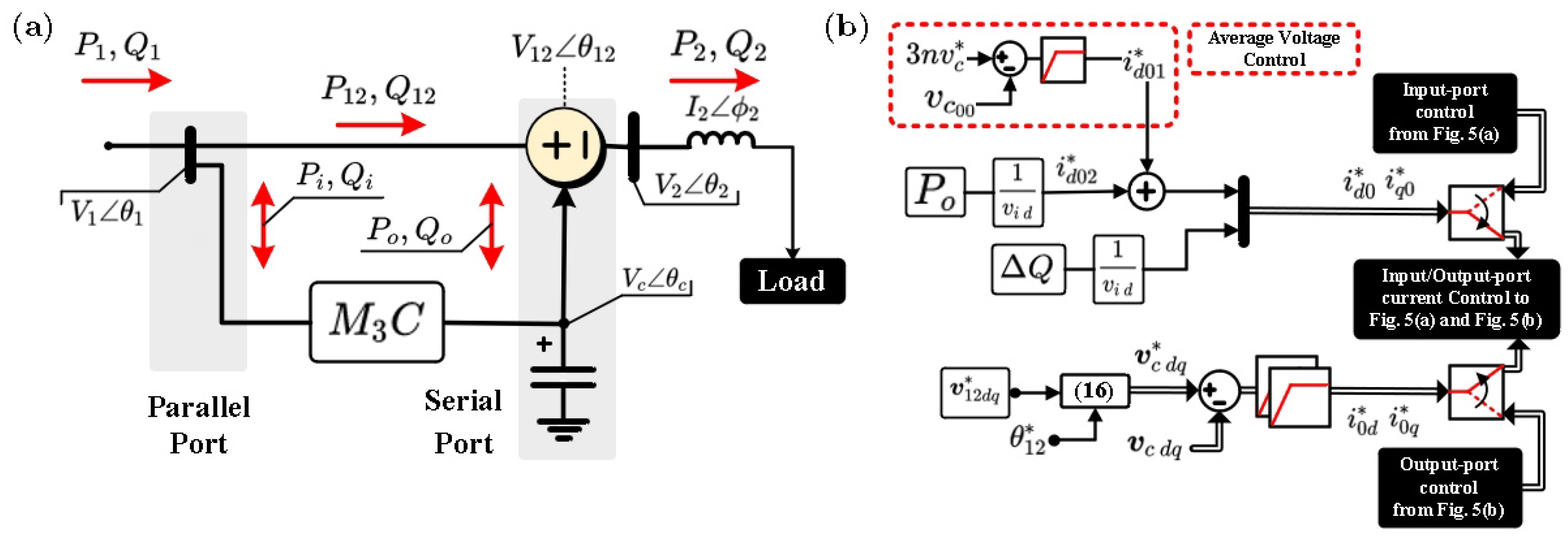
4. UPFC Control System

The $M^{3}C$ based UPFC topology is shown in Figure 8a. The input port of the $M^{3}C$ is connected to bus 1 to provide shunt FACT capabilities, whereas, the output port is connected to bus 2, and it is controlled as a series FACTS. The control strategy used to enable UPFC capabilities in both ports is presented in Figure 8b, and it is based on [30,31,32,33,34]:

4.1. Shunt Control FACT

In this case, the input port uses a similar control strategy as the direct power control shown previously in Figure 5a, operating in grid-following mode and oriented along with the voltage of bus 1. In order to represent voltage variations in bus 1, droop control is implemented at the $M^{3}C$ input port. The voltage variations are imposed by the reactive power $\Delta Q$, which corresponds to the reactive power required at bus 1.

4.2. Series Control FACT

The $M^{3}C$ output port is regulated in grid-forming mode as shown in Figure 8b. The proposed control strategy allows the regulation of the voltage $v_{cap}$. The controlled voltage is injected in series to the grid using a transformer as shown in Figure 8a. For the sake of simplicity, the transformer relation is 1:1 and then ${\mathit{v}}_{cap}={\mathit{v}}_{12}$.

The proposed control system regulates the amplitude and phase of ${\mathit{v}}_{12}$ using a nested control structure implemented in the $dq$ frame. The output port voltage module is determined by the ratio among the transferred power and the bus 2 current:

$${\mathit{v}}_{12}^{*}=k\frac{{\mathit{S}}_{12}^{*}}{{\mathit{i}}_2}$$

(15)

where the constant k is dependent on the selected $\alpha \beta 0$ transformation. Additionally, the angle reference is given by the required power factor of the injected power:

$${\theta }_{12}^{*}={\varphi }_2+\Delta {\varphi }^{*}$$

(16)

It is important to mention that the $dq$ control is oriented with ${\theta }_1$. Then, the $dq$ references are calculated as follows:

$$\begin{array}{c}\hfill v_{12d}^{*}=V_{12}^{*}sin\left({\theta }_{12}^{*}\right)\\ \hfill v_{12q}^{*}=-V_{12}^{*}cos\left({\theta }_{12}^{*}\right)\end{array}$$

(17)

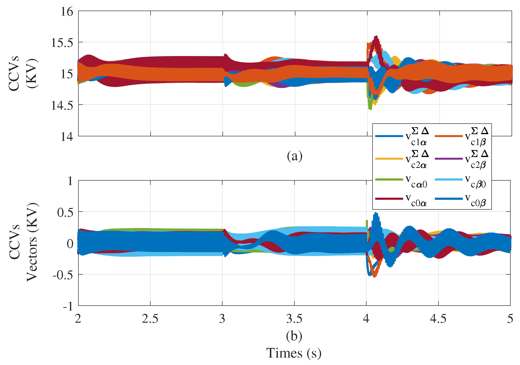
5. Simulation Results

Simulation results of a 10 MW $M^{3}C$ based UPFC were obtained to validate the feasibility of the theoretical work proposed in this paper. The model was developed in PLECS, and its main parameters are presented in

Table 1. Simulation parameters.

Simulation Parameter	Value
Nominal power	10 MW
Cells per branch	5
Input port voltage/frequency $f_i$	5.5 kV/50 Hz
Output port voltage/frequency $f_o$	5.39 kV/20–60 Hz
Cluster inductor $L_c$	1.3 $\mathrm{mH}$
Single-cell C	7000 uF
Single-cell capacitor voltage	3 kV
Common-mode voltage magnitude $V_{00}^{*}$	2 kV
UCC [35]	141.75 ms

.

The control strategies proposed in Figure 3, Figure 4, Figure 5 and Figure 6 were implemented using the model described in (5)–(8). The simulation results included three cases. The first test was carried out to verify the direct power control. The second test analyzed the behavior of the proposed CCV control with a focus on validating the proportional multi-resonant controller performance. Finally, the third test verified the operation of the $M^{3}C$ as UPFC.

In all the tests, $f_i=f_o$ and EFM was applied to ${\mathit{v}}_{c_{1\alpha \beta }}^{\Sigma \Delta }$, while DFM was applied to ${\mathit{v}}_{c_{2\alpha \beta }}^{\Sigma \Delta }$,${\mathit{v}}_{c_0}^{\alpha \beta }$, and ${\mathit{v}}_{c_{\alpha \beta }}^0$. The common-mode voltage had an amplitude of 2 $\mathrm{kV}$. Moreover, the common-mode voltage was defined as in Figure 5b with a frequency of $f_n=90$ Hz and third harmonic injection for the circulating currents [20].

Simulation results for the proposed direct power control are presented in Figure 9. The effectiveness of the control system was proven under different power conditions. In t = 2 s, the active power references decreased to 50% of the nominal value in both ports. At the same time, the reactive power of the input port $Q_i$ was set to $0.5MVA$, whereas the reactive power of the output port $Q_o$ was set to $-0.5MV{A}_r$. This operational point yielded large voltage oscillations, as shown in Figure 2, due to the $M^{3}C$ operating in EFM and the power factor of both ports was not unitary. Thereafter, in t = 4, the $M^{3}C$ operates with a unit power factor at both ports. During all the tests, the CCVs were properly regulated to their reference $v_c^{*}=15$ kV as shown in Figure 9a. Regardless of the complex operating point between t = 2 s and t = 4 s, the CCV vectors were successfully controlled as shown in Figure 9b, and the ripple was bounded inside a $\pm 500$ V band, which represented approximately <$5\%$ of the CCV reference voltage (15 kV). Additionally, Figure 9c verifies that the decoupled control of the power flows between ports was successfully obtained. The active and reactive powers tracked their references during the transition to opposite power factors (Intervals 2–4 seg).

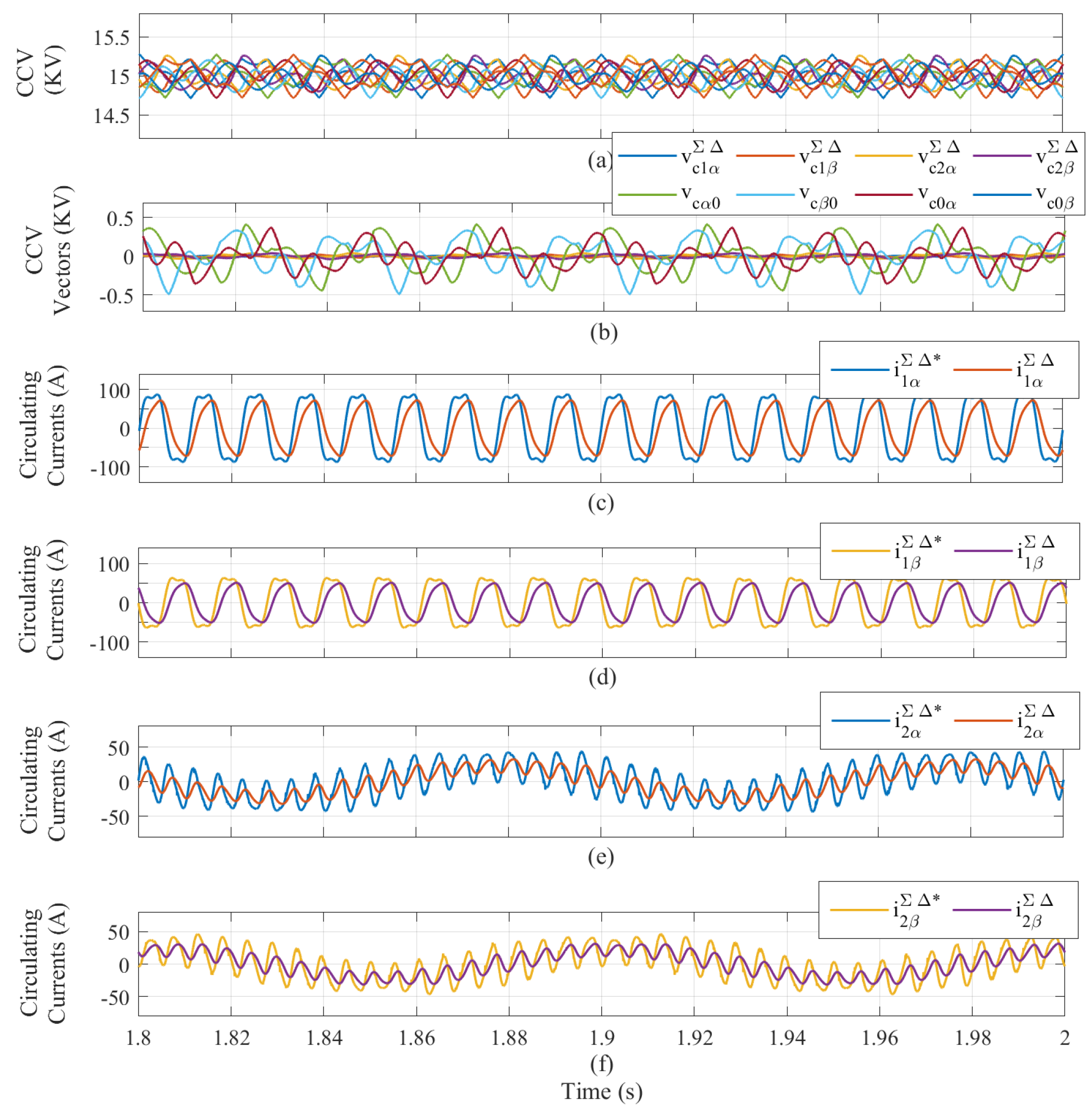
5.1. Test 2: Proportional Multi-Resonant Controller Performance

The results for the CCV vector control methodology (originally proposed in [20]), which utilises proportional controllers for the control of the circulating currents, are presented in Figure 10. Results for the proposed proportional multi-resonant circulating current control (see Figure 7) are presented in Figure 11. In order to address a fair comparison, in both cases, the $M^{3}C$ was operated with a unitary power factor and nominal power, and the common-mode voltage had an amplitude of 2 kV with a frequency of 90 Hz. Furthermore, there was a 20 ms time window to visualize the frequency components in the circulating currents.

As the EFM control of ${\mathit{v}}_{c_{1\alpha \beta }}^{\Sigma \Delta }$ and the DFM of ${\mathit{v}}_{c_{2\alpha \beta }}^{\Sigma \Delta }$ implied the injection of common-mode voltage, the multi-resonant controllers were tuned at $f_n$ Hz and $3f_n$ Hz to interact with the common-mode voltage and its third harmonic component. Moreover, the DFM control of ${\mathit{v}}_{c_0}^{\alpha \beta }$ and ${\mathit{v}}_{c_{\alpha \beta }}^0$ implied the interaction with the input-output port voltages (see Figure 6b and (13)), and then, the corresponding multi-resonant controllers were tuned also at $f_n\pm \left(f_i+f_o\right)$ Hz and $3f_n\pm \left(f_i+f_o\right)$.

The CCVs were successfully regulated to their nominal value of 15 kV as shown in Figure 10a and Figure 11a. Additionally, the regulation of CCV vectors (${\mathit{v}}_{c_{1\alpha \beta }}^{\Sigma \Delta }$, ${\mathit{v}}_{c_{2\alpha \beta }}^{\Sigma \Delta }$,${\mathit{v}}_{c_0}^{\alpha \beta }$, and ${\mathit{v}}_{c_{\alpha \beta }}^0$) was similar using both strategies, as shown in Figure 10b and Figure 11b.

Although both results presented comparable behavior, better regulation was obtained in circulating currents by using the method proposed in this paper. Comparing Figure 10c–f to Figure 11c–f, it was observed that zero steady-state error was possible when the proposed proportional multi-resonant control was used. What is more, the amplitude of ${\mathit{i}}_{1\alpha \beta }^{\Sigma \Delta }$ was reduced from 100 A (see Figure 10c,d) to 50 A (see Figure 11c,d). Considering that the cluster current of the $M^{3}C$ was composed of the sum of the input, output, and circulating currents, this reduction in ${\mathit{i}}_{1\alpha \beta }^{\Sigma \Delta }$ has a positive impact on cluster current stress.

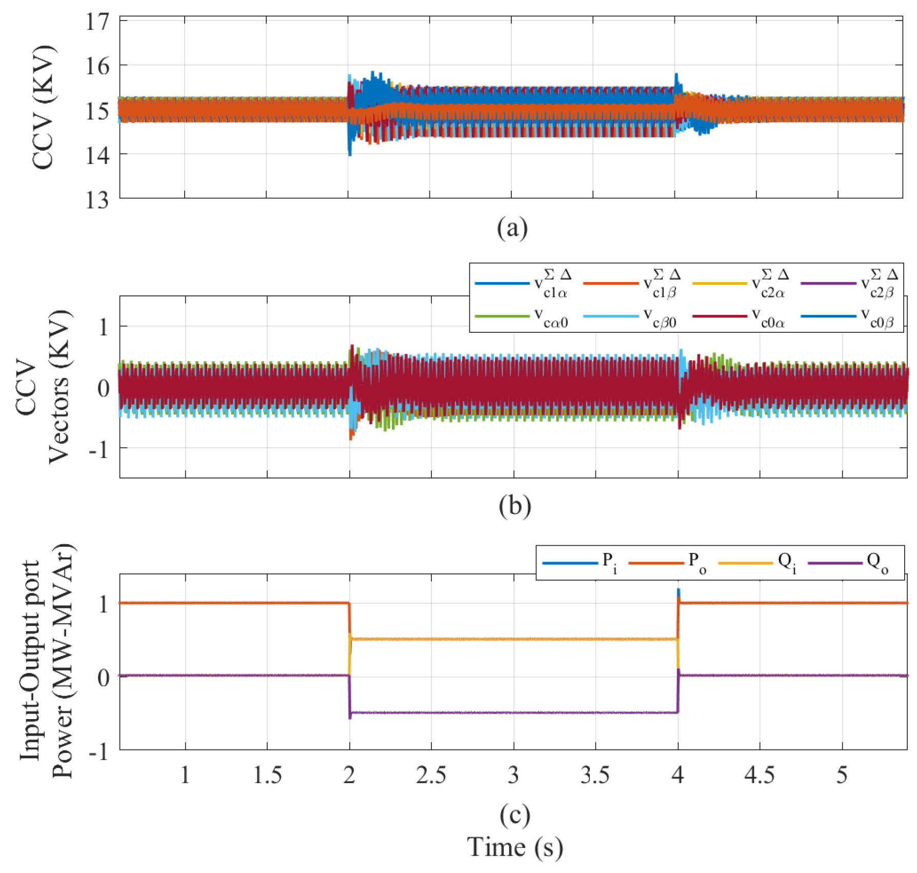
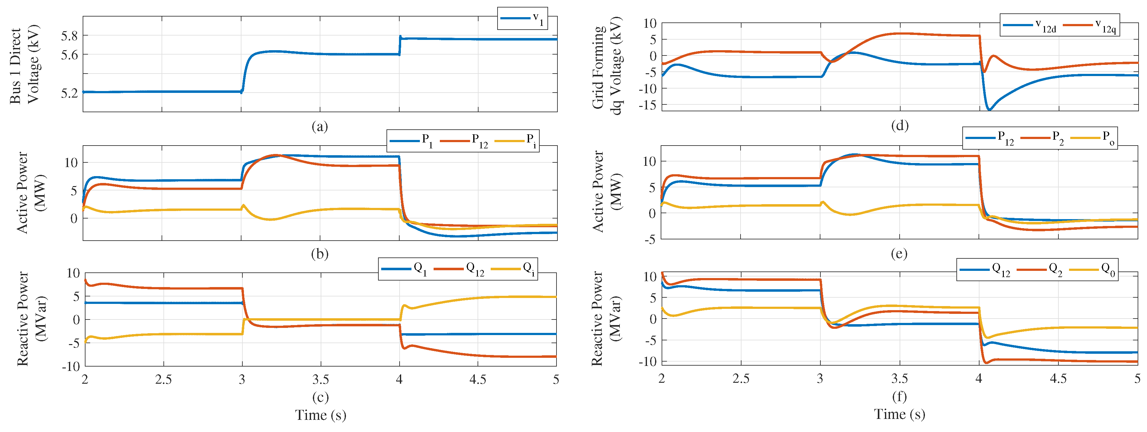
5.2. Test 3: UPFC Control

Results for a 10 MW $M^{3}C$ based UPFC are presented in Figure 12 and Figure 13. In this case, the input port was connected to bus 1 utilizing a shunt FACTS connection, whereas the output port was controlled as a series FACTS to manipulate $v_{12}$. The main variables of the shunt connection are shown in Figure 12a–c, and the main variables for the series connection are presented in Figure 12d,e. Additionally, the variables of the $M^{3}C$ are presented in Figure 13.

In Figure 12a, the direct voltage at bus 1 is presented. This voltage was controlled to not exceed a $\pm 5\%$ band. The active and reactive power components provided by the system ($P_1$, $Q_1$), transferred to bus 2 ($P_{12}$, $Q_{12}$), and compensated by the $M^{3}C$ ($P_i$ and $Q_i$) are presented in Figure 12b,c. Voltage control support was provided by the $M^{3}C$ through the injection of reactive power in the shunt port, as shown in Figure 12c.

The active and reactive powers at bus 1 are presented in Figure 12b,c. The power provided by the system ($P_1$, $Q_1$), the power transferred between bus 1 and bus 2 ($P_{12}$ and $Q_{12}$), and the power compensated by $M^{3}C$ ($P_i$ and $Q_i$) were regulated to provide voltage control support through the injection of reactive power. For instance, in t = 2, the load connected to bus 2 was inductive, and the $M^{3}C$ injected reactive power to bus 1 to keep the voltage bounded in a range of $\pm 5\%$. After that, the load became resistive, and the reactive power injected by the $M^{3}C$ was null. Finally, the load became capacitive, and the $M^{3}C$ consumed reactive power to keep the voltage in bus 1 inside the range mentioned above.

In Figure 12d, the direct and quadrature components of the series voltage $v_{12}$ are presented. This voltage was regulated using a grid-forming strategy. As presented in (15)–(16), a constant angle of ${30}^{\circ }$ was used. The total required power to bus 1 ($P_{12}$ and $Q_{12}$), the required power by the load and the line ($P_2$ and $Q_2$), and the series power injected by $M^{3}C$ ($P_o$ and $Q_o$) are presented in Figure 12e,f. In t = 2, the magnitude of the voltage $v_{12}$ was regulated at a fixed value of 5.5 kV, and its angle was adjusted to produce series compensation of the load consumption. Then, the $M^{3}C$ could inject or absorb active and reactive power at its output port, modifying the power flow in the line between bus 1 and bus 2.

Finally, the $M^{3}C$ main variables are presented in Figure 13, and the main $M^{3}C$ variables are shown. The CCVs are presented in Figure 13a, and the CCV vectors are presented in Figure 13b, exhibiting a correct steady-state performance in both cases.

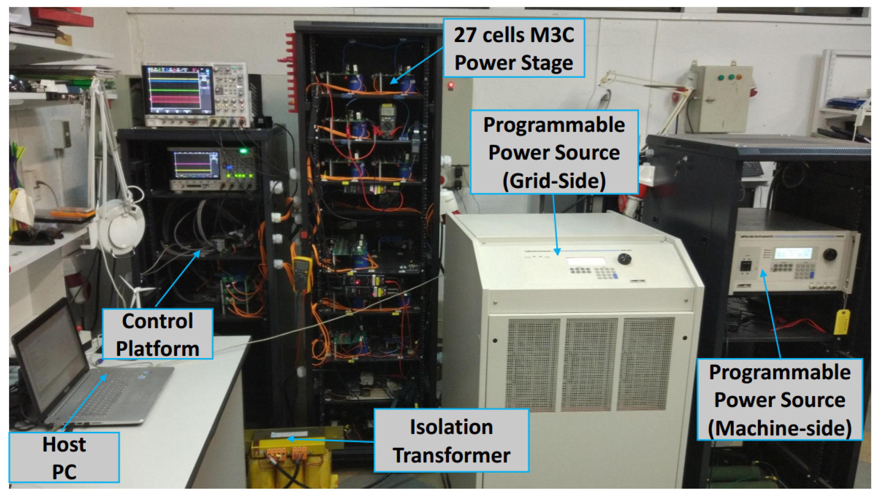
6. Experimental Results

In this section, experimental results for direct power control of an $M^{3}C$ based UPFC are presented. The experimental prototype is shown in Figure 14. The prototype was controlled using a Texas Instrument 6713C DSP board, equipped with three FPGA boards and additional external boards for computer communication and analogue-digital conversion. The power stage was composed of 27 full bridge power cells and nine 2.5 mH inductors. Each power cell was connected to a 4.7 mF floating capacitor. The output-port was connected to an Ametek Programmable power source, Model CSW5550, whereas the input-port was connected to a Ametek Programmable power source, model MX45.

Experimental results for the $M^{3}C$ prototype are presented in Figure 15. In this case, the direct power control strategy presented in Figure 5 was applied to regulate the input and output currents, whereas the $M^{3}C$ was operated using the control strategies described in Figure 3, Figure 4, Figure 6, and Figure 7.

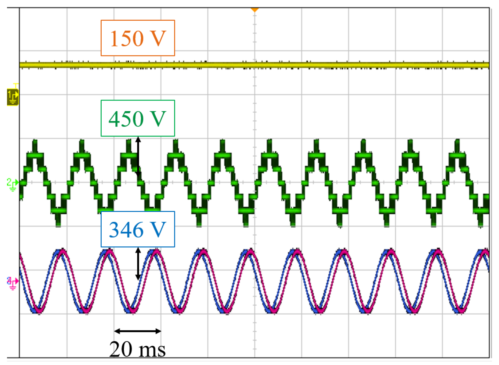
6.1. Test I: Steady-State Operation

The $M^{3}C$ operated with unity power factor injecting 3 kW to the output-port. The input/output port voltages were regulated to 200 V (peak value phase-to-neutral), and each capacitor was regulated at 150 V.

Scope waveforms of the voltages and currents of the $M^{3}C$ are presented in Figure 15. From top to bottom, the following variables are shown: one of the $M^{3}C$ capacitor voltages $v_{c_{ar1}}$; the cluster voltage $v_{ar}$; and the output and input voltages $v_{i_{ab}}$ (purple line) and $v_{o_{rt}}$ (blue line).

6.2. Test II: Direct Power Control

In this test, the active and reactive power components of both ports were independently controlled. Step changes in the active and reactive power were imposed during the test. The 27 capacitor voltages were well regulated to $v_c^{*}=150$ V regardless of the changes in the input-output powers, as shown in Figure 16a. Additionally, the input active power, input reactive power, output active power, and output reactive power are presented in Figure 16b.

7. Conclusions

A vector control strategy of an $M^{3}C$ based UPFC was proposed in this paper. The modeling and control of the converter were described and analyzed in the $\Sigma \Delta$ double-$\alpha \beta 0$ frame, permitting the implementation of cascaded vector control strategies. Moreover, the control of the $M^{3}C$ was improved by the introduction of proportional multi-resonant controllers that effectively regulated the circulating currents regardless of the frequency components and with zero steady-state error. The proposed control strategies regulated the input port in grid-feeding mode to provide shunt FACTS capabilities. At the same time, the output port was regulated in grid-forming mode to provide series FACTS compensation. Simulation results were presented to validate the effectiveness of the proposed control strategies. Results showed that the introduced multi-resonant circulating current controllers had adequate behavior and could reduce the circulating current requirement. Furthermore, the proposed control strategy for UPFC applications was verified for shunt and series FACTS control capabilities, while precise control of the $M^{3}C$ was achieved.

References

1. Kotsampopoulos, P.; Georgilakis, P.; Lagos, D.T.; Kleftakis, V.; Hatziargyriou, N. Facts providing grid services: Applications and testing. Energies 2019, 12, 2554. [Google Scholar] [CrossRef] [Green Version]
2. Hingorani, N.; Gyugyi, L. Understanding FACTS: Concepts and Technology of Flexible AC Transmission System, 1st ed.; Wiley-IEEE Press: New York, NY, USA, 2000. [Google Scholar]
3. Zhang, X.P.; Handschin, E.; Yao, M. Multi-control functional static synchronous compensator (STATCOM) in power system steady-state operations. Electr. Power Syst. Res. 2004, 72, 269–278. [Google Scholar] [CrossRef]
4. Sen, K.K. SSSC - Static Synchronous Series Compensator: Theory, modeling, and applications. IEEE Trans. Power Deliv. 1998, 13, 241–246. [Google Scholar] [CrossRef] [Green Version]
5. Li, M.; Lin, Z.; Wu, W.; Lin, Y.; Jiang, P.; Hu, Z.; Ye, R.; Du, Y. Application of UPFC in Fujian 500 kV power grid. J. Eng. 2019, 2019, 2510–2513. [Google Scholar] [CrossRef]
6. Kouro, S.; Rodriguez, J.; Wu, B.; Bernet, S.; Perez, M. Powering the future of industry: High-power adjustable speed drive topologies. IEEE Ind. Appl. Mag. 2012, 18, 26–39. [Google Scholar] [CrossRef]
7. Akagi, H. Classification, terminology, and application of the modular multilevel cascade converter (MMCC). IEEE Trans. Power Electron. 2011, 26, 3119–3130. [Google Scholar] [CrossRef]
8. Okazaki, Y.; Kawamura, W.; Hagiwara, M.; Akagi, H.; Ishida, T.; Tsukakoshi, M.; Nakamura, R. Experimental Comparisons Between Modular Multilevel DSCC Inverters and TSBC Converters for Medium-Voltage Motor Drives. IEEE Trans. Power Electron. 2017, 32, 1802–1817. [Google Scholar] [CrossRef]
9. Marquardt, R. Modular Multilevel Converter: An universal concept for HVDC-Networks and extended DC-bus-applications. In Proceedings of the 2010 International Power Electronics Conference—ECCE Asia, IPEC 2010, Sapporo, Japan, 21–24 June 2010; pp. 502–507. [Google Scholar] [CrossRef]
10. Allebrod, S.; Hamerski, R.; Marquardt, R. New transformerless, scalable modular multilevel converters for HVDC-transmission. In Proceedings of the PESC Record—IEEE Annual Power Electronics Specialists Conference, Rhodes, Greece, 15–19 June 2008; pp. 174–179. [Google Scholar] [CrossRef]
11. Zhuo, G.; Jiang, D.; Lian, X. Modular multilevel converter for unified power flow controller application. In Proceedings of the 2012 Third International Conference on Digital Manufacturing & Automation, GuiLin, China, 31 July–2 August 2012; pp. 545–549. [Google Scholar] [CrossRef]
12. Liu, J.; Xu, Z.; Xiao, L. Comprehensive power flow analyses and novel feedforward coordination control strategy for MMC-based UPFC. Energies 2019, 12, 824. [Google Scholar] [CrossRef] [Green Version]
13. Li, P.; Wang, Y.; Feng, C.; Lin, J. Application of MMC-UPFC in the 500 kV power grid of Suzhou. J. Eng. 2017, 2017, 2514–2518. [Google Scholar] [CrossRef]
14. Erickson, R.; Angkititrakul, S.; Almazeedi, K. A New Family of Multilevel Matrix Converters for Wind Power Applications: Final Report; National Renewable Energy Laboratory (NREL): Golden, CO, USA, 2006. [Google Scholar]
15. Díaz, M.; Cárdenas, R.; Mauricio Espinoza, B.; Mora, A.; Rojas, F. A novel LVRT control strategy for modular multilevel matrix converter based high-power wind energy conversion systems. In Proceedings of the 2015 10th International Conference on Ecological Vehicles and Renewable Energies, EVER 2015, Monte Carlo, Monaco, 31 March–2 April 2015; pp. 1–11. [Google Scholar] [CrossRef]
16. Diaz, M.; Rojas, F.; Donoso, F.; Cardenas, R.; Espinoza, M.; Mora, A.; Wheeler, P. Control of modular multilevel cascade converters for offshore wind energy generation and transmission. In Proceedings of the 2018 13th International Conference on Ecological Vehicles and Renewable Energies, EVER 2018, Monte-Carlo, Monaco, 10–12 April 2018; pp. 1–10. [Google Scholar] [CrossRef]
17. Diaz, M.; Cardenas, R.; Espinoza, M.; Rojas, F.; Mora, A.; Clare, J.C.; Wheeler, P. Control of Wind Energy Conversion Systems Based on the Modular Multilevel Matrix Converter. IEEE Trans. Ind. Electron. 2017, 64, 8799–8810. [Google Scholar] [CrossRef]
18. Fan, B.; Wang, K.; Wheeler, P.; Gu, C.; Li, Y. An Optimal Full Frequency Control Strategy for the Modular Multilevel Matrix Converter Based on Predictive Control. IEEE Trans. Power Electron. 2018, 33, 6608–6621. [Google Scholar] [CrossRef]
19. Diaz, M.; Espinosa, M.; Rojas, F.; Wheeler, P.; Cardenas, R. Vector control strategies to enable equal frequency operation of the modular multilevel matrix converter. J. Eng. 2019, 2019, 4214–4219. [Google Scholar] [CrossRef]
20. Diaz, M.; Cardenas, R.; Espinoza, M.; Hackl, C.M.; Rojas, F.; Clare, J.C.; Wheeler, P. Vector control of a modular multilevel matrix converter operating over the full output-frequency range. IEEE Trans. Ind. Electron. 2019, 66, 5102–5114. [Google Scholar] [CrossRef]
21. Kammerer, F.; Kolb, J.; Braun, M. Fully decoupled current control and energy balancing of the Modular Multilevel Matrix Converter. In Proceedings of the 2012 15th International Power Electronics and Motion Control Conference (EPE/PEMC), Novi Sad, Serbia, 4–6 September 2012; pp. LS2a.3:1–LS2a.3:8. [Google Scholar]
22. Kawamura, W.; Hagiwara, M.; Akagi, H. Experimental verification of a modular multilevel cascade converter based on triple-star bridge-cells (MMCC-TSBC) for motor drives. In Proceedings of the 2013 1st International Future Energy Electronics Conference (IFEEC), Tainan, Taiwan, 3–6 November 2014; Volume 50, pp. 454–459. [Google Scholar] [CrossRef]
23. Kammerer, F.; Gommeringer, M.; Kolb, J.; Braun, M. Energy balancing of the Modular Multilevel Matrix Converter based on a new transformed arm power analysis. In Proceedings of the 2014 16th European Conference on Power Electronics and Applications, EPE-ECCE Europe 2014, Lappeenranta, Finland, 26–28 August 2014. [Google Scholar] [CrossRef] [Green Version]
24. Xu, Q.; Ma, F.; Luo, A.; He, Z.; Xiao, H. Analysis and Control of M3C-Based UPQC for Power Quality Improvement in Medium/High-Voltage Power Grid. IEEE Trans. Power Electron. 2016, 31, 8182–8194. [Google Scholar] [CrossRef]
25. Monteiro, J.; Pinto, S.; Martin, A.D.; Silva, J.F. A new real time Lyapunov based controller for power quality improvement in Unified Power Flow Controllers using Direct Matrix Converters. Energies 2017, 10, 779. [Google Scholar] [CrossRef] [Green Version]
26. Kawamura, W.; Hagiwara, M.; Akagi, H. A broad range of frequency control for the modular multilevel cascade converter based on triple-star bridge-cells (MMCC-TSBC). In Proceedings of the 2013 IEEE Energy Conversion Congress and Exposition, ECCE 2013, Denver, CO, USA, 15–19 September 2013; pp. 4014–4021. [Google Scholar] [CrossRef]
27. Cárdenas, R.; Peña, R. Sensorless vector control of induction machines for variable-speed wind energy applications. IEEE Trans. Energy Convers. 2004, 19, 196–205. [Google Scholar] [CrossRef]
28. Espinoza, M.; Cárdenas, R.; Díaz, M.; Clare, J.C. An Enhanced dq-Based Vector Control System for Modular Multilevel Converters Feeding Variable-Speed Drives. IEEE Trans. Ind. Electron. 2017, 64, 2620–2630. [Google Scholar] [CrossRef]
29. Espinoza, M.; Espina, E.; Diaz, M.; Mora, A.; Cardenas, R. Improved control strategy of the modular multilevel converter for high power drive applications in low frequency operation. In Proceedings of the 2016 18th European Conference on Power Electronics and Applications (EPE’16 ECCE Europe), Karlsruhe, Germany, 5–9 September 2016; pp. 1–10. [Google Scholar] [CrossRef]
30. Fujita, H.; Watanabe, Y.; Akagi, H. Control and analysis of a unified power flow controller. IEEE Annu. Power Electron. 1998, 1, 805–811. [Google Scholar] [CrossRef] [Green Version]
31. Rem, B.A.; Keri, A.; Mehraban, A.S.; Schauder, C.; Stacey, E.; Kovalsky, L.; Gyugyi, L. Aep unified power flow controller performance. IEEE Trans. Power Deliv. 1999, 14, 1374–1381. [Google Scholar]
32. Zhu, P.; Liu, L.; Liu, X.; Kang, Y.; Chen, J.; Member, S. Analysis and Comparison of two Control Strategies for UPFC. In Proceedings of the 2005 IEEE/PES Transmission & Distribution Conference & Exposition: Asia and Pacific, Dalian, China, 18 August 2005; pp. 1–7. [Google Scholar]
33. Chen, J.; Tao, J.; Wang, C.; Wei, P.; Liu, J.; Li, Q.; Zhou, Q. Control strategy of UPFC based on power transfer distribution factor. J. Eng. 2019, 2019, 1897–1899. [Google Scholar] [CrossRef]
34. Zhang, J.; Hu, Z.; Cui, D.; Zhang, H. Research of MMC-UPFC Control Strategy. In Proceedings of the 2019 IEEE PES Innovative Smart Grid Technologies Asia, ISGT 2019, Chengdu, China, 21–24 May 2019; pp. 2217–2222. [Google Scholar] [CrossRef]
35. Fujita, H.; Tominaga, S.; Akagi, H. Analysis and design of a DC voltage-controlled static var compensator using quad-series voltage-source inverters. IEEE Trans. Ind. Appl. 1996, 32, 970–978. [Google Scholar] [CrossRef] [Green Version]
Figure 1. (a) Proposed Modular Multilevel Matrix Converter ( M 3 C )-Unified Power Flow Controller (UPFC) topology. (b) M 3 C topology. (c) Cluster composition.
Energies 13 00953 g001
Figure 2. Cluster Capacitor Voltage (CCV) (pu) vs. P F o vs. f o (pu).
Energies 13 00953 g002
Figure 3. Overview of the control system of the M 3 C topology in Equal Frequencies Mode (EFM).
Energies 13 00953 g003
Figure 4. Control system for the M 3 C .
Energies 13 00953 g004
Figure 5. (a) Input port power control. (b) Output port power control.
Energies 13 00953 g005
Figure 6. (a) EFM control strategy of v c 1 α β Σ Δ and Different Frequencies Mode (DFM) of v c 2 α β Σ Δ . (b) DFM control strategy of v c 0 α β and v c α β 0 .
Energies 13 00953 g006
Figure 7. Proposed proportional resonant control system for the circulating currents.
Energies 13 00953 g007
Figure 8. (a) Detailed proposed M 3 C -UPFC topology. (b) Proposed M 3 C -UPFC control system.
Energies 13 00953 g008
Figure 9. Test 1 results. (a) CCVs. (b) CCV vectors in the Σ Δ double- α β 0 frame. (c) Active and reactive power at the M 3 C input and output ports.
Energies 13 00953 g009
Figure 10. Test 1 results using proportional controllers. (a) CCVs. (b) CCV vectors in the Σ Δ double- α β 0 frame. (cf) Circulating current components in the Σ Δ double- α β 0 frame.
Energies 13 00953 g010
Figure 11. Test 2 results using a multi-resonant controller. (a) CCVs. (b) CCV vectors in the Σ Δ double- α β 0 frame. (cf) Circulating current components in the Σ Δ double- α β 0 frame.
Energies 13 00953 g011
Figure 12. (a) Direct voltage at bus 1. (b) Active power flows in the shunt port. (c) Reactive power flows in the shunt port. (d) v 12 direct and quadrature components. (e) Active power flows in the series port. (f) Reactive power flows in shunt port.
Energies 13 00953 g012
Figure 13. M 3 C operating as UPFC: (a) CCVs. (b) CCV vectors in the Σ Δ double- α β 0 frame.
Energies 13 00953 g013
Figure 14. M 3 C Laboratory prototype.
Energies 13 00953 g014
Figure 15. Experimental results.
Energies 13 00953 g015
Figure 16. Experimental results for changes in the input-output power components.
Energies 13 00953 g016