Article

Analysis of CO2 Drivers and Emissions Forecast in a Typical Industry-Oriented County: Changxing County, China

1
Key Laboratory of Urban Environment and Health, Institute of Urban Environment, Chinese Academy of Sciences, Xiamen 361021, China
2
University of Chinese Academy of Sciences, Beijing 100049, China
3
State Key Laboratory of Urban and Regional Ecology, Research Center for Eco-Environmental Sciences, Chinese Academy of Sciences, Beijing 100049, China
4
College of Geography and Environment, Shandong Normal University, Jinan 250014, China
*
Author to whom correspondence should be addressed.
Energies 2020, 13(5), 1212; https://doi.org/10.3390/en13051212
Submission received: 12 February 2020 / Revised: 2 March 2020 / Accepted: 4 March 2020 / Published: 6 March 2020
(This article belongs to the Section B: Energy and Environment)

Abstract

:
Decomposing main drivers of CO2 emissions and predicting the trend of it are the key to promoting low-carbon development for coping with climate change based on controlling GHG emissions. Here, we decomposed six drivers of CO2 emissions in Changxing County using the Logarithmic Mean Divisia Index (LMDI) method. We then constructed a model for CO2 emissions prediction based on a revised version of the Stochastic Impacts by Regression on Population, Affluence, and Technology (STIRPAT) model and used it to simulate energy-related CO2 emissions in five scenarios. Results show that: (1) From 2010 to 2017, the economic output effect was a significant, direct, dominant, and long-term driver of increasing CO2 emissions; (2) The STIRPAT model predicted that energy structure will be the decisive factor restricting total CO2 emissions from 2018 to 2035; (3) Low-carbon development in the electric power sector is the best strategy for Changxing to achieve low-carbon development. Under the tested scenarios, Changxing will likely reach peak total CO2 emissions (17.95 million tons) by 2030. Measures focused on optimizing the overall industrial structure, adjusting the internal industry sector, and optimizing the energy structure can help industry-oriented counties achieve targeted carbon reduction and control, while simultaneously achieving rapid economic development.

1. Introduction

Human health, ecosystems, and socio-economic systems are sensitive to the pace and extent of climate change, with some adverse impacts of climate change becoming persistent or irreversible. For example, global average surface warming by the end of the 21st century is projected to depend mainly on accumulative CO2 emissions. The massive emissions of CO2 from various human activities are key drivers of climate change issues such as global warming. For example, fossil fuel combustion is a major source of CO2 emissions [1,2]. Therefore, strategies that effectively control CO2 emissions and achieve low-carbon development are needed to mitigate climate change. The international community has largely reached a consensus on low-carbon development, with most countries participating in international agreements such as the United Nations Framework Convention on Climate Change (UNFCCC), the Kyoto Protocol, and the Copenhagen Accord. In order to achieve carbon emissions reduction targets, each contracting party shall formulate a low-carbon economic roadmap and strategic plan according to its individual circumstances, accelerate the development of low-carbon technologies, take initiative in the field of climate change mitigation, and pursue the support of international partners in these efforts in order to improve international competitiveness. In 2015, China submitted a report titled “Enhanced Actions on Climate Change: China’s Intended Nationally Determined Contributions” to the UNFCCC Secretariat, which set several national goals. In it, China committed to reaching peak CO2 emissions no later than 2030 and to decrease CO2 emissions per unit GDP by 60%–65% of 2005 levels. Subsequently, the Thirteenth Five-Year Plan for National Economic and Social Development of the People’s Republic of China (hereinafter referred to as the “13th Five-Year Plan”) states that “the total amount of carbon emissions needs to be effectively controlled” and “supports optimized development regions to achieve carbon emissions peak” [3].
The key to predicting total CO2 emissions is to scientifically extract the driving factors of CO2 emissions. Current research methods are mainly divided into two categories: econometrics and factor decomposition analysis. Econometric analysis has the advantage of flexibility but is prone to structural mutation problems for long-term sequence models [4]. Factor decomposition analysis can be divided into structural decomposition analysis (SDA), production theoretical decomposition analysis (PDA), and index decomposition analysis (IDA), according to different decomposition methods. The SDA is a static analysis method based on an input-output table, which is used to measure the contribution of each variable to the change in the dependent variable. However, due to the difficulty of obtaining input-output tables, the method is mostly used for the decomposition of carbon emissions at the national level [5,6]. As we know, the envelopment analysis method (DEA) has been successfully applied as models of analysis of eco-efficiency in global regions and countries [7]. Based on DEA, PDA proposed by Pasurka [8] is a data envelopment analysis model based on a distance function and the Malmquist Index. The advantage is that it can reflect the impact of the efficiency of various input/output factors on carbon emissions [9,10,11]. Compared with other methods, IDA’s biggest advantage is that data is relatively easy to obtain, the method is easy to use, and intuitive decomposition results are widely used at national, regional, and city scales [12,13,14,15,16,17]. The IDA mainly includes the following decomposition methods: Passche Index, Fisher Index, Marshall Edgeworth Index, Laspeyres Index, and Divisa Index [18]. Ang et al. [19] proposed the Logarithmic Mean Divisia Index (LMDI), which effectively solved the problem of residual and zero-value data processing in the exponential decomposition method. Xu and Ang [20] analyzed the development of IDA as applied in emission studies and concluded that LMDI has become an ideal decomposition method of IDA in the past few years.
Numerous research methods have been used to predict total CO2 emissions and CO2 trends, including the neural network model, global change integrated assessment model for China (IAMC), LEAP model, MARKAL-MACRO model, grey prediction model, gene expression programming model, IPAT model, and Stochastic Impacts by Regression on Population, Affluence, and Technology (STIRPAT) model, and others. Sangeetha and Amudha [21] used the BP neural network model based on particle swarm optimization to predict CO2 peaks at the national scale and found the method to be more precise than several different linear regression models. However, artificial neural networks can produce complex network structures that require a lengthy learning time. Chai and Xu [22] used the IAMC model to predict China’s total carbon emissions peaks and per capita carbon emissions. They found that the method is very suitable for carbon emissions prediction at the national scale and that it incorporates the costs of climate change and carbon emissions into a model that can be used to study the interactions between climate and economy. The LEAP model is a widely used bottom-up energy-environment analysis model based on scenario analysis. However, Nieves et al. [23] pointed out limitations in the search and identification of information required to construct LEAP analysis scenarios. The MARKAL-MACRO model, proposed by Manne and Wene [24], is a macroeconomic model based on nonlinear dynamic programming that uses the Cobb-Douglas production function. The MARKAL-MACRO model can calculate the costs of reducing and predicting carbon emissions on a global scale but is unable to analyze the impacts of carbon reduction policies on industries [25]. Ding et al. [26] proposed a new multivariate grey prediction model in which they improved the time response function through heuristic optimization. However, they found that it may be ill-suited for estimating the parameters of unknown coefficients. Hong et al. [27] developed an optimized gene expression programming model that used a meta-heuristic algorithm to predict CO2 emissions from Korea’s construction industry for the year 2030. They found that the algorithm not only improved the accuracy of the model, but also reduced the costs and time associated with establishing the database. By analyzing the relationship between environment, human activities, technological production, and other factors, Ehrlich and Ehrlich [28] established a model of how social and economic development factors affect the environment. This was the I = PAT equation, which identifies the impacts of human activities on the environment based on population scale, economic development level, and scientific and technological progress. Although the IPAT model can analyze the impacts of driving forces on environmental load in a simple and intuitive way, it ignores interactions between driving forces. Dietz and Rosa [29] introduced an index based on the IPAT model and Kaya identities to establish a multivariate nonlinear randomness environmental impact assessment model called STIRPAT, which is a modified/derived IPAT model. Its advantage lies in its applicability to a broad range of scenarios. For example, some scholars have used it to study the impacts of ecological footprint and household consumption/lifestyle on environmental load [30], whereas others have used it to investigate the impacts of industrial development [31].
As previously mentioned, many studies that predict CO2 emissions have been conducted on global, national, regional, and urban scales. However, as early as 2005, China’s total CO2 emissions from 1414 counties (only three of which had incomplete reporting data, including the Hong Kong Special Administrative Region, Macao Special Administrative Region, and Taiwan Province) accounted for about 68.4% of the whole country. Despite rapid economic growth in the past decade, 1414 counties’ GDP at the end of 2015 accounted for only 45.9% of China’s total GDP [32]. At the county scale, economic development and carbon emissions cannot be easily decoupled [33]. Therefore, studying CO2 emissions at the county level will help accelerate China’s comprehensive low-carbon development and achieve sustainable development. In this study, we used the LMDI model to decompose the driving factors affecting CO2 emissions at the county scale. Based on scenario analysis, we constructed a revised STIRPAT model to predict whether and when total CO2 emissions and per capita CO2 emissions would peak in Changxing County in order to propose targeted CO2 emission reduction measures to accelerate low carbon development.

2. Methodology

We constructed a flowchart to reveal the technical route of the research intuitively and clearly (Figure 1).

2.1. Study Area

Changxing County is affiliated with Huzhou City, Zhejiang Province, P.R. China and is located at 30°43′–31°11′ N and 119°33′–120°06′ E. The county’s economy is relatively developed. For example, Changxing’s per capita GDP reached 10,536.36 USD in 2015. Although this is lower than Zhejiang’s per capita GDP of 12,466.12 USD, it is much higher than China’s per capita GDP of 8048.13 USD. The county is dominated by industry, among which new batteries, modern textiles, and electromechanical devices account for 73.35% of the industrial economy. However, a shortcoming of Changxing’s development is its need to improve energy efficiency. In 2015, the county’s energy intensity (energy consumption per unit of GDP) was 1766.10 tce/USD, which was higher than that of China (995.44 tce/USD) and Zhejiang Province (738.55 tce/USD). Changxing’s per capita energy consumption in 2015 was 7.13 tce, which was 2.28 times that of China’s average and 2.01 times that of Zhejiang’s average [34,35,36]. We selected Changxing County as our study area to explore the conditions under which small industrial regions can continue to pursue economic development, while simultaneously and rapidly achieving peak CO2 emissions.

2.2. Analysis of CO2 Drivers Based on the LMDI Method

In this study, we used the LMDI method proposed by Ang [37] to analyze energy-related drivers of CO2 emissions, which can be decomposed into six types: population (P), per capita GDP (R), industrial structure (S), energy intensity (U), energy structure (V), and carbon emission coefficient (W). The LMDI formula may be written as Equation (1), which can be simplified as Equation (2).
C = i j C i j = i j P G P G j G E j G j E i j E j C i j E i j
C = i j C i j = i j P R S j U j V i j W i j
where the subscript i denotes energy sources and j denotes industrial sectors. C is total energy-related CO₂ emissions, Cij denotes CO₂ emissions from industry j of energy i, and P denotes the total population. G and Gj denote GDP and GDP output of industry j, respectively. Eij denotes energy consumption from industry j of energy i. R (=G/P) is GDP per capita, Sj (=Gj/G) is the industrial structure, Uj (=Ej/Gj) is energy intensity, Vj (=Eij/Ej) is energy mix, and Wij (=Cij/Eij) is the carbon emission coefficient.
Next, the effects of the above forces are the so-called factors that influence CO₂ emissions. These factors were calculated by Equations (3)–(8) and include: the population scale effect (Dpop), the economic output effect (Dgdp), the industrial structure effect (Dstr), the energy intensity effect (Dint), the energy mix effect (Dmix), and the carbon emission coefficient effect (Demf).We assessed changes in energy-related CO₂ emissions from CO to CT during the period O to T. Applying multiplicative decomposition, the contributions of the six factors to the changes in CO₂ emissions were expressed as Equations (3)–(8):
D p o p = exp ( i j ( C i j T C i j O ) / ( ln C i j T ln C i j O ) ( C T C O ) / ( ln C T ln C O ) ln ( P T P O ) )
D g d p = exp ( i j ( C i j T C i j O ) / ( ln C i j T ln C i j O ) ( C T C O ) / ( ln C T ln C O ) ln ( R T R O ) )
D str = exp ( i j ( C i j T C i j O ) / ( ln C i j T ln C i j O ) ( C T C O ) / ( ln C T ln C O ) ln ( S j T S j O ) )
D int = exp ( i j ( C i j T C i j O ) / ( ln C i j T ln C i j O ) ( C T C O ) / ( ln C T ln C O ) ln ( U j T U j O ) )
D mix = exp ( i j ( C i j T C i j O ) / ( ln C i j T ln C i j O ) ( C T C O ) / ( ln C T ln C O ) ln ( V i j T V i j O ) )
D emf = exp ( i j ( C i j T C i j O ) / ( ln C i j T ln C i j O ) ( C T C O ) / ( ln C T ln C O ) ln ( W i j T W i j O ) )
And the total effect can be expressed as follows, Equation (9):
D tot = C T / C O = D pop D gdp D str D int D mix D emf

2.3. Construction of a CO2 Emission Prediction Function Based on the STIRPAT Model

The logarithmic form of the STIRPAT model was used to predict the trend of CO2 emissions. Subsequently, the model was improved by: (1) combining the falsification test with the environmental Kuznets curve (EKC) to increase the nonlinear influence of the driving force factor on the environmental effect and adding the binomial form of richness to the logarithmic formula [38] and (2) further decomposing the population variable into two variables: the total population and the urbanization rate [39]. The STIRPAT formula may be written as Equation (10) and the logarithmic form as Equation (11).
I = a P b A c T d e
ln I = ln a + b 1 × ln P + b 2 × ln U + c 1 × ln A + c 2 × ( ln A ) 2 + d × ln T + e
where I is CO₂ emissions, P is population, A is affluence (usually expressed as per capita GDP), and T is technology (usually expressed in terms of pollutant emission intensity).
This study combined the six driving factors described for the LMDI method (Section 2.2) and added new parameters to the formula, as shown in Equation (12).
ln C = ln a + b 1 × ln P + b 2 × ln U + c 1 × ln A + c 2 × ( ln A ) 2 + d × ln I     + f × ln T 1 + g × ln T 2 + h × ln E + e
where C is CO₂ emissions (104 tCO2), P is population (104), U is urbanization rate (%), A is affluence expressed as per capita GDP (USD), T is technology expressed as energy intensity (tce/USD) and carbon emission coefficient of the electric power sector (tCO2/104 kWh), I is industrial value added (USD), E is energy consumption (coal consumption, 104 tce), lna is a constant, and e is error.

2.4. Simulation of CO2 Emissions Based on Scenario Analyses

2.4.1. Scenario Design

Our study established five scenarios, including business as usual (BAU), enhanced low-carbon (ELC), moderate progressive (MP), industry-oriented development (IOD), and low-carbon development in the electric power sector (LCEP). The different scenarios focus on different priorities and were designed based on a gradient, emphasizing different key parameters and policy portfolios (Table 1). We set 2017 as the baseline year and 2018–2035 as the outlook period. The goal of the scenario analysis was to predict the energy-related CO2 emissions in Changxing in each scenario and to determine whether there is a possibility of reaching peak CO2 during the outlook period.
(1) BAU
This scenario assumes that the county will maintain conservative policy objectives and a gradual pace of technology development, which will promote existing energy conservation and emissions reduction measures and their possible effects. During the outlook period, economic development will grow rapidly, optimization of the industrial structure will progress slowly, and manufacturing will continue to play a leading role in industry. With the development of technology, energy efficiency will improve gradually. Coal demand will rise but at a slower pace than in 2017. The proportion of clean energy use will gradually increase but will not dominate energy use from fossil fuels or fundamentally reduce the total consumption of energy from fossil fuels.
(2) ELC
In this scenario, the goal of achieving peak carbon emissions as early as possible will be guided by policies. Specific emissions control and carbon reduction compliance rates will be established for various fields to maximize the potential for emissions reduction. During the outlook period, the growth rate of economic development will be affected to some extent by the implementation of low-carbon standards in various fields. Targeted adjustments to industrial structure will support the service industry. The implementation of laws and regulations related to low carbon will be most effective for achieving peak carbon emissions in this scenario, and performance appraisals for government sub-sectors should continue to enhance compliance. As more breakthroughs in low-carbon technology emerge, energy use efficiency will increase rapidly. Renewable energy consumption will gradually become predominantly driven by economic incentives such as fuel tax, carbon tax, and subsidies for clean energy vehicles.
(3) MP
This scenario represents moderate transformation of the different parameters, including optimizing industrial structure, improving energy efficiency, adjusting energy structure, increasing urbanization rate, increasing population, and improving economic development. Each parameter develops at medium speed.
(4) IOD
In this scenario, industrial upgrades are implemented to achieve high quality and high efficiency manufacturing. On the one hand, this scenario emphasizes adjustments to current industrial structure and product variety that increase the added value of products. Industries such as new energy automobiles and high-end equipment manufacturing will scale up rapidly. Traditional industries such as batteries, printing and dyeing, and industrial furnaces will be upgraded to improve their efficiency and competitiveness. On the other hand, the energy intensity of new industrial projects will be set at a high threshold.
(5) LCEP
In this scenario, we focused on adjusting energy structure and promoting technological advancement. First, we slowed down the pace of coal-fired power construction and strictly controlled the scale of coal-fired power. Second, we strengthened the scale and market application of renewable energy power generation from biomass, solar, and wind in Changxing County. Energy efficiency in this scenario will be greatly improved by optimizing the processing technology for raw materials, improving equipment design, improving the capacity and thermal efficiency of new power plant units, and shutting down small and inefficient power plants.

2.4.2. Parameter Design

The parameters used in the scenario analysis were selected based on the deconstruction of the CO2 driving factors by the LMDI method. We chose parameter settings based on Changxing’s level of development and the polices or planning objectives formulated by the state or province (Table 2).
(1) Population
We used the population prediction software PADIS-INT, which uses the cohort-component method, to forecast the registered household population in Changxing from 2018 to 2035. We chose low-speed, medium-speed, and high-speed parameter settings for the development of Changxing’s total fertility rate (TFR) that were based on China’s “two-child policy” and the goals of the 13th Five-Year Plan for Health and Family Planning in Huzhou City [40]. The TFR of Changxing in 2017 was 1.67. When the population of Changxing was set to grow at low speed, the effect of the two-child policy was not obvious by considering the rising costs of raising children, and the growth rate of the TFR in Changxing was the slowest of the three parameter settings, reaching 1.55 in 2035. When the population was set to grow at medium speed, the growth rate of TFR in Changxing remained at 1.67 in 2035. When the population was set to grow at high speed, the effect of the two-child policy became significant. TFR was predicted to increase steadily until reaching 1.78 by 2035.
(2) Urbanization
Urbanization is an important indicator of social development level. In 2017, the Changxing’s urbanization rate was 53.90%, which was lower than China’s rate of 57.96% [41]. The 13th Five-Year Plan sets an urbanization rate goal for permanent residents in mainland China of 60% by 2020. The “2016–2020 China Urbanization Rate Growth Forecast Report” predicted that China’s urbanization rate will reach 63% by 2020 [42]. Meanwhile, the “Blue Book of Macroeconomics” issued by the Chinese Academy of Social Sciences predicted that China’s urbanization rate will reach 67.81% in 2030. Therefore, we used 57.96%, 60%, and 63% as the minimum, medium, and maximum thresholds, respectively, of the urbanization rate in 2020. Jian and Huang [43] predicted that China’s urbanization rate would enter a flat S-shaped slow development stage after 2020. In other words, the growth rate of urbanization would gradually slow after 2020.
(3) Per capita GDP
Per capita GDP was calculated using population and estimates of GDP growth rate. We selected 6.5% as the low GDP growth rate from the 13th Five-Year Plan issued at the national level [3]. The economic growth rate is expected to slow to 5.9% between 2021 and 2025 and then to around 5% from 2026–2030 [44]. We selected 8.5% as the medium GDP growth rate from the 13th Five-Year Plan issued at the county level [45]. Finally, we averaged the annual GDP growth rate for Changxing from 2010–2017 (using the 2010 constant price) to determine a value for the high speed of economic growth, 9.65%, from 2018 to 2020 [35].
(4) Industrial value added
Industrial value added was calculated by designating industrial proportion. From 2010 to 2017, the annual average rate of decline in the industrial share of GDP in Changxing County was 1.57%. This was used as the parameter setting for optimizing industrial structure at a low speed of development. At a medium speed of development, the average annual rate of decline in the proportion of industry that includes manufacturing was −2.07% from 2018 to 2020. At a high speed of development, the rate of decline was −2.57%.
(5) Technology
We used energy intensity and the carbon emission coefficient of the electric power sector to characterize its level of technological development. According to the 13th Five-Year Plan for Energy Development, China’s energy intensity needs to decrease by 15% between 2016 and 2020. This value was used as the minimum constraint level. The average annual rate of decline in energy intensity in Changxing County from 2010 to 2017 was 7.26%, which was used as the medium constraint level. The Changxing County Master Plan (2017–2035) stipulates that the energy consumption per unit of GDP will fall to around 481.66 tce/USD in 2035, so we used this value as the high constraint level of energy intensity in 2035.
From 2010 to 2017, the carbon emission coefficient of the electric power sector in Changxing County dropped from 10.97 to 8.46 tCO2/104 kWh. We used the average annual rate of decline (−3.64%) as the minimum constraint level for the carbon dioxide emission coefficient of the power sector. The average annual rate of at a medium speed of development was −4.14% and, for high-speed development, was −5.04% from 2018 to 2020.
(6) Energy structure
We estimated future coal consumption in Changxing by determining the proportion of coal used in primary energy consumption and combined it with a forecast of growing energy demand. Changxing relies heavily on coal for energy, and its proportion of coal use is significantly higher than both the national average and the average in Zhejiang Province. Therefore, we did not use the national or provincial values to determine the constraint levels. Instead, we chose the constraint levels based on the actual situation in Changxing. We assumed that the proportion of coal used for energy would decline by 15% between 2018 and 2035 at the low constraint level, by 21% at the medium constraint level, and by 30% at the high constraint level.

2.5. Data

CO2 emissions in the study refer to those from the combustion of fossil fuels. Data related to energy consumption were collected by sectors and published in the “Report on the Greenhouse Gas Inventory of Changxing County” by the Development and Reform Commission of Changxing, which included industry, construction, electric power, transportation, services, residential living, agriculture, forestry, animal husbandry, and fisheries. The data related to social and economic development were published in the Changxing Statistical Yearbook and included data on urbanization, GDP, and industrial proportion. Population data were collected by the Public Security Bureau of Changxing.

3. Results and Discussion

3.1. Six Drivers Impacting CO2 Emissions

From 2010 to 2017, the total effect of all six drivers of CO2 emissions was between 0.91 and 1.09 and the fluctuation from year to year was consistent with changes in CO2 emissions (Figure 2). This suggests that the cumulative total effects of CO2 emissions measured by the LMDI decomposition model coincided with trends in actual CO2 emissions. This also verifies the robustness of factor decomposition by the LMDI method. The individual drivers affecting CO2 emissions are shown in Figure 3 and include population, GDP per capita, industrial structure, energy intensity, energy mix, and carbon emission coefficient.
Dpop ranged from 0.90 to 1.17 and fluctuated greatly between 2010 and 2017, which demonstrates the inconsistent nature of the effects of this driving factor. When population increased, Dpop promoted CO2 emissions, and when the population decreased, Dpop inhibited CO2 emissions. However, the number of floating populations in Changxing has changed greatly and has been constrained by industrial transformation and employment. From 2012 to 2016, 758 enterprises, mainly textile, printing and dyeing, cement, and electronic appliances, were listed as having backward production capacities and were shut down. This loss of jobs initially led to a decline in the floating population, but the population rebounded in 2017 when the government created new jobs and urged enterprises to adopt industrial chain automation and intelligence, optimize resource allocation, and lower energy consumption and pollutants emissions.
Dgdp is traditionally the most iconic factor driving CO2 emissions. This was confirmed in the current study with Dgdp showing the highest values (1.07–1.23) of the driving factors we analyzed from 2010 to 2016. However, by the end of 2017, although GDP continued to rise, a sudden increase in population led to a lower per capita GDP than in 2016, resulting in a Dgdp of less than 1 in 2016–2017. This suggests that when population is stable, Dgdp will play a long-term, direct, and dominant role in promoting CO2 emissions.
Dstr was the key factor exerting a sustained inhibiting influence on CO2 emissions and ranged between 0.97 and 1.00. The industrial structure of Changxing is characterized by a declining secondary industry, with an average annual decline of −1.38%, and a rising tertiary industry, with an average annual growth rate of 2.77%. In other words, optimization of the overall industrial structure and adjustment of the internal industry sector will cause Dstr to exert a sustained inhibitory effect on CO2 emissions. Therefore, Changxing needs to accelerate the development of emerging industries, such as new energy vehicles, high-end equipment manufacturing, and the redevelopment of traditional pillar industries such as batteries and textiles.
Dint exerted a sustained inhibiting influence on CO2 emissions during most of the period between 2010 and 2017, with Dint ranging between 0.85 and 0.97. Values rose above 1 only during 2014–2015 (1.03) and 2016–2017 (1.01). This was due to a continuous decline in energy consumption from 2010–2014 and an increase in GDP, which led to a decline in energy intensity indicators and suppression of CO2 emissions. From 2015 to 2017, energy consumption climbed and exceeded 2010 levels. Meanwhile, GDP growth rate in 2015 and 2017 was lower than the 2010–2014 average, causing Dint to promote CO2 emissions.
Dmix decreased CO2 emissions during most years, with a mean Dmix value of 0.99. This was due to a gradually decreasing proportion of coal consumed for primary energy, with the exception of 2014 to 2015 when the proportion increased from 81.51% to 85.08% and Dmix increased to 1.02 (>1).
Demf contributed to CO2 emissions in most years. We found that changes in the carbon emission coefficient were closely related to the industry sector and the electric power sector. When the carbon emission coefficients of the industry sector and the electric power sector both increased simultaneously, Demf rose rapidly; when both coefficients decreased simultaneously, Demf declined rapidly. For example, from 2010 to 2011 the coefficient of the electric power sector increased by 0.01 tCO2/tce and the coefficient of the industry sector increased by 0.05 tCO2/tce, causing Demf to increase to 1.02 (>1). In contrast, from 2011 to 2012 the coefficient of the electric power sector decreased by 0.001 tCO2/tce and the coefficient of the industry sector decreased by 0.01 tCO2/tce, causing Demf to decrease to 0.98 (<1).

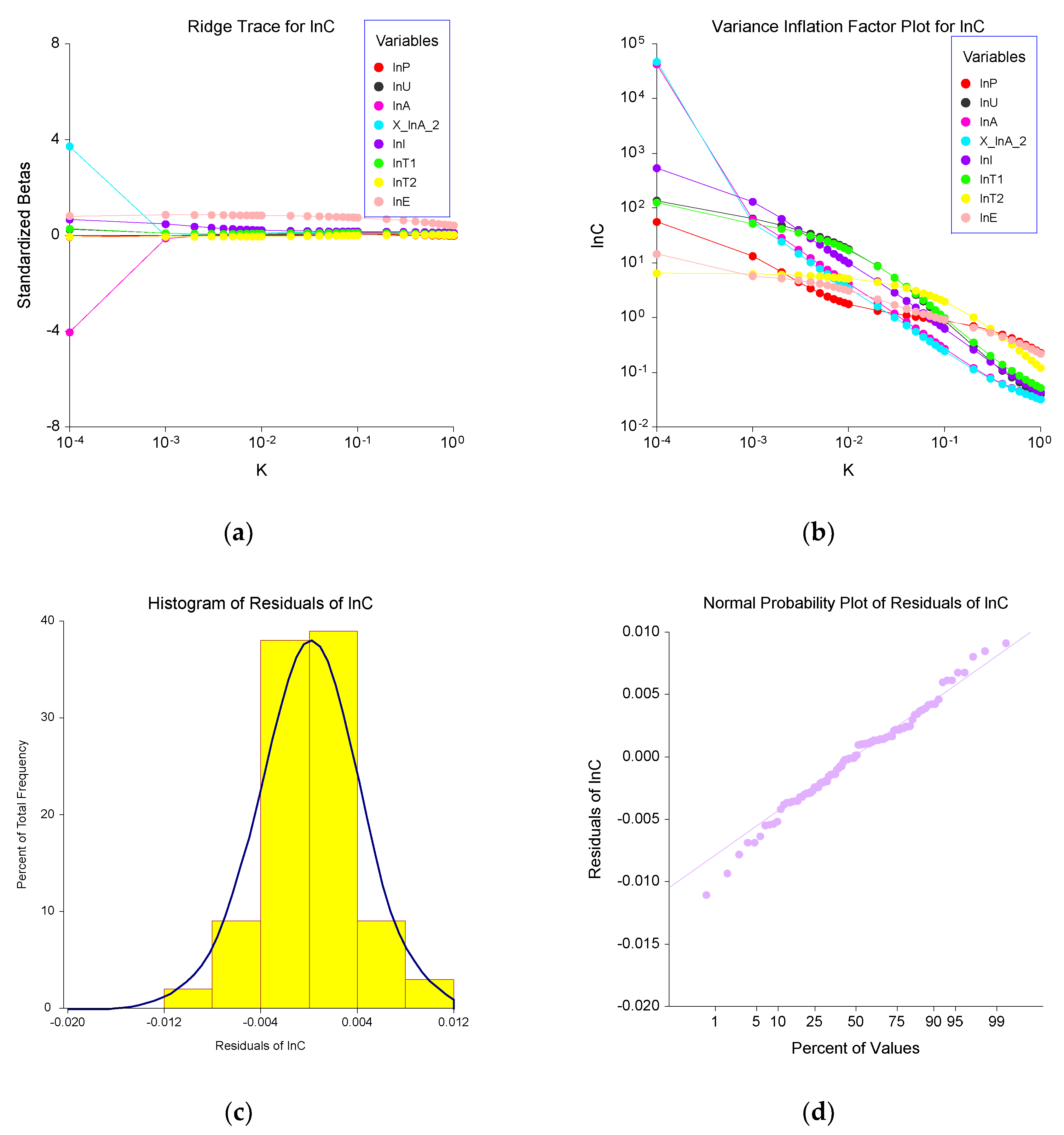
3.2. CO2 Forecast Model Based on Ridge Regression

Data availability was limited in this study, so we employed bootstrap random simulation to expand the sample size and increase the robustness of model estimation for small sample sizes [46]. The samples were analyzed and tested using ordinary least squares (Table 3), which indicated severe multicollinearity between the variables (i.e., the variance inflation factor (VIF) was larger than 10). In order to improve the stability of the estimated parameters, we used the ridge regression method, which is essentially an improved least squares estimation method. Ridge regression is a biased estimation regression method dedicated to collinear data analysis. It produces more realistic and reliable regression coefficients, but at the cost of losing some information and accuracy.
Based on the STIRPAT model, we obtained a formula for predicting CO2, as shown in Equation (13):
ln C = 0.8979279 + 0.07874562 × ln P + 0.03355597 × ln U + 0.03752399 × ln A + 0.0017604 × ( ln A ) 2     + 0.05296875 × ln I + 0.03148769 × ln T 1 + 0.00054033 × ln T 2 + 0.8248055 × ln E
The equation shows that, for every 1% change in the following indicators (population, urbanization, per capita GDP, industrial value-added, energy intensity, the carbon emission coefficient of the electric power sector, and coal consumption), CO2 emissions will increase by 0.07874562%, 0.03355597%, (0.03752399 + 0.001760419lnA)%, 0.05296875%, 0.03148769%, 0.000540327%, and 0.8248055%, respectively. Therefore, the order of the magnitude of the effect of the different indicators on CO2 emissions is: coal consumption > population > industrial value added > per capita GDP > urbanization > energy intensity > the carbon emission coefficient of the electric power sector.
Graphs of the ridge trace and the VIF plot show that, when k = 0.1, ridge trace changes tend to be stable, VIF tends to be stable, VIF approaches 1, and residual distribution conforms to a normal distribution (Figure 4). Analysis of variance (Table 4) produces the following results: R2 is equal to 0.926, the root mean square error (RMSE) is approximately 0.011, and the p-value of the variance analysis is 0.000. Therefore, the regression equation passes the significance test.

3.3. Forecast of CO2 Emissions

Predicted total CO2 emissions for the five scenarios in 2035 were sorted from high to low: BAU > IOD > MP > LCEP > ELC (Figure 5). The growth rate of energy-related CO2 emissions in Changxing slowed under all five scenarios. An annual growth rate of CO2 emissions ≥ 2% is a high speed, 1% ≤ CO2 emissions < 2% is a medium speed, 0 < CO2 emissions < 1% is a low speed, and CO2 emissions < 0 is a negative growth rate. The five scenarios can be classified into three CO2 growth rate categories, as follows.
(1)
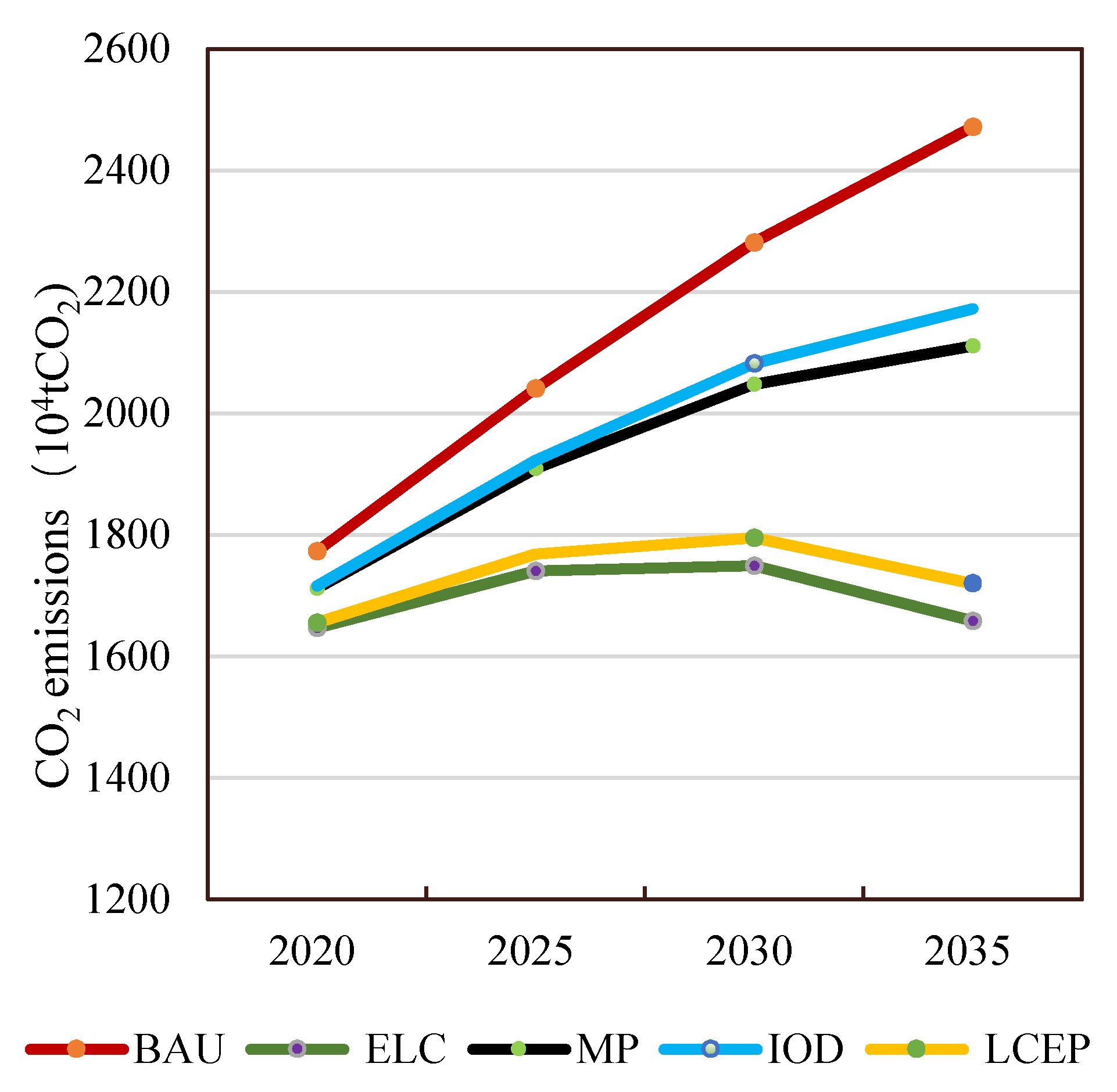
Under the BAU scenario, the growth rate of CO2 emissions is predicted to decrease from high speed (2018–2030) to medium speed (2031–2035). The annual growth rate of CO2 emissions will decrease from 4.10% in 2018 to 1.61% in 2035, but CO2 emissions in 2035 will still be 1.57 times the level in 2017, reaching 24.71 million tons. Under this scenario, although low-carbon technology has improved, Changxing cannot significantly reduce CO2 emissions during the outlook period if existing energy conservation and emissions reduction policies are extended without adopting stricter restraint measures.
(2)
The IOD and MP scenarios produced the same trend. The growth rate of CO2 emissions is expected to decrease from high speed (2018–2025) to medium speed (2026–2030) to low speed (2031–2035). In the IOD scenario, CO2 emissions in 2035 will reach 1.38 times the level in 2017, or 21.72 million tons, and will not peak during the outlook period. In the MP scenario, CO2 emissions in 2035 will reach 1.34 times the level in 2017, or 21.11 million tons, and will also not reach peak CO2. This suggests that even when the parameter settings are moderately constrained and total CO2 emissions are lower than the BAU scenario, peak CO2 cannot be reached during the outlook period.
(3)
The LCEP and ELC scenarios produced the same trend, with the growth rate of CO2 emissions predicted to decrease from medium speed (2018–2025) to low speed (2026–2030) to negative speed (2031–2035). In the LCEP scenario, CO2 emissions in 2035 will reach 1.09 times the level in 2017, or 17.19 million tons, which is equivalent to the level first reached in 2023. Peak CO2 emissions of 17.95 million tons are expected to occur in 2030, followed by an average annual decrease of −0.86%. In the ELC scenario, peak CO2 emissions of 17.49 million tons are expected to be reached in 2030, followed by an average annual decrease −1.06%. CO2 emissions in 2035 are predicted to be 1.06 times the level in 2017, reaching 16.58 million tons, which is equivalent to the level first reached in 2021. In these two scenarios, three parameters are the most constrained: coal consumption, energy intensity, and the carbon dioxide emission coefficient of the electric power sector. Equation (14) shows that the coefficient of coal consumption is the largest of the coefficients, which indicates that the impact of energy structure on CO2 emissions is absolutely dominant.
From 2018 to 2035, carbon intensity (at the 2010 constant-price GDP) in the five scenarios was predicted to decline to varying degrees. The predicted values for 2035, ranked from high to low, are: MP > ELC > BAU > LCEP > IOD (Figure 6). The carbon intensity of ELC is 2228.98 tCO2/USD, which is similar to that of MP (2270.72 tCO2/USD). Clearly, there is no advantage to the ELC approach. Despite producing the lowest CO2 emissions, ELC largely constrains the economic development of Changxing. IOD is expected to produce the lowest carbon intensity of 1661.02 tCO2/USD. However, the total amount of CO2 emissions expected in this scenario is relatively high. In other words, the IOD scenario sacrifices the environment to develop the county’s economy and is therefore not an appropriate development mode.
Considering carbon intensity and total carbon emissions, we found that LCEP is the most promising scenario for Changxing to achieve low-carbon development in the future. By 2035, carbon intensity under this scenario would be low (1849.69 tCO2/USD), which is lower than the peak CO2 levels reached by the United States in 2005. Moreover, under LCEP, the urbanization rate is expected to reach 76.54%, which is similar to the average urbanization level of 76.34% reached by other countries when they hit peak total carbon emissions, including the United States, Canada, Germany, the United Kingdom, and the European Union (Chai and Xu, 2015). In addition, industry’s share of GDP under the LCEP scenario drops to 37.73%, coal’s share of primary energy consumption drops to 56%, and the CO2 emission coefficient of the power sector drops to 3.95 tCO2/104 kWh. By 2030, per capita CO2 emissions in Changxing would reach 23.68 t, which is close to the peak of 22.2 t reached by the United States in 2005.

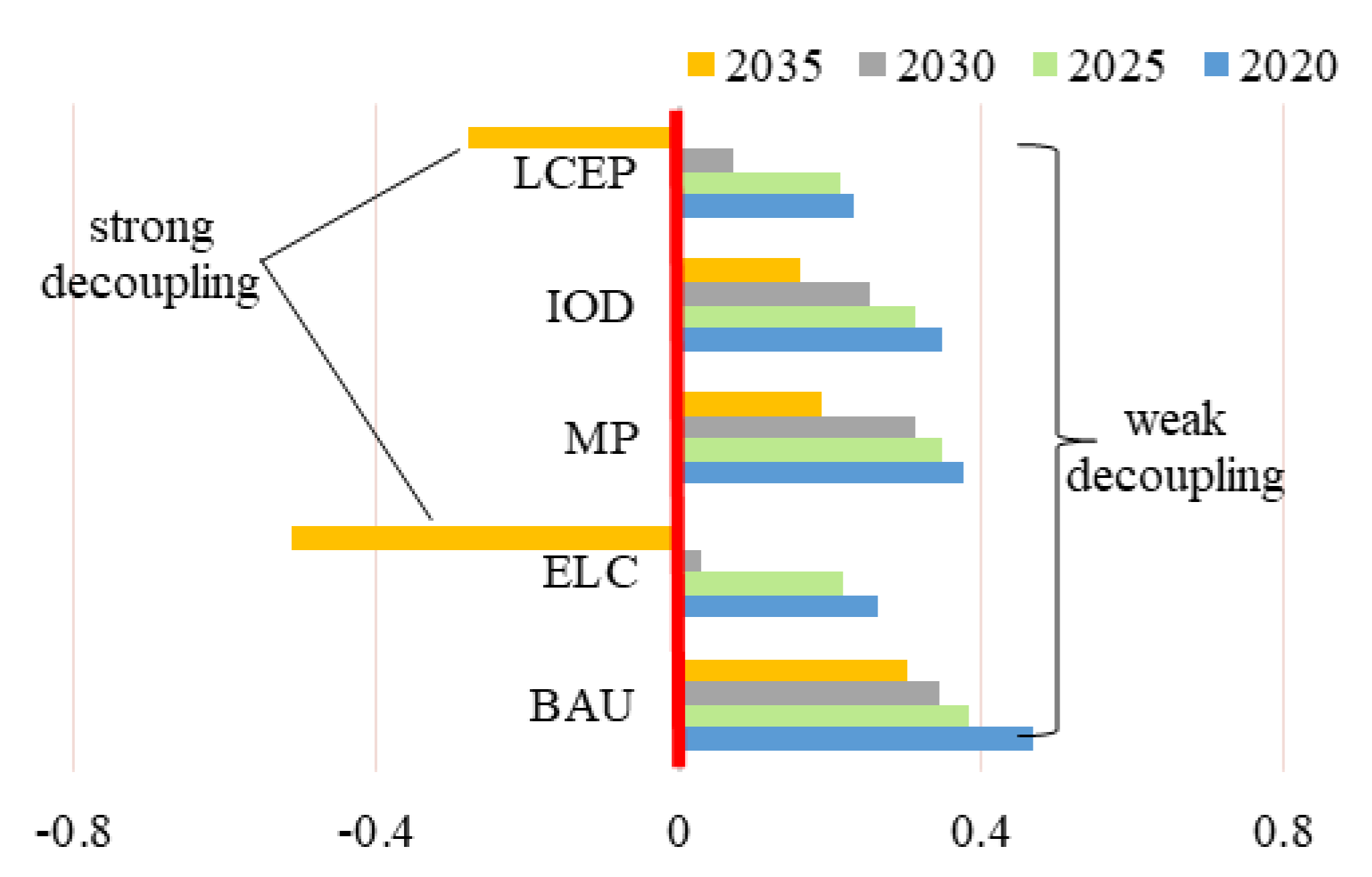
3.4. Relationship between CO2 Emissions and Economic Development

Overall, the degrees of coupling and decoupling of CO2 emissions growth (ΔCO2) from economic growth (ΔGDP) in Changxing experienced two phases, changing from strong decoupling (elasticity < 0) to weak decoupling (0 < elasticity < 0.8). Among them, abnormal results (expansive coupling and elasticity > 0.8) appeared in 2015, along with the large increase of CO2 emissions (Figure 7). It shows that with the economic growth, the environmental pressure is increasing, and the relationship between CO2 emissions and economic development is getting tense.
Under the five scenarios, we found that only in LCEP and ELC could Changxing achieve strong decoupling in 2035. However, in other scenarios, it remains weak decoupling (Figure 8). Hence, combined with the conclusion of Section 3.3, we provide abundant evidence to conclude that LCEP is the optimal strategy for Changxing to achieve low-carbon development. It shows that, to realize the decoupling of economic development and carbon emissions, two ways can be effective: optimizing energy structure and promoting low-carbon technological advancement.
For those industry-oriented regions similar to Changxing, we should give priority to optimizing the energy structure, especially by eliminating dependence on fossil fuels for power generation, to reduce CO2 emissions. Electricity decarbonization has been explored in the recent research [47,48]. On the other hand, the promotion of low-carbon technology is equally important. However, at the county scale, the development of low-carbon technology is also subject to marketing efforts, the transfer of intellectual property, and high input costs [49,50]. Therefore, counties are suggested to emphasize site-specific recommendations on exploring low-carbon technology, such as studying the possibility of energy recovery by thermal conversion of combustible residual materials or local agricultural and forestry waste, and focusing on one or two key techniques for reducing costs [51,52]. Besides, based on the results of decomposing drivers (Section 3.1), we also need to focus on optimizing the overall industrial structure and adjusting the internal industry sector to promote economic development while simultaneously inhibiting CO2 emissions. Other factors, such as urbanization population, are also important but not as critical for those regions. The growth of carbon emissions due to urbanization is limited because industry-oriented counties already have infrastructure that is mostly developed. In addition, such counties provide new employment opportunities for populations, which will be largely affected by the growth of emerging industries, the redevelopment of traditional pillar industries, and the closing of outdated or inefficient industries. This process will cause the size of floating populations to fluctuate, which then affects total population.
In the future scenarios, we emphasize the importance of both quantity (reducing fossil fuels consumption) and quality (promoting low-carbon technology) in low-carbon development. First to optimize the energy structure, especially in electric power sector, by significantly reducing dependency on fossil fuels. Some studies have shown that at the national scale, cutting CO2 emissions in electric power sector could be vital for achieving low-carbon society [53,54]. Not only that, in review of the literature, we found that nearly all industries are pursuing a rapid shift toward such a green transformation. Electrification of transportation at the larger scale is required for the road transport sector to achieve low-carbon mobility [55]. Transport structure adjustments and alternative fuels are required for the civil aviation sector to achieve decoupling [56]. The nonmetallic sector of Italy reduced 1.2 million tons of CO2 emissions between 1995 and 2009, benefiting from the cleansing of the energy structure (the share of conventional energy consumption declined by approximately 7%) [57]. Second to import/create core low-carbon technology, especially the integration of resource advantages and technical cooperation, Ubran [58] pointed out the importance of low-carbon technology in the further global political and economic power and considered that, in the energy sector (for example wind and solar energy), many firms and governments around the world are looking for partnerships and technology cooperation with China, as China can deliver advanced low-carbon technology at competitive prices. It not only helps to create new markets and employment but also accelerate global low-carbon transitions and climate change mitigation.

4. Conclusions

From the perspective of decomposing drivers, we found that optimizing the economic development mode and adjusting the energy structure of Changxing are key to slowing down CO2 emissions in the county during the outlook period. It was because of this that Dgdp was the most iconic factor driving CO2 emissions from 2010 to 2017, playing a long-term, direct, and dominant role, while Dmix had an inhibitory influence on CO2 emissions during most of the same period. Therefore, reducing the proportion of secondary industry (especially industry) and increasing the proportion of green industries emerged as the main factor capable of inhibiting CO2 emissions.
From the perspective of scenario/development strategy, a scenario focused on low-carbon development in the electric power sector (LCEP) is the optimal strategy for Changxing to achieve low-carbon development. This scenario is predicted to achieve the goal of peak CO2 emissions around 2030 with CO2 emissions per unit GDP lower than 2005 levels by 60%–65%, which meets China’s autonomous action goal declared to the UNFCCC.
Technology improvement and energy structure optimized are focused in LCEP scenario. Targeted measures for optimizing energy structure and promoting energy efficiency are proposed to ensure that Changxing reaches peak CO2 emissions as soon as possible. Such efforts include: (1) developing local support policies and regulations that guide the development of renewable energy in different areas, such as feed-in tariffs, renewable energy quotas, and fiscal tax support policies for the renewable energy power generation industry; (2) using advanced technologies to improve the energy efficiency of existing generators, including the production of supercritical and ultra-supercritical coal-fired power plants and the implementation of integrated gasification combined cycle power generation technology; and (3) increasing the proportion of non-fossil fuel power generation and accelerating the development of non-fossil fuel technologies based on biomass power generation and wind power to replace coal-fired power generation, while reducing the cost of new energy power generation.
The limitations of research using STIRPAT were presented in the parameter settings required for scenario analysis. Moreover, this method is a one-way information flow transmission that cannot dynamically reflect information interactions and lacks a feedback mechanism. Combining the method with the advantages of system dynamics might improve its flexibility and applicability to different scenarios.

Author Contributions

Conceptualization, Y.Q. and Q.Q.; Methodology, Y.Q.; Software, Y.Q. and L.S.; Validation, L.T. and Q.Q.; Investigation, Y.Q., X.S. and C.L.; Data Curation, X.S. and C.L.; Writing-Original Draft Preparation, Y.Q.; Writing-Review & Editing, Q.Q.; Funding Acquisition, Y.Q. and L.T. All authors have read and agreed to the published version of the manuscript.

Funding

This work was supported by the National Key R&D Program of China (2018YFC0704703 and 2017YFF0207303-2).

Acknowledgments

This work was supported by the National Key R&D Program of China (2018YFC0704703 and 2017YFF0207303-2).

Conflicts of Interest

The authors declare no conflict of interest.

References

  1. Houghton, J.T.; Meira Filho, L.G.; Callander, B.A.; Harris, N.; Kattenberg, A.; Maskell, K. Climate Change 1995: The Science of Climate Change: Contribution of Working Group I to the Second Assessment Report of the Intergovernmental Panel on Climate Change; Cambridge University Press: Cambridge, UK, 1996; Volume 2. [Google Scholar]
  2. Intergovernmental Panel on Climate Change. Climate Change 2013: The Physical Science Basis; Contribution of Working Group I to the Fifth Assessment Report; Intergovernmental Panel on Climate Change: Cambridge, UK; New York, NY, USA, 2013. [Google Scholar]
  3. National Development and Reform Commission. The Thirteenth Five-Year Plan. Available online: http://zys.ndrc.gov.cn/xwfb/201604/t20160429_800264.html (accessed on 19 January 2019).
  4. Zhou, Y. Decomposition of energy related CO2 emissions in China: A production-theoretical approach. Master’s Thesis, Xiamen University, Xiamen, China, 2014. [Google Scholar]
  5. Peng, Y.; Shi, C. Determinants of carbon emissions growth in China: A structural Decomposition analysis. Energy Proc. 2011, 5, 169–175. [Google Scholar] [CrossRef] [Green Version]
  6. Weinzettel, J.; Kovanda, J. Structural decomposition analysis of raw material consumption. J. Ind. Ecol. 2011, 15, 893–907. [Google Scholar] [CrossRef]
  7. Hermoso-Orzáez, M.J.; García-Alguacil, M.; Terrados-Cepeda, J.; Brito, P. Measurement of environmental efficiency in the countries of the European Union with the enhanced data envelopment analysis method (DEA) during the period 2005–2012. Environ. Sci. Pollut. Res. 2020. [Google Scholar] [CrossRef]
  8. Pasurka, C.A. Decomposing electric power plant emissions within a joint production framework. Energy Econ. 2006, 28, 26–43. [Google Scholar] [CrossRef]
  9. Fan, D. Driving factors of carbon emissions from energy consumption in China-based on LMDI-PDA method. China Environ. Sci. 2013, 33, 1705–1713. (In Chinese) [Google Scholar]
  10. Lin, B.; Du, K. Decomposing energy intensity change: A combination of index decomposition analysis and production-theoretical decomposition analysis. Appl. Energy 2014, 129, 158–165. [Google Scholar] [CrossRef]
  11. Wang, Q.; Chiu, Y.H.; Chiu, C.R. Driving factors behind carbon dioxide emissions in China: A modified production-theoretical decomposition analysis. Energy Econ. 2015, 51, 252–260. [Google Scholar] [CrossRef]
  12. Hatzigeorgiou, E.; Polatidis, H.; Haralambopoulos, D. CO2 emissions in Greece for 1990–2002: A decomposition analysis and comparison of results using the Arithmetic Mean Divisia Index and Logarithmic Mean Divisia Index techniques. Energy 2008, 33, 492–499. [Google Scholar] [CrossRef]
  13. Dhakal, S. Urban energy use and carbon emissions from cities in China and policy implications. Energy Policy 2009, 37, 4208–4219. [Google Scholar] [CrossRef]
  14. Geng, Y.; Zhao, H.; Liu, Z.; Xue, B.; Fujita, T.; Xi, F. Exploring driving factors of energy-related CO2 emissions in Chinese provinces: A case of Liaoning. Energy Policy 2013, 60, 820–826. [Google Scholar] [CrossRef]
  15. Sumabat, A.K.; Lopez, N.S.; Yu, K.D.; Hao, H.; Li, R.; Geng, Y.; Chiu, A.S.F. Decomposition analysis of Philippine CO2 emissions from fuel combustion and electricity generation. Appl. Energy 2016, 164, 795–804. [Google Scholar] [CrossRef]
  16. Xu, S.; He, Z.; Long, R.; Chen, H.; Han, H.; Zhang, W. Comparative analysis of the regional contributions to carbon emissions in China. J. Clean Prod. 2016, 127, 406–417. [Google Scholar] [CrossRef]
  17. Miao, W.; Chao, F. Decomposition of energy-related CO2 emissions in China: An empirical analysis based on provincial panel data of three sectors. Appl. Energy 2017, 190, 772–787. [Google Scholar]
  18. Ang, B.W.; Liu, N. Energy decomposition analysis: IEA model versus other methods. Energy Policy 2007, 35, 1426–1432. [Google Scholar] [CrossRef]
  19. Ang, B.W.; Zhang, F.Q.; Choi, K.H. Factorizing changes in energy and environmental indicators through decomposition. Energy 1998, 23, 489–495. [Google Scholar] [CrossRef]
  20. Xu, X.; Ang, B.W. Index decomposition analysis applied to CO2 emission studies. Ecol. Econ. 2013, 93, 313–329. [Google Scholar] [CrossRef]
  21. Sangeetha, A.; Amudha, T. A novel bio-inspired framework for CO2 emission forecast in India. Proc. Comput. Sci. 2018, 125, 367–375. [Google Scholar] [CrossRef]
  22. Chai, Q.; Xu, H. Modeling carbon emission peaking pathways in China based on integrated assessment model IAMC. China Popul. Resour. Environ. 2015, 25, 37–46. (In Chinese) [Google Scholar]
  23. Nieves, J.A.; Aristizábal, A.J.; Dyner, I.; Báez, O.; Ospina, D.H. Energy demand and greenhouse gas emissions analysis in Colombia: A LEAP model application. Energy 2019, 169, 380–397. [Google Scholar] [CrossRef]
  24. Manne, A.S.; Wene, C.O. MARKAL-MACRO: A Linked Model for Energy-Economy Analysis, BNL-47161 Report; Brookhaven National Lab: Upton, NY, USA, 1992. [Google Scholar]
  25. Zhou, P.; Zhou, X.; Zhou, D.Q. A survey of estimating CO2 mitigation costs. Manag. Rev. 2014, 26, 20–27. (In Chinese) [Google Scholar]
  26. Ding, S.; Dang, Y.G.; Li, X.M.; Wang, J.J.; Zhao, K. Forecasting Chinese CO2 emissions from fuel combustion using a novel grey multivariable model. J. Clean. Prod. 2017, 162, 1527–1538. [Google Scholar] [CrossRef]
  27. Hong, T.; Jeong, K.; Koo, C. An optimized gene expression programming model for forecasting the national CO2 emissions in 2030 using the metaheuristic algorithms. Appl. Energy 2018, 228, 808–820. [Google Scholar] [CrossRef]
  28. Ehrlich, P.; Ehrlich, A. The Population Explosion; Simon & Schuster Inc.: New York, NY, USA, 1990. [Google Scholar]
  29. Dietz, T.; Rosa, E.A. Rethinking the environmental impacts of population, affluence and technology. Hum. Ecol. Rev. 1994, 1, 277–300. [Google Scholar]
  30. Wang, Z.; Wei, L. Determinants of CO2 emissions from household daily travel in Beijing, China: Individual travel characteristic perspectives. Appl. Energy 2015, 158, 292–299. [Google Scholar] [CrossRef]
  31. Xu, B.; Lin, B. Reducing carbon dioxide emissions in China’s manufacturing industry: A dynamic vector autoregression approach. J. Clean. Prod. 2016, 131, 594–606. [Google Scholar] [CrossRef]
  32. Department of Rural Socio-Economic Survey, National Bureau of Statistics of China. China Statistical Yearbook (County-Level); China Statistics Press: Beijing, China, 2016.
  33. Cai, B.F. Study on CO2 emissions of China cities. Energy China 2011, 33, 28–32. (In Chinese) [Google Scholar]
  34. National Bureau of Statistics of China. China Statistical Yearbook 2016; China Statistics Press: Beijing, China, 2016. Available online: http://www.stats.gov.cn/ (accessed on 30 April 2019).
  35. Statistical Bureau of Changxing County. Changxing Statistical Yearbook (2010–2017). Available online: http://www.zjcx.gov.cn/ (accessed on 30 April 2019).
  36. Zhejiang Province Economic and Information Commission, Zhejiang Province Bureau of Statistic. Energy and Utilization in Zhejiang Province in 2015 (White Paper). Available online: http://www.zjjxw.gov.cn/ (accessed on 30 April 2019).
  37. Ang, B.W. The LMDI approach to decomposition analysis: A practical guide. Energy Policy 2005, 33, 867–871. [Google Scholar] [CrossRef]
  38. York, R.; Rosa, E.A.; Dietz, T. Stirpat, Ipat and Impact: Analytic tools for unpacking the driving forces of environmental impacts. Ecol. Econ. 2003, 46, 351–365. [Google Scholar] [CrossRef]
  39. Yan, H.; Guo, Y.; Lin, F. Analyzing the Developing Model of Chinese Cities under the Control of CO2 Emissions Using the STIRPAT Model: A Case Study of Shanghai. Acta Geogr. Sin. 2010, 65, 983–990. (In Chinese) [Google Scholar]
  40. Central Committee of the Communist Party of China. Communique of the 5th Plenary Session of the 18th Central Committee of Communist Party of China; People’s Publishing House: New Delhi, India, 2015; pp. 1–26.
  41. National Bureau of Statistics of China. China Statistical Yearbook 2018; China Statistics Press: Beijing, China, 2018. Available online: http://www.stats.gov.cn/ (accessed on 4 July 2019).
  42. Institute of Urban Science, Shanghai Jiaotong University, China Urban Research Center of Beijing Jiaotong University. 2016–2020 China Urbanization Rate Growth Forecast Report. Available online: http://urban.people.cn/n1/2016/1230/c397284-28990381.html/ (accessed on 4 July 2019).
  43. Jian, X.; Huang, K. Empirical analysis and forecast of the level and speed of urbanization in China. Econ. Res. J. 2010, 3, 28–39. (In Chinese) [Google Scholar]
  44. The World Bank and Development Research Center of the State Council PRC. China 2030: Building a Modern, Harmonious, and Creative Society. Available online: http://www.drc.gov.cn/download/2874407/29 (accessed on 4 July 2019).
  45. The People’s Government of Changxing County, Zhejiang Province. The Thirteenth Five-Year Plan of Changxing County. Available online: http://www.zjcx.gov.cn/ (accessed on 4 July 2019).
  46. Efron, B. Bootstrap methods: Another look at the Jackknife. In Breakthroughs in Statistics: Methodology and Distribution; Kotz, S., Johnson, N.L., Eds.; Springer: New York, NY, USA, 1992; pp. 569–593. [Google Scholar]
  47. Barido, D.P.D.L.; Avila, N.; Kammen, D.M. Exploring the enabling environments, inherent characteristics and intrinsic motivations fostering global electricity decarbonization. Energy Res. Soc. Sci. 2020, 61. [Google Scholar] [CrossRef]
  48. Burandt, T.; Xiong, B.; Löffler, K.; Oei, P.Y. Decarbonizing China’s energy system—Modeling the transformation of the electricity, transportation, heat, and industrial sectors. Appl. Energy 2019, 255. [Google Scholar] [CrossRef]
  49. Jiang, Y.; Fan, L.; Shi, G. Study on the current situation and barriers of China’s low carbon technology. Ecol. Econ. 2014, 30, 47–52. (In Chinese) [Google Scholar]
  50. Zhou, Y.; Zou, J.; Wang, K. How can low-carbon technologies break through bottlenecks of the intellectual property? Environ. Prod. 2010, 68–70. (In Chinese) [Google Scholar]
  51. Carmo-Calado, L.; Hermoso-Orzáez, M.J.; Mota-Panizio, R.; Guilherme-Garcia, B.; Brito, P. Co-Combustion of Waste Tires and Plastic-Rubber Wastes with Biomass Technical and Environmental Analysis. Sustainability 2020, 12, 1036. [Google Scholar] [CrossRef] [Green Version]
  52. Beims, R.F.; Hu, Y.; Shui, H.; Xu, C. Hydrothermal liquefaction of biomass to fuels and value-added chemicals: Products applications and challenges to develop large-scale operations. Biomass Bioenergy 2020, 135. [Google Scholar] [CrossRef]
  53. Liao, C.; Wang, S.; Fang, J.; Zheng, H.; Liu, J.; Zhang, Y. Driving forces of provincial-level CO2 emissions in China’s power sector based on LMDI method. Energy Proc. 2019, 158, 3859–3864. [Google Scholar] [CrossRef]
  54. Barton, J.; Davies, L.; Dooley, B.; Foxon, T.J.; Galloway, S.; Hammond, G.P.; O’Grady, Á.; Robertson, E.; Thomson, M. Transition pathways for a UK low-carbon electricity system: Comparing scenarios and technology implications. Renew. Sustain. Energy Rev. 2018, 82, 2779–2790. [Google Scholar] [CrossRef] [Green Version]
  55. Vaidya, B.; Mouftah, H.T. Connected autonomous electric vehicles as enablers for low-carbon future. In Research Trends and Challenges in Smart Grids; IntechOpen: London, UK, 2019. [Google Scholar] [CrossRef] [Green Version]
  56. Yu, J.; Shao, C.; Xue, C.; Hua, H. China’s aircraft-related CO2 emissions: Decomposition analysis, decoupling status, and future trends. Energy Policy 2020. [Google Scholar] [CrossRef]
  57. Wang, J.; Liao, H.; Tang, B.; Ke, R.; Wei, Y. Is the CO2 emissions reduction from scale change, structural change or technology change? Evidence from non-metallic sector of 11 major economies in 1995–2009. J. Clean. Prod. 2017, 148, 148–157. [Google Scholar] [CrossRef]
  58. Urban, F. China’s rise: Challenging the north-south technology transfer paradigm for climate change mitigation and low carbon energy. Energy Policy 2018, 113, 320–330. [Google Scholar] [CrossRef]
Figure 1. Technical route of the research.
Energies 13 01212 g001
Figure 2. Comparison of the changes in Dtot and CO2 emissions. Dtot: the total effect of six driving factors.
Energies 13 01212 g002
Figure 3. Trends of six driving factors influencing CO2 emissions based on the Logarithmic Mean Divisia Index (LMDI) decomposition. Dpop: population scale effect, Dgdp: economic output effect, Dstr: industrial structure effect, Dint: energy intensity effect, Dmix: energy mix effect, and Demf: carbon emission coefficient effect. (a) Dpop. (b) Dgdp. (c) Dstr. (d) Dint. (e) Dmix. (f) Demf.
Energies 13 01212 g003
Figure 4. Ridge regression report. (a) Ridge trace for lnC, (b) variance inflation factor (VIF) plot for lnC, (c) histogram of lnC residuals, and (d) normal probability plot of lnC residuals. C: CO₂ emissions. lnC: the logarithmic form of C.
Energies 13 01212 g004
Figure 5. CO2 emissions forecast for Changxing County. BAU: business as usual, ELC: enhanced low-carbon, MP: moderate progressive, IOD: industry-oriented development, and LCEP: low-carbon development in the electric power sector.
Energies 13 01212 g005
Figure 6. CO2 emissions intensity forecast for Changxing County.
Energies 13 01212 g006
Figure 7. Degrees of coupling and decoupling of CO2 emissions growth (ΔCO2) from economic growth (ΔGDP) for Changxing County from 2011 to 2017.
Energies 13 01212 g007
Figure 8. Degrees of decoupling of CO2 emissions growth (ΔCO2) from economic growth (ΔGDP) for Changxing County in five scenarios.
Energies 13 01212 g008
Table 1. Parameter levels used in five scenarios.
BAUELCMPIODLCEP
Growth rate of populationMMMMM
Growth rate of urbanizationMMMMM
Growth rate of GDPHLMHM
Decline rate of industrial proportion LHMLM
Decline rate of energy intensityMHMHH
Decline rate of CO2 emission coefficient of electric power sectorLHMMH
Decline rate of coal consumptionMHMMH
Note: “L”, “M,” and “H” represent low, medium, and high parameter levels, respectively. Five scenarios are established, including business as usual (BAU), enhanced low-carbon (ELC), moderate progressive (MP), industry-oriented development (IOD), and low-carbon development in the electric power sector (LCEP).
Table 2. Parameter settings in low (L), medium (M), and high (H) speed development conditions.
2018–20202021–20252026–20302031–2035
LMHLMHLMHLMH
Growth rate of population0.41%0.47%0.55%0.17%0.24%0.31%−0.09%−0.01%0.04%−0.28%−0.20%−0.14%
Growth rate of urbanization2.45%3.64%5.34%1.45%2.14%2.84%0.95%1.64%2.34%0.45%1.14%1.84%
Growth rate of GDP6.50%8.50%9.65%5.90%7.30%8.75%4.10%5.00%7.55%2.30%3.50%6.05%
Decline rate of industrial proportion −1.57%−2.07%−2.57%−1.07%−1.57%−3.57%−0.57%−1.07%−3.57%−0.27%−1.57%−3.57%
Decline rate of energy intensity−4.39%−7.26%−8.31%−4.00%−6.00%−7.00%−3.50%−5.00%−6.00%−3.00%−4.00%−5.00%
Decline rate of CO2 emission coefficient of electric power sector−3.64%−4.14%−5.04%−3.64%−4.14%−5.04%−3.64%−4.14%−5.04%−3.64%−4.14%−5.04%
Proportion of coal in primary energy consumption80.00%77.00%74.00%75.00%70.00%64.00%70.00%63.00%54.00%65.00%56.00%44.00%
Table 3. Least squares multicollinearity.
Independent VariableVariance InflationR-Squared vs. Other X’sTolerance
lnP56.01280.98210.0179
lnU136.80430.99270.0073
lnA42,475.410
(lnA)246,913.2110
lnI535.58840.99810.0019
lnT1126.22880.99210.0079
lnT26.4270.84440.1556
lnE14.3950.93050
Note: P: population, U: urbanization, A: affluence (expressed as per capita GDP), I: industrial value added, T1: technology (expressed as energy intensity), T2: technology (expressed as carbon emission coefficient of the electric power sector), and E: energy consumption. Take the logarithmic form for all the independent variables.
Table 4. Analysis of variance for k = 0.1.
SourceDegree of
Freedom
Sum of
Squares
Mean
Square
F-RatioProb Level
Intercept15262.1045262.104
Model80.1317190.01646488142.38760.000000
Error910.010522720.0001156342
Total(Adjusted)990.14224180.001436785
Mean of Dependent7.254036
Root Mean Square Error0.01075334
R-Squared0.9260
Coefficient of Variation0.001482393

