An Interval-Arithmetic-Based Approach to the Parametric Identification of the Single-Diode Model of Photovoltaic Generators

Abstract

Parametric identification of the single diode model of a photovoltaic generator is a key element in simulation and diagnosis. Parameters’ values are often determined by using experimental data the modules manufacturers provide in the data sheets. In outdoor applications, the parametric identification is instead performed by starting from the current vs. voltage curve acquired in non-standard operating conditions. This paper refers to this latter case and introduces an approach based on the use of interval arithmetic. Photovoltaic generators based on crystalline silicon cells are considered: they are modeled by using the single diode model, and a divide-and-conquer algorithm is used to contract the initial search space up to a small hyper-rectangle including the identified set of parameters. The proposed approach is validated by using experimental data measured in outdoor conditions. The information provided by the approach, in terms of parametric sensitivity and of correlation between current variations and drifts of the parameters values, is discussed. The results are analyzed in view of the on-site application of the proposed approach for diagnostic purposes.

1. Introduction

Photovoltaic (PV) array modeling is crucial in many fields, including the prediction of energy production [1], the design, the control [2] and the diagnosis [3]. The increase of the PV cells would be desirable, in a context where many types of technologies have been developing, although 90%–95% of the market is still dominated by mono-crystalline and poly-crystalline silicon technologies [4]. The mono-crystalline PV commercial modules reach efficiencies between 15% and 22%; meanwhile, poly-crystalline technology goes up to the efficiency range of 14%–20%. The economies of scale of its main material, silicon, make crystalline silicon cells more affordable and highly efficient compared to other materials [5]. Other technologies derived from crystalline silicon technologies have been gaining importance in the research and commercial fields, such as half-cell, double glass and bifacial [4]. On the other hand, thin film technologies, e.g., amorphous silicon, CdS/CdTe and CIS, represent close to 5%–10% of the market [4]. Emerging technologies, e.g., organic and perovskite ones, offer interesting perspectives in terms of efficiency [6], but some barriers still need to be overcome, especially durability and price [5]. The approach proposed in this paper refers to PV generators based on crystalline silicon cells, which represent the largest part of the market. Different models have been studied in the scientific publications to represent PV modules based on crystalline silicon cells. The single diode model (SDM) offers a reasonable trade-off between accuracy and degree of non linearity, such that it is widely used in literature. It involves five parameters, which are related to the photo-induced current, the P-N junction and the losses. These parameters are in turn dependent on other ones related to the cell material and the environmental conditions—the irradiance and the temperature; see [7,8]. The double diode model (DDM) allows one to model the dark current losses and the effect of pair generation—recombination in the space charge region [9], but at the cost of an increase in the number of parameters, increasing from five for the SDM, to seven. A more complicated model can be used in a case where the PV cells’ behavior at negative voltage values has to be accounted for. A further generator is included in this model [10], so that the parameters required become eight.

In this paper, the SDM is preferred to the DDM because of the features mentioned above and also because the PV array working conditions considered are uniform; thus, the model proposed in [10] becomes superfluous. A key operation for an accurate SDM-based simulation of the PV array is the identification of the five model parameters. This is very often done by employing data that are provided by the PV module manufacturer through the data sheet. These experimental measurements refer to a specific operating conditions of the cells, called standard test conditions (STC).

In the literature, parametric identification is done by using analytical methods or fitting techniques [11]. In

Table 1. Comparison among different approaches to parametric identification of SDM.

Methods/ Features	Core of the Procedure	Implemen- Tation Complexity	Speed Conver- Gence	Robustness with Noisy Data	Initial Condition Impact	Require- Ment of Algorithm Setting
Analytical	Set of equations solved explicitly	Low	High	Medium	High	Medium
Iterative non-linear minimization	Equations must be solved by numerical methods	High	Low	Medium	High	Low
Heuristics	Fitting I-V curve model to measured data by a soft computing algorithm	High	Medium	Medium	High	High
Hybrids	Combining non-linear minimization and heuristics	High	Medium/ Low	Medium	High	High
Proposed IA Based $D\&C$	Parameters are intervals divided and tested using feasibility conditions	Low	Medium/ High	High	Low	Low

a comparison among such approaches is given by referring to the implementation complexity, the convergence speed, the robustness when noisy data are considered, the impact of the initial conditions and the requirements of algorithmic setting. Analytical approaches are based on a set of simplified equations leading to explicit formulas allowing one to calculate the five parameters of the SDM without using any iterative method [12]. Some approaches consider the SDM lossless model, or scale down the order of the SDM by considering an infinite value of the shunt resistance or by neglecting the series resistance [13]. The most common simplification consists of supposing that the short-circuit current ($I_{sc}$) value is equal to the photo-induced current ($I_{ph}$) [14]. A set of equations is derived at the main points of the current vs. voltage (I-V) curve: at the maximum power point (MPP), at the short circuit operating point through $I_{sc}$ and in open circuit conditions through $V_{oc}$. Noisy I-V data may have a significant effect on parameters values. This is the case, for instance, for a series and for the shunt resistances whose values are related to the slopes of the I-V curve in an open circuit and in short circuit conditions, respectively. Additionally, the so called translation equations have been considered in some papers to relate the I-V curve in non-standard conditions to the five SDM parameters that are scaled according to the irradiance and temperature conditions the I-V curve refers to [14,15,16,17,18]. Simplified and direct equations make the implementation of the method suitable, even for an embedded processor, at the cost of a reduced accuracy.

Many other approaches to the SDM parametric identification are based on optimization methods, which are usually aimed at the root mean square error (RMSE) between the simulated I-V curve and the experimental curve minimization. The convergence of the algorithm depends on factors such as the guess condition, the objective function and the algorithm itself. Three main approaches are proposed: the one using non-linear minimization algorithms [19,20], the one using heuristics approaches [21,22,23,24] and the adoption of hybrid methods [25]. The non-linear algorithms are computationally expensive [19,20], but that allows for solving numerically, the set of non-linear equations of SDM. In [20], Matlab embedded Levenberg–Marquardt and Gauss-Newton nonlinear equation solvers were used to manage the SDM equations. The parameters in STC were obtained from modules’ data sheets, and translation equations [15,16] were used to obtain the SDM model in other operating conditions. Noisy data affect the confidence intervals of the solutions achieved by these algorithms. The termination conditions and the related parameters have to be chosen in order to have a trade-off between computation time and accuracy. Low values of the convergence thresholds and high values assigned to the maximum number of iterations are compatible with off-line identification purposes. Moreover, the iterative methods, such as Newton methods, are less complex, but they might be trapped in local optima and show a high dependency from the guess solution used. For instance, in [26] $R_s$ is neglected, so that four equations to determine four SDM parameters are proposed, the series resistance value being fitted by calculating the power error between the SDM and the experimental measurements in a iterative way. Nonlinear minimization algorithms are often used to fit I-V experimental curves, the objective function to minimize being the error between the model and experimental data. Trust-region and Levenberg-Marquardt methods are widely used, but they require a good guess solution. Simulation platforms, e.g., Matlab and Mathematica, provide curve fitting tools to perform offline parametric identification. Recently, soft computing methods, such as artificial neural networks [21,22], genetic algorithms [23] and particle swarm optimization (PSO) [23], among others, have been employed more and more frequently. Such approaches are not suitable for online operation because of the computational complexity of the stochastic algorithms. The approaches introduced in [21,22] operate on suitable sets of I-V curves, related to a specific module’s operation, to train neural networks. To determine the amount of training data and the numbers of layers and neurons is a challenging task. In genetic algorithms [23], fixing selection, reproduction and mutation operators and values of the related parameters is challenging as well. Settings such as population size, iteration number and mutation rate, among others, have to be well adjusted to prevent the algorithm from stalling. Therefore, in terms of setting of the heuristic algorithms, several initial guess values have to be designed by an expert and/or through a trial and error procedure. By combining different techniques, some weaknesses are reduced. For example, in [25] the global exploration capabilities of the soft computing algorithm artificial bee colony (ABC) allowed it to reduce the space for exploring solutions, and local searching was done by the trust-region reflective algorithm, thereby improving accuracy, convergence and reliability. Unfortunately, there is not a consensus about the improvement of the computation time achieved by hybrid approaches.

The difficulty of the parametric identification comes from the high non linearity of the SDM and from the fact that the values of the parameters have very different orders of magnitude. With respect to the identification performed on the basis of the STC experimental data that are usually available in PV modules data sheets, the parametric identification using data acquired while the PV module is working in outdoor conditions show different features. Indeed, the whole I-V curve is usually available and irradiance (G) and temperature (T) values at which the PV module is working might be also given.

Interval arithmetic (IA) is a mathematical approach that is used in many contexts for evaluating the propagation of the uncertainty affecting input data on the output of a given system. Moreover, it has been used for tolerance analysis and design in the context of electrical and electronic engineering; e.g., in [27,28,29]. By IA, parameters assume values that are not real numbers, but intervals limited by a lower and an upper bound: in an interval the parameter may assume any value with the same probability. In [28] an evolutionary approach to worst case tolerance design of magnetic devices is presented. The algorithm improves on the classical nominal design, accounting for parameter variations and tolerances, so that the system performance does not exceed upper and lower specifications imposed in advance by the designer. In [27], IA is used to perform tolerance analysis and design and to evaluate the production yield. In [29], an IA based estimation state in power distribution networks with high penetration of photovoltaic generators is proposed. In this case, IA is adopted to deal with measurement uncertainty. The proposed method allows one to determine the upper and lower bounds of state variables, which is helpful for providing operators the confidence that the actual value variable is not exceeding the voltage security constraint, thereby improving the network operation for the case of uncertain inputs.

IA-based parametric identification has never been used in the outdoor PV context, but it can be helpful for designing an algorithm profiting from IA features, thereby giving a reliable result with little computational effort. The IA based approach presented in this paper starts from a large volume in the parameter search space and contracts it by means of a divide-and-conquer ($D\&C$) strategy up to converge to a tight hyper-rectangle including the experimental measurements in the I-V plane. The proposed IA based $D\&C$ algorithm requires the user to fix the initial intervals for the five SDM parameters and two thresholds for the feasibility and the termination conditions respectively. The initial intervals, which define the search parameters’ space, are contracted towards the identified set, if they are included in the search space. Otherwise, the IA based $D\&C$ algorithm informs the user about the guaranteed infeasibility of the whole search space. To fix the search space is obviously easier for a not-so-skilled user than to provide a guess solution that is quite close to the final one, as is required by gradient-based minimization approaches. This feature is very helpful, especially for some parameters, e.g., saturation current and thermal voltage, that greatly depend on cells material and on operating conditions. As for the feasibility condition, the desired amount of experimental data contained in the IA computed I-V boundaries depends on the application, and it can be fixed as greater than 85%. In the same way, the threshold to fix in the termination condition is chosen as the desired resolution of the interval solution. $D\&C$ strategy allows one to evaluate solutions separately, so parallel computing is suitable to decrease the computation time without sacrificing the size of search space. This is a distinctive feature compared to the other approaches, which in general have to make a compromise between accuracy and computation time.

The paper is organized as follows: In the first section an introduction of SDM is done. Then, IA theory is briefly recalled and it is applied to the SDM. Later on, $D\&C$ algorithm is presented. In Section 4, the proposed method using IA and $D\&C$ algorithm is detailed. In Section 5, the results obtained to estimate $R_s$, $R_h$, $I_{sat}$, B and $I_{ph}$ parameters of the SDM model are analyzed. The sixth section proposes a discussion about the results presented in the paper and closes with the conclusions.

2. Photovoltaic Generator Single Diode Model

Figure 1 shows the SDM circuit: it includes the photoinduced current generator $I_{ph}$, which models the photovoltaic effect; a diode D modeling the P-N junction; and the resistances $R_s$ and $R_h$ representing the ohmic losses and the recombination losses respectively. Thus, the following five parameters appear in the model:

$I_{sat,d}$: saturation current in the P-N junction;

$I_{ph}$: photo-induced current;

$R_s$: series resistance;

$R_h$: parallel resistance;

B: it includes the ideality factor n, which is the fifth parameter to be identified. It is: $B=N_s·n·k·T/q$, where $N_s$ is the number of series connected cells, T is the cells operating temperature, k is the Boltzmann constant and q is the electron charge.

It is worth noting that the five parameters mentioned above show some dependencies from physical parameters that are typical of the semiconducting material used for the cells’ fabrication and also from irradiance G and temperature T. As in the majority of the literature concerning I-V curve based parametric identification, in this paper also, the identification focuses on the five parameters mentioned above, thereby neglecting their dependencies on other physical parameters. This further correlation, and the dependency on G and T especially, can be exploited after having identified the set $\{I_{sat,d},I_{ph},R_s,R_h,B\}$ to the aim of having, in turn, the values of the physical parameters, including G and T.

The output current I of the PV array is obtained by combining the Kirchhoff voltage and current laws and the characteristic equations of the components appearing in the SDM.

$$I=I_{ph}-I_d-I_h$$

(1)

$$I_d=I_{sat,d}(e^{V_d/B}-1)$$

(2)

$$V_d=V+R_s·I$$

(3)

$$I_h=\frac{V_d}{R_h}=\frac{V+R_s·I}{R_h}$$

(4)

In [30] it is shown that the resulting function expressing the relationship between the current I and the voltage V at the PV generator terminals is implicit, but the Lambert W-function is useful for achieving an explicit non-linear relation between I and V, which is given in (5).

$$I=\frac{R_h(I_{ph}+I_{sat,d})-V}{R_h+R_s}-\frac{B}{R_s}LambertW\left(\theta \right)$$

(5)

wherein: $\theta =\left\{(R_s//R_h)I_{sat,d}{e}^{\left[(R_h{R}_s(I_{ph}+I_{sat,d})+R_{h}V)/B(R_h+R_s)\right]}\right\}/B$.

Later on, without loss of generality, the discussion is referred to one PV module. The set of unknown five parameters is $P=\{I_{sat,d},I_{ph},R_s,R_h,B\}$.

In Figure 2 a PV module I-V curve is shown by blue marks: it has been obtained by placing the values listed in

Table 2. STC Parameters for a 140 W PV Yingli solar panel.

Parameter	Meaning	Value
$I_{sat,d}$[A]	Saturation current in cell	5.359647 $\times {10}^{-10}$
$I_{ph}$[A]	Photoinduced current	8.3
$R_s[\Omega ]$	Series resistance	0.1793
$R_h[\Omega ]$	Shunt resistance	150.70
B	$N_s·n·k·T/q$	1.0532

into Equation (5). The parameters in Table 2 refer to a 140 W PV Yingli solar panel working in STC, which have been obtained by the method proposed in [31] in STC. This PV module consists of 36 polycrystalline solar cells connected in series. In the same figure, the I-V curves corresponding to 30% variations of the parameters $R_s$, $R_h$, $I_{sat}$ and B are also shown in magenta, cyan, red and black respectively. The I-V curve exhibits a significant sensibility with respect to variations of B and $I_{sat}$ in proximity to the MPP and a dependency on $R_s$ in the high voltage range. The parameter $I_{ph}$ depends on, almost directly, irradiance, and its value is usually assumed to be equal to the short-circuit current [2].

In the literature, SDM parametric identification of the parameters has been often addressed by minimization algorithms, which are aimed at fitting the experimental I-V curve with the one generated by the SDM. The result is a set of five real values, one for each of the five parameters in the SDM (Table 2). IA, instead, should be used to identify the parameters by starting from the I-V curve, and by exploiting the IA properties, guaranteeing that the I-V ranges correspond to the set of parameters bound to the experimental measurements. Later on, the main IA features and properties are recalled in order to appreciate how they are suitably exploited in the PV parametric identification context.

3. Interval Arithmetic for I-V Curve Representation

The basic mathematical entity used in IA is the interval. Thus, the parameters appearing in the model can be treated as intervals $\left[X\right]$ instead of real numbers X. The approach consists of treating parameters or variables as having ranges of values, instead of discrete values. The bounds of the interval $\left[X\right]$, using the nomenclature proposed in the IEEE Std 1788.1 [32], are called $\underline{x}$ and $\overline{x}$. Thus, $\left[X\right]$ = $[\underline{x}$, $\overline{x}]$; it is defined by $x=\left\{x\in \Re /\underline{x}\le x\le \overline{x}\right\}$. Basic arithmetic operations among interval variables are well defined in the IA foundations [33]. The operation among two intervals results in an interval too, having the property that it contains all the possible results obtained by the combination of all the values included in the intervals corresponding to the operands. The values in the intervals are assumed to have the same probability of occurring, so that the probabilities of the values are uniform. This means that all the values in $\left[X\right]$ are equi-probable. IA theory also shows that the simple representation of the operands, which consists of the lower and of the upper bound of the intervals thereof, does not allow one to take into account any correlation among the variables. As a consequence of this, the IA result is an over-estimation of the true range of the result. This means that the IA result is guaranteed to contain all the possible results of the operation, but the over-estimation might be too much wider than the real interval. In order to reduce this IA drawback, the number of occurrences of the same parameter in the IA-based operations must be minimized. For instance, in the Equation (5), which allows one to calculate the PV generator current, $\theta$ includes the computation of an equivalent resistance resulting from the parallel between $R_s$ and $R_h$; thus, $\frac{R_s·R_h}{R_s+R_h}$. This expression involves two occurrences of each one of the resistances. By using the ranges $R_s=[0.01,1]\Omega$ and $R_h=[500.5,700.5]\Omega$, the IA gives the result $[0.00713471,1.39957]\Omega$. By using the real arithmetic, obviously the equivalent expression $\frac{1}{\frac{1}{R_s}+\frac{1}{R_h}}$ gives the same results, but this is not true if IA is used. Indeed, a reduced number of variables’ occurrences results in $[0.0099998,0.998574]\Omega$. Therefore, the lower the number of occurrences of the interval valued parameters in (5), the more accurate the IA-based evaluation of the result. As widely shown in [33], this is not the only cause of overestimation of the interval of variation of the result of an operation by using IA, because the non linearity of the function operating over interval valued parameters and variables contributes to widening the resulting range.

In the PV-oriented problem treated in this paper, the PV current given by the SDM (5) is the explicit function $I=f\left(\right[P],V)$ where $\left[P\right]$ is the interval valued vector of the parameters to identify and V is the real value of the voltage at which the current is evaluated. In case the set of interval values parameters is limited to two only, with the others being real values, the domain and co-domain of $\left[I\right]=f\left(\right[P],V)$ is qualitatively depicted as in Figure 3. In the bi-dimensional plane representing the domain, ${\left[P\right]}_0$ is a initial square region in gray resulting from the two interval parameters ${\left[P_1\right]}_0$ and ${\left[P_2\right]}_0$. This corresponds to the co-domain $\left[I\right]=f({\left[P\right]}_0,V)$. A contraction of the domain, which is represented by a smaller rectangle resulting from the sets ${\left[P_1\right]}_1$ and ${\left[P_2\right]}_1$, corresponds to the co-domain $\left[I\right]=f({\left[P\right]}_1,V)$. If performed through the classical real valued analysis, e.g., by a Monte Carlo approach, the computations of the gray and the red envelopes in the I-V plane should require the selection of a high number of samples in the gray and the red rectangles in the parameters domain, and thus, a high number of Monte Carlo trials. The higher the number of $[P_1,P_2]$ couples, the more accurate the evaluation of the corresponding envelope in the I-V plane, which is obtained by merging all the curves obtained, and the voltage value by voltage value, by taking the maximum and the minimum I values. Such a computation should be able to reveal whether the experimental I-V curve is included or not in the envelope, and thus whether the corresponding sets ${\left[P\right]}_0$ or ${\left[P\right]}_1$ are feasible. A reliable evaluation of the envelopes, if performed by using the classical real numbers, thus, through a Monte Carlo method, should be more time consuming the more significant the non-linearity and non-monotonicity of the function I are with respect to the parameters. Instead, IA is a tool that allows one to evaluate the envelopes corresponding to each set ${\left[P\right]}_0$ and ${\left[P\right]}_1$ by a single computation. Thanks to the IA properties, the result will be guaranteed to bound the true I range.

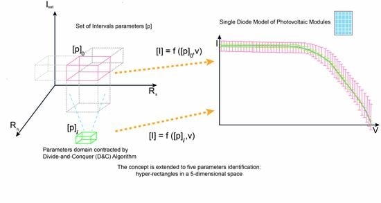
In the next section, on the basis of such conclusions, the proposed IA parametric identification method is shown: it starts from a large rectangle in the parameters domain exemplified by the gray rectangle in the qualitative example of Figure 3, and contracts it in order to bound as much as possible the experimental points, which are marked in blue in Figure 3, in the I-V domain.

4. Parametric Identification by the IA-Based Divide-and-Conquer ($D\&C$) Algorithm

In this paper, the identification of all the five parameters in (5) is considered. As a consequence, the rectangles shown in Figure 3 have to be considered hyper-rectangles in a 5-dimensional space. Iteration by iteration, the initial intervals $\left[P\right]$ are contracted in order to contract the $\left[I\right]$ around the experimental data. The iterations end when a termination condition fixed by the user is fulfilled. The divide-and-conquer ($D\&C$) algorithm is an algorithm design paradigm for discrete and combinatorial optimization problems. The algorithm starts evaluating the largest candidate set of parameters assigned by the user, which is named ${\left[P\right]}_0$ in Figure 4. If the $\left[I\right]$ bounds include the experimental I-V samples $(I_{exp},V_{exp})$, then all the five parameters intervals of ${\left[P\right]}_0$ are halved, so that $2^5$ sub-intervals are generated.

For each of the $2^5$ sub-intervals the I-V boundary is calculated by using IA. If the experimental points $(I_{exp},V_{exp})$ are not included in the boundaries, the corresponding subset is marked as infeasible and it is not partitioned into smaller subsets anymore. On the contrary, the subset is partitioned by halving again the intervals it is made of and these ones are analyzed at the next iteration level. Thus, the algorithm continues with the next dividing level until a termination condition fixed by the user is fulfilled.

In summary, the proposed $D\&C$ algorithm consists of the following main elements appearing in Figure 4.

Dividing Level (i): it is identified by the sub-index i. At each level, the parameters’ intervals sets that fulfill the feasibility condition are halved, so that $2^5$ new sub-intervals are generated. Thus, in case all the intervals are feasible, at the dividing level i a number $2^{5x\mathit{i}}$ is generated and its feasibility has to be tested. Each interval in the subset takes a new sub-index $\mathit{j}$, so that a particular set of parameters is called ${\left[P\right]}_{i,j}$. For instance, at the branching level $i=1$, each element in the interval ${\left[P\right]}_0=[\left[R_s\right];\left[R_h\right];\left[I_{sat}\right];\left[B\right];\left[I_{ph}\right]]$ is halved, and all the $2^{5x1}=32$ combinations of these sub-intervals, which are called: ${\left[P\right]}_{1,1}...{\left[P\right]}_{1,32}$, have to be tested through the feasibility condition.

Feasibility condition: at the i-th branching level, the subset of intervals ${\left[P\right]}_{i,j}$ is substituted in (5) for each voltage value $V_{exp}$ of the experimental data set. A current interval $\left[I\right]$ results at each voltage value and it is verified that the all the $N_p$ experimental points fall within the calculated intervals:

$$I_{exp,n_p}\in \left[I(\left[P\right],V_{n_p})\right],forall{n}_p=1,\dots ,N_p$$

(6)

Parameters’ sub-intervals ${\left[P\right]}_{i,j}$ that do not fulfill the feasibility condition are not divided anymore and are not transferred to the next algorithm iteration.

It is worth noting that the infeasibility of these sub-intervals is guaranteed by the use of IA. Indeed, IA properties recalled in Section 3 ensure that the co-domain $\left[I\right]=f\left(\right[P],V)$ evaluated over a set of parameters $\left[P\right]$ is an overestimation of the true range spanned by the current I for that domain $\left[P\right]$. As a consequence of the overestimation, if the range $\left[I\right]$ does not fulfill the feasibility condition, namely, does not include all the experimental I-V samples, then it is guaranteed to be infeasible. The same guarantee would be achieved by classical methods, e.g., Monte Carlo, only at a very high cost, even tending towards an infinite computational cost, thanks to the trials in the Monte Carlo approach. This represents a relevant advantage of the proposed IA based approach.

Termination condition: Feasible intervals ${\left[P\right]}_{i,j}$ falling below a minimum width, which is wid${\left[P\right]}_{i,j}$, fixed by the user, are not divided further. Thus:

$$wid{\left[P\right]}_{i,j}\le \Delta D·mid{\left[P\right]}_{i,j}$$

(7)

where $mid{\left[P\right]}_{i,j}$ represents the midpoint of ${\left[P\right]}_{i,j}$. When the termination condition imposes that no more feasible intervals have to be partitioned further, then the union of the feasible intervals achieved by the algorithm represents the final result. The proposed IA-based $D\&C$ algorithm is presented in Algorithm 1.

Algorithm 1: IA-based $D\&C$ algorithm.

5. Identification of the Parameters $R_s$, $R_h$ and $I_{sat}$ through the IA-based $D\&C$ Method

The identification of the SDM parameters almost consists of identifying $R_s$, $R_h$ and $I_{sat}$. Indeed, the $I_{ph}$ parameter is assumed as equal to the short-circuit current [2], whose value is experimentally measured. On the other hand, once having measured the cells’ temperature and by assuming that the number of series connected cells in the module is known, the value of the parameter B is fixed if, as it is quite common in literature, (see [8,34,35]), n assumes a value between 1 and 2. Typical values are below 1.5, but the search range has been extended up to 2 in order to account for more extreme cases documented in literature [36]. It has to be kept in mind that the range is subjected to the contraction due to the IA based approach proposed in this paper. Thus, a smaller upper limit would not affect the final result of the identification process, but its rate of convergence. With those assumptions, the identification process limited to the three parameters $R_s$, $R_h$ and $I_{sat}$ is of practical interest and allows one to demonstrate the performance of the proposed $D\&C$ algorithm on a reduced scale case. The algorithm in this case is tested by using I-V samples that are obtained by using the parameters in Table 2 in the SDM (5). Samples are calculated at a fixed voltage step $0.1V$, so that the $N_p=222$ I-V samples shown in Figure 5 are considered.

The $D\&C$ algorithm has run on the following search space: $\left[R_s\right]=[0.1,1]\Omega ;\left[R_h\right]=[1,1000]\Omega ;\left[I_{sat}\right]=[1e^{-8},1e^{-12}]A$. The nominal values for B and $I_{ph}$ given in Table 2 have been also used. $\Delta D=1.5\%$ has been used for settling the termination condition.

The algorithm has created the number of dividing levels shown in

Table 3. Number of feasible intervals, percentage of infeasible intervals and volume of the subsets at each dividing level for the example using noiseless data.

Dividing Level	Number of Feasible Intervals	% of Infeasible Intervals	Subsets Volume
1	4	50.00%	1.2361 $\times {10}^{-6}$
2	9	71.88%	1.5452 $\times {10}^{-7}$
3	3	95.83%	1.9315 $\times {10}^{-8}$
4	4	83.00%	2.4143 $\times {10}^{-9}$
5	5	84.38%	3.0179 $\times {10}^{-10}$
6	4	90.00%	3.7724 $\times {10}^{-11}$
7	6	81.25%	4.7155 $\times {10}^{-12}$
8	4	91.60%	5.8944 $\times {10}^{-13}$
9	5	84.38%	7.3680 $\times {10}^{-14}$
10	2	95.00%	9.2100 $\times {10}^{-15}$

. The third column of Table 3 reveals the effectiveness of the proposed IA approach. Indeed, as pointed out before, the main advantage of applying IA to the feasibility condition is the immediate and guaranteed classification of the infeasible sets of the search space. It is evident that, for this example, just at the first dividing level, 50% of the search space is immediately classified as infeasible. The same result would require a number of Monte Carlo trials instead of four IA based computations. The fourth column of Table 3 gives a measure of the volume of each subset at the corresponding dividing level. The solution is reached at the tenth dividing level, at which two sets of interval solutions have been identified. The union of those two intervals is shown in

Table 4. Interval solution by $D\&C$ algorithm in the example using noiseless data.

Parameters	Initial Intervals	Union of Intervals in the Space of Solutions
$\left[R_s\right]$	[0.1,1] $\Omega$	[0.179189,0.180156] $\Omega$
$\left[R_h\right]$	[1,1000] $\Omega$	[150.265,151.24] $\Omega$
$\left[I_{sat}\right]$	[1 $\times {10}^{-12}$,1 $\times {10}^{-8}$] A	[5.28291 $\times {10}^{-10}$,5.4782 $\times {10}^{-10}$] A

. It reveals that the interval set solution contains the values of parameters $R_s$, $R_h$ and $I_{sat}$ used to generate the I-V samples. This is the expected result, so that the convergence property of the $D\&C$ algorithm is confirmed. A personal computer (PC) equipped with a Corei7-3632QM processor @ 2.20 GHz, four cores and 8 GB of RAM memory is used. The executable file, produced by starting from the C++ source, was run on a PC. With this software and hardware, the algorithm reaches the solution in 1.02 s after 360 iterations. Figure 5 puts into evidence that all the I-V samples fall inside of interval current $\left[I\right]$ determined by the IA based method.

This first test has been done by identifying the parameters by using I-V samples obtained through the same model, the SDM, adopted for the identification thereof. In this way, the process has not been affected by inaccuracies of the SDM in fitting experimental data and by inaccuracies and noise over I-V measurements. These effects will be more evident in the next sections wherein experimental I-V data are used.

6. $D\&C$ IA-Based Approach Applied to Experimental Data

Experimental I-V data are commonly affected by noise due to, e.g., sensor quality and the data acquisition system’s resolution. The low voltage region usually is the most critical because it requires a high resolution of the current sensor. Similarly, although not so seriously as in the previous case, at low current the voltage sensor has to show a significant resolution. In the presence of noise, such critical aspects become more and more significant. Therefore, the proposed $D\&C$ method has been made more robust in order to cope with noisy experimental data. Firstly, the decision on whether the experimental value is within or outside the IA determined $\left[I\right]$ interval is taken by account for a suitably small noise band around the experimental value. Additionally, the feasibility condition is relaxed by considering that an interval set of parameters is feasible if a number, but not all, of the experimental data fulfill the condition (6). The effects of these two additional conditions are analyzed in detail in the following subsections.

6.1. Relaxation of the Inclusion Property: First Approach

In Figure 6, the blue circles, which are the experimental data, are surrounded by blue bars representing a noise band, named $\left[I_{exp}\right]$. The red bars bound the interval of the current $\left[I\right]$, which is computed by IA on a given interval parameters set. Thus, the inclusion property is reformulated by considering that the experimental value (blue dots) is included in the interval range (red interval) if the intersection between the red range and the blue range of that experimental point is not empty. The larger the noise or the uncertainty, e.g., related to the sensors used, affecting the experimental data, the wider the band $\left[I_{exp}\right]$ and the higher the probability that the intersection between $\left[I_{exp}\right]$ and $\left[I\right]$ is not empty, and thus that the corresponding set of parameters is feasible.

6.2. Relaxation of the Inclusion Property: Second Approach

In (8), the feasible condition that relaxes the (6) by marking as feasible a parameter set for which $N_p^{-}<N_p$ experimental points fall within the I-V boundaries is formalized. This approach allows one to restrict the application of the feasibility condition to some regions of the I-V curve wherein the major information content is concentrated. For instance, the experimental I-V samples that are more affected by measurement noise can be excluded, or the feasibility condition can be limited to a region including the MPP, to the short circuit and to the open circuit conditions.

$$\left[I_{exp,n_p}\right]\in \left[I(\left[P\right],V_{})\right],for{n}_p=1,\dots ,N_p^{-}$$

(8)

6.3. $D\&C$ Parametric Identification by Using Noisy Experimental Data

Figure 7 shows an experimental set of I-V data referring to a 140W PV Yingli solar module that have been acquired at an irradiance equal to 849 W/m² and at a temperature equal to $336.15$ K: they have been measured by using a low cost system described in detail in [37], which has the drawback of providing a high number of data in the low current range and a low density of measurements at low voltages. The I-V curve is obtained by the capacitor charging method, which takes an acquisition time of 0.05 s. The experimental setup is described in detail in [37]: the PV module output is made available in the laboratory through a 10 m long cable. Thus, the acquired I-V curve also takes into account the parasitic resistance of the cables, which is 60 m$\Omega$. Figure 7 shows that the module under test has suffered degradation, due to 3.5 years of long operation.

6.3.1. Identifying $\left[R_s\right]$, $\left[R_h\right]$,$\left[I_{sat}\right]$, $\left[B\right]$ and $\left[I_{ph}\right]$

The parameter $N_p^{-}$ in (8) has been settled to 216, so that $90\%$ of experimental points have been taken into account for the feasibility condition. Thus, 10% of points are excluded, regardless of their position in the I-V curve, but the short-circuit current $I_{sc}$ and the open circuit voltage $V_{oc}$ have been always included in the 90%, so that the feasibility condition for this example has been formalized as in (9):

$$\begin{array}{c}\hfill \left[I_{exp,n_p}\right]\in \left[I(\left[P\right],V_{n_p})\right],for{n}_p=1,\dots ,N_p^{-}\\ \hfill [I_{exp,1}]\in \left[I(\left[P\right],V_1)\right]\\ \hfill [I_{exp,N_p}]\in \left[I(\left[P\right],V_{N_p})\right]\end{array}$$

(9)

The current samples at low voltage show noise close to $1\%$ of their values; thus, the parameter appearing in the termination condition $\Delta D$ is fixed at 10%.

Table 5. Number of feasible intervals, percentage of infeasible intervals and volume of the subsets at each dividing level for the example using experimental I-V data.

Dividing Level	Number of Feasible Intervals	% of Infeasible Intervals	Subsets Volume
1	14	56.25%	8.3219 $\times {10}^{-4}$
2	148	66.96%	2.6006 $\times {10}^{-5}$
3	1089	77.00%	8.1269 $\times {10}^{-7}$
4	6326	81.85%	2.5396 $\times {10}^{-8}$
5	5817	97.13%	7.9364 $\times {10}^{-10}$

collects the number of feasible intervals at each division level. Additionally, in this example, from the third column of Table 5, it comes out that the IA approach guarantees the infeasibility of 56.25% of the initial search space at the first dividing level. Indeed, of the initial $2^5=32$ subsets, 18 are guaranteed to be infeasible by a direct computation of $\left[I\right]$ through IA. These results reveal that the IA-based $D\&C$ proposed algorithm finds the solution at the dividing level 5, in which there are 5817 interval sets that have been classified feasible. The algorithm spent 11.68 min to run 242,496 iterations. It is worth noting that these numbers are significantly higher than those ones achieved in the example presented in Section 5. This is due to the presence of noise, affecting the experimental samples and not the simulated samples of the previous case, and it is also a consequence of the chosen value of the termination threshold, which is now fixed at $\Delta D=10\%$, and thus greater than $\Delta D=1.5\%$ used in the previous example. The union of the feasible intervals sets achieved at the last dividing level is given in the third column of

Table 6. Interval solution by the $D\&C$ algorithm at the final dividing level in the example using experimental I-V data.

Parameters	Initial Intervals	Union of Feasible Intervals
$\left[R_s\right]$	$[0.1,1]\Omega$	$[0.26875,0.60625]\Omega$
$\left[R_h\right]$	$[300,800]\Omega$	$[300,800]\Omega$
$\left[I_{sat}\right]$	[1 $\times {10}^{-8}$,1 $\times {10}^{-4}$]A	[3.12569 $\times {10}^{-5}$,7.81272 $\times {10}^{-5}$]A
$\left[B\right]$	[0.7,1.5]	[1.375,1.5]
$\left[I_{ph}\right]$	[7.0271,7.7669]A	[7.397,7.42012]A

. The contraction of the intervals with respect to the initial search space has been also shown.

In Figure 8, red bars give the current intervals calculated by substituting the interval solution of Table 6 in (5) and using IA. At least 90% of experimental data, those in blue marks, fall inside the interval current $\left[I\right]$. Nevertheless, although a significant contraction of the search space has been achieved by the $D\&C$ method (see Table 6), the interval solution (red bars) still gives a large range around the experimental points. As it will be shown in the next subsection, an improved identification accuracy is achieved by analyzing the feasible sub-intervals achieved by the $D\&C$ method at a given dividing level.

The identified intervals achieved and shown in Table 6 can be used to identify, in turn, some additional SDM parameters. For instance, the interval $B=[1.375,1.5]$ can be used to identify the corresponding interval of the diode ideality factor n, again by using IA. Indeed, it results that:

$$n=\frac{B·q}{N_s·k·T}=\frac{[1.375,1.5]·1.60217662·{10}^{-19}}{36·1.38064852·{10}^{-23}·336.15}=[1.31854,1.43841]$$

(10)

Additionally, the uncertainty of the devices used in the temperature measurement system can account for: a LM35 installed on rear side of the PV module, a non-inverting amplifier and a 10 bit ADC. In this case, the uncertainty affecting the temperature measurement is equal to 0.8%. Thus, it results that:

$$n=\frac{[1.375,1.5]·1.60217662·{10}^{-19}}{36·1.38064852·{10}^{-23}·[333.461,338.839]}=[1.30808,1.45001]$$

(11)

Both the intervals achieved for n are in a suitable range for this parameter. The same procedure might be applied by identifying further physical parameters underlying the set of five shown in Table 6.

6.3.2. Analysis of the Feasible Sub-Intervals

In the previous example, the final solution obtained through the IA based algorithm was determined as the union of all the feasible sets of intervals achieved at the final dividing level. Each sub-interval can be examined in more detail by calculating the current obtained, at each voltage value of the experimental samples, through SDM (5) using the midpoints $mid\left[P\right]$ of the interval of each parameter. This calculated current is called $I\left(mid\right[P],V)$. Then, the root-mean-square error (RMSE) of the identified current with respect to the experimental $I_{exp}$ is calculated. In (12), the RSME formula is shown, which takes into account the number of samples $N_p$. The sub-interval giving the I-V curve having the minimum value of the RMSE is considered as the best. This analysis has been applied to the feasible sub-intervals in Table 5, so that 5817 set of intervals have been evaluated. The second column of

Table 7. $mid{\left[P\right]}_{best}$ and the corresponding interval solution with the smallest RMSE value.

Parameters	$\mathbf{mid}{\left[\mathit{P}\right]}_{5,\mathbf{best}}$	Best Interval Solution
$R_s$	0.4797 $\Omega$	[0.4656, 0.4938] $\Omega$
$R_h$	792.1875 $\Omega$	[784.3750, 800] $\Omega$
$I_{sat}$	4.5318 $\times {10}^{-5}$ A	[4.3756 $\times {10}^{-5}$, 4.6880 $\times {10}^{-5}$] A
B	1.4625	[1.4500, 1.4750]
$I_{ph}$	7.4086 A	[7.3970, 7.4201] A

shows the $mid{\left[P\right]}_{5,best}$ found in the 5817 sets in the space solutions, which correspond to the interval set ${\left[P\right]}_{5,4350}$. The fit of the I-V curve generated using $mid{\left[P\right]}_{5,best}$ is presented in Figure 9. The minimum RMSE value achieved is 0.0659.

$$RMSE=\sqrt{\frac{\sum _{i=1}^{N_p}{(I_{exp}-I(mid\left[P\right],V))}^2}{N_p}}$$

(12)

In Figure 10, the I-V curve generated by SDM using the best sub-interval, which is shown in the third column of Table 7, is depicted: the contraction of the initial interval set with respect to the Figure 8 is evident.

6.3.3. Identifying $\left[R_s\right]$, $\left[R_h\right]$,$\left[I_{sat}\right]$, $\left[B\right]$ and $\left[I_{ph}\right]$ by the $D\&C$ Algorithm with Emphasis Around the MPP

The experimental points of the I-V curve across its MPP are of primary importance for the parametric identification of the SDM, and they might be excluded by the procedure described above. In this example, the experimental data around the MPP and limited to the range $[80\%,100\%]$ of the power at the MPP, which is $P_{\mathrm{MPP}}$, are considered. The left and right extremes are shown in Figure 9, Figure 10 and Figure 11 in black and gray, and are named $0.8P_{\mathrm{MPP}}^{-}$ and $0.8P_{\mathrm{MPP}}^{+}$. Those power values correspond to the samples called $N_p^{0.8P_{\mathrm{MPP}}^{-}}$ and $N_p^{0.8P_{\mathrm{MPP}}^{+}}$, respectively. All the experimental points in this range have been included in the feasibility condition (13). The tolerance around experimental data $I_{exp}$ and the termination condition $\Delta D$ have been fixed at $1\%$ and $10\%$ respectively.

Relaxed feasibility condition with constraints of $I_{sc}$ and $V_{oc}$ and less data.

$$\begin{array}{c}\hfill \left[I_{exp,n_p}\right]\in \left[I(\left[P\right],V_{n_p})\right],for{n}_p=N_p^{0.8P_{\mathrm{MPP}}^{-}},\dots ,N_p^{0.8P_{\mathrm{MPP}}^{+}}\\ \hfill [I_{exp,1}]\in \left[I(\left[P\right],V_1)\right]\\ \hfill [I_{exp,N_p}]\in \left[I(\left[P\right],V_{N_p})\right]\end{array}$$

(13)

The results of $D\&C$ algorithm are shown in

Table 8. Number of feasible intervals, percentage of infeasible intervals and volume of the subsets at each dividing level for the example using a reduced set of experimental data.

Dividing Level	Number of Feasible Intervals	% of Infeasible Intervals	Subsets Volume
1	14	56.25%	8.3219 $\times {10}^{-4}$
2	144	67.86%	2.6006 $\times {10}^{-5}$
3	1032	77.60%	8.1269 $\times {10}^{-7}$
4	5495	83.36%	2.5396 $\times {10}^{-8}$
5	2890	98.36%	7.9364 $\times {10}^{-10}$

. Again, in this example, at the first dividing level, IA classifies as infeasible 18 subsets over 32, just by a direct IA based computation of the current interval $\left[I\right]$. The solution is reached at the dividing level 5, in which the space of solutions contains 2890 sub-intervals. In this case the algorithms needs 213,952 iterations; thus, the computation time and memory are reduced with respect to the previous examples. The number of feasible sub-intervals in the final dividing level is reduced by $51.4\%$ and the number of iterations is reduced by $11.7\%$. The union of the final sub-intervals is given in

Table 9. Interval solution by the $D\&C$ algorithm in the example using a reduced set of experimental data.

Parameters	Initial Intervals	Union of Feasible Intervals
$\left[R_s\right]$	[0.1,1]$\Omega$	[0.325,0.55]$\Omega$
$\left[R_h\right]$	[300,800]$\Omega$	[300,800]$\Omega$
$\left[I_{sat}\right]$	[1 $\times {10}^{-8}$,1 $\times {10}^{-4}$]A	[3.12569 $\times {10}^{-5}$,7.81272 $\times {10}^{-5}$]A
$\left[B\right]$	[0.7,1.5]	[1.375,1.5]
$\left[I_{ph}\right]$	[7.0271,7.7669]A	[7.397,7.42012]A

, and it reveals the contraction with respect to the initial search space. The set of intervals is similar to the one obtained by using all the experimental values; $R_s$ is the only one showing an improved contraction.

In Figure 12, the red bars correspond to SDM evaluated by IA for the solution presented in Table 9. As in the previous case, large ranges result from the union of the feasible sub-intervals at the final dividing level where the algorithm terminated. The analysis of the RMSEs for all the feasible sub-intervals at the division level 5 gives a narrower range. The best sub-interval is the same as that achieved in the previous example, and is shown in Table 7 and Figure 10. The best sub-interval set is ${\left[P\right]}_{5,2272}$, and the minimum RMSE value is 0.0776.

7. Discussion of the Results

Some aspects concerning the results presented in the previous examples deserve further comments. The first one concerns the way in which the initial interval set of parameters, and thus the search space, is chosen. The proposed IA-based $D\&C$ algorithm was run on an initial interval set ${\left[P\right]}_0$ that was generally very large, just in order to test the convergence and contraction capabilities of the approach. In the first example, which referred to the identification of the values of three parameters only and used I-V data generated by the same model used for the identification thereof, a large initial interval set was used. The initial intervals for the two resistances were set to include typical values; thus, they were in the order of magnitude of hundreds of m$\Omega$ and hundreds of $\Omega$ for series and parallel resistances respectively. Such initial intervals might also include values corresponding to a degraded PV module. The initial interval of $I_{ph}$ has been chosen across the short-circuit current value $I_{sc}$.

By using the I-V experimental measurements around the MPP, the $I_{ph}$ is settled at values that are close to the MPP current $I_{mpp}$; thus, an initial interval across $I_{mpp}$ is used. The initial ranges of B and $I_{sat}$ have been determined by keeping account of some physical relationships. The parameter B depends on temperature T and n: it has been assumed that T has been measured with a known accuracy and that the ideality factor, as can be deduced from the literature referring to silicon cells, assumes values ranging from $n=1$ up to $n=2$. The larger the uncertainty affecting the measure of the temperature, the wider the initial interval ${\left[B\right]}_0$. As for $I_{sat}$, it has been assumed that, for new PV modules, it assumes values of the order of $nA$ while $\mu A$ is used for aged modules. The ${\left[I_{sat}\right]}_0$ width affects the convergence features of the approach significantly. The proposed examples show the convergence capability of the $D\&C$ algorithm even using a ${\left[I_{sat}\right]}_0$ that is four orders of magnitude and has n ranging up to 2, instead of stopping at 1.3, as can be deduced by reading some papers; e.g., [35]. However, a better trade-off between accuracy and computation time should be reached by having a more accurate estimation of the initial range of the parameters.

The second aspect deserving further comments concerns the selection of the value $\Delta D$ involved in the termination condition (7), because it affects the accuracy of the result and the computation time required by the algorithm. In the case a low noise level affecting the I-V samples, a tiny termination condition does not affect the computation time significantly, as in the first example. Indeed, any relaxation of the inclusion property is required and a small number of feasible intervals at each dividing level is obtained. In the case of I-V experimental data exhibiting a significant noise level, a trade-off between accuracy and computation time needs to be achieved. Some relaxation of the inclusion property and a higher value of $\Delta D$ help to achieve the convergence. It is worth noting that the number of feasible subsets obtained at the end of each algorithm run depends on both the ability of the SDM to fit the experimental curve and on the chosen $\Delta D$ value. The additional step using the RMSE calculation discussed in some examples presented in Section 5 and Section 6 helps to improve the accuracy of the IA solution.

The third remark concerns the size of interval current $\left[I\right]$, as it is shown in Figure 8, Figure 10 and Figure 12. In the SDM solution shown in Figure 8 and Table 6, the relative width of the interval parameters’ solution ($wi{d}_m\left[P\right]$), is calculated by $\frac{wid[\underline{x},\overline{x}]}{\mathit{mid}[\underline{x},\overline{x}]}$. The results are $wi{d}_m\left[R_s\right]=0.7714$, $wi{d}_m\left[R_h\right]=0.9091$, $wi{d}_m\left[I_{sat}\right]=0.8570$, $wi{d}_m\left[B\right]=0.0870$ and $wi{d}_m\left[I_{ph}\right]=0.0031$. Figure 12 shows the I-V curve boundaries corresponding to the same interval solution, by neglecting the range of $\left[R_s\right]$. In this case, the relative width is 0.5143; thus, the important effect of the $\left[R_s\right]$ interval on $\left[I\right]$ becomes evident. By using the RMSE calculation in Table 7, the relative interval sizes are reduced to the following values: $wi{d}_m\left[R_s\right]=0.0588$, $wi{d}_m\left[R_h\right]=0.0197$, $wi{d}_m\left[I_{sat}\right]=0.0689$, $wi{d}_m\left[B\right]=0.0171$ and $wi{d}_m\left[I_{ph}\right]=0.0031$. The significant effect of this contraction on the range $\left[I\right]$ is evident by looking at Figure 10. The contraction is close to one order of magnitude for all the parameters, but not for $\left[I_{ph}\right]$. Figure 2 shows that $\left[I_{sat}\right]$ and $\left[B\right]$ have significant effects on the $\left[I\right]$ width. Figure 13 shows that the true range of $\left[I\right]$ is overestimated because of the use of IA, especially at high voltage. The overestimation is evident by comparing the IA results with those ones obtained by means of a Monte Carlo run over 2000 random trials. The corresponding I-V curves are shown in black color, which have been generated by randomly choosing sets of parameters in the ranges shown in Table 7. It is worth noting that the Monte Carlo method giving a narrower range with respect to the IA method does not mean that the former result is more accurate than the latter one. Indeed, only if both of them are taken into account, exact information about the true range spanned by I at the different voltages is obtained. Indeed, the Monte Carlo range would approach the true one by running an infinite number of trials; otherwise it gives an underestimation of the true range of I. The IA overestimation is reduced by reducing the width of the interval parameters [33]. The true range is placed in the middle, bounded by the Monte Carlo range, which is an underestimation of the true range, and the IA range, which is an overestimation of the true range.

An additional advantage of the proposed IA-based $D\&C$ algorithm can be put into evidence by referring to the results shown in

Table 10. Performance comparison of Matlab Fit APP tool using the intervals of Table 6.

Feature	Using the Initial Intervals	Using the Union of Feasible Intervals	Improvement
Number of iterations	67	13	80%
Number of function evaluations	408	84	79%
Step Size	0.0707	5.2217 $\times {10}^{-6}$	Four orders of magnitude

. The Matlab Fit APP tool has been used to identify the five parameters of SDM. It minimizes the root mean square error between the experimental I-V data and I-V curve obtained through the SDM with the identified values of the parameters. The trust-region method has been selected, the function tolerance value has been settled at 1e-5 and the maximum number of iterations has been fixed at 400. In the second column the results achieved by this tool are given. The initial interval of the parameters has been set equal to the initial interval used in the proposed IA-based $D\&C$ algorithm; thus, the one given in the second column of Table 6. The third column of Table 10 shows the result when the initial search space used in Matlab Fit APP is the union of the feasible intervals obtained by the the proposed IA-based $D\&C$ algorithm; thus, the one in the third column of Table 6. It is evident that the proposed IA based approach has contracted the initial search space towards the solution in an effective way, so that the Matlab Fit APP converges to the identified set by a number of iterations and function evaluations that is 80% lower than the one required if the search is started from the wider search space used by the IA $D\&C$ method. Moreover, the step size is reduced by four orders of magnitude, so that a higher accuracy in the parameter identification is achieved. This result reveals that the feasible intervals obtained by the proposed IA-based $D\&C$ algorithm are reliable guess solutions for gradient based minimization methods. The cascade of the methods thus allows one to improve the convergence and the accuracy of the result. The RMSE value obtained by Matlab Fit APP is equal to 0.0587, which is close to the one obtained by the proposed analysis procedure of the feasible sub-intervals ($mid{\left[P\right]}_{5,best}$ shown in Table 7), which is 0.0659. The $D\&C$ IA-based method uses a simple partitioning of the intervals and feasibility test, and thus, any gradient or minimization method, also guaranteeing the infeasibility of the discarded intervals.

As a further comment concerning the implementation of the IA-based $D\&C$ algorithm, it has to be evidenced that it might profit significantly from a parallel implementation of the IA operations. Indeed, in any IA operation, the computations of the lower bound and of the upper bound of the result can be done in parallel, because these two computations are independent. Moreover, the computation tree derived from the proposed $D\&C$ method is also prone to a parallel computation. Consequently, the proposed algorithm, which has been already developed in C++ by means of a suitable library including all the IA operations, can be implemented in embedded devices including multi-core processors or field programmable gate arrays (FPGAs).

8. Conclusions

In this paper an interval-arithmetic-based approach has been applied for identifying the five parameters of the single-diode model of crystalline silicon photovoltaic modules. The divide-and-conquer computational paradigm has been used to contract an initial interval set of parameters, that is, the search space, towards an interval parameters set of a suitably small width. The proposed method generates feasible and infeasible intervals by successive divisions of the initial search space. Each interval is evaluated by a feasible condition through interval arithmetic: this key operation allows one to discard infeasible portions of the search space with a single operation, without involving any iterative procedure or any minimization algorithm. Moreover, interval arithmetic guarantees the infeasibility of the discarded sets, meaning that no combinations of parameters in those sets give a current vs. voltage curve that is more close to the experimental samples than the curves obtained by the feasible sets. After discarding the infeasible intervals, the proposed method reduces the widths of the feasible ones until they fall below a threshold fixed by the user through the termination condition. The performance of the proposed algorithm has been tested on three examples, including simulated data and experimental data, the latter affected by measurement noise. The analysis of the case using experimental measurements has evidenced the need for a further computation step that profits from the interval contraction capabilities of interval arithmetic, allowing one to refine the final interval solution. In addition to the main feature of parametric identification, the proposed algorithm gives some information that should be useful in the detection of aging, malfunctioning and faults of the photovoltaic generator. Indeed, the final result of the application of the method gives an indication about the sensitivity of the model with respect to the five parameters appearing in it. Moreover, the ranges provided by the method and including the experimental current vs. voltage samples give a mask for linking the variation of the module performance to the variation of its parameters. Thanks to the interval arithmetic inclusion properties, current values acquired in the same operating conditions and falling outside the interval ranges would reveal variations of the parameters that are outside the corresponding ranges. For instance, by applying this on-site evaluation to the series resistance, the aging of the module exceeding a fixed threshold can be detected. The offline computation of the interval boundaries in the current vs. voltage plane and their uploading on a low cost processor would allow a straightforward and on-site verification of the violation of these boundaries with negligible computation effort.