Abstract
With the rapid increase in photovoltaic energy production, there is a need for smart condition monitoring systems ensuring maximum throughput. Complex methods such as drone inspections are costly and labor intensive; hence, condition monitoring by utilizing sensor data is attractive. In order to recognize meaningful patterns from the sensor data, there is a need for expressive machine learning models. However, supervised machine learning, e.g., regression models, suffer from the cumbersome process of annotating data. By utilizing a recent state-of-the-art semi-supervised machine learning based on probabilistic modeling, we were able to perform condition monitoring in a photovoltaic system with high accuracy and only a small fraction of annotated data. The modeling approach utilizes all the unsupervised data by jointly learning a low-dimensional feature representation and a classification model in an end-to-end fashion. By analysis of the feature representation, new internal condition monitoring states can be detected, proving a practical way of updating the model for better monitoring. We present (i) an analysis that compares the proposed model to corresponding purely supervised approaches, (ii) a study on the semi-supervised capabilities of the model, and (iii) an experiment in which we simulated a real-life condition monitoring system.
1. Introduction
With an ever increasing growth in photovoltaic (PV) energy production, the sheer size of individual power plants is growing at a rapid pace [1]. Building and operating such PV plants has become a viable business in many countries. High PV energy production and maximized yield are fundamental for a profit margin. The challenge is not solely detecting an anomaly in the PV power plant, but also optimizing the operation and maintenance costs once detected [2]. Condition monitoring plays a crucial role, since it is key to identifying the specific system state to ascertain its impact on energy production and ensure minimal maintenance costs; e.g., panel cleaning and replacements, and circuit or diode checks [3]. Another challenge is the size of the PV plants. Minimally, the performance of the strings or arrays needs to be monitored. In a MW range there will be hundreds of PV performance computational streams to monitor in real time or periodically [2].
Many PV plant conditions can result in decreased yield. Amongst the conditions are (i) weather patterns, (ii) PV panel aging, (iii) evolving faults, e.g., diode failure or glass breakage, and (iv) faulty installation of the PV panels [4]. It is quite simple to detect anomalies in energy production; however, it is more complex to find the sources of the anomalies accurately. Furthermore, the cause may be a result of a chain of events for which the causality is very much non-trivial.
Several alternatives for better condition monitoring exist, many of which include quite costly add-ons; e.g., increased amount/accuracy of sensors and infrared inspection [5]. Another complementary approach is traditional statistical analysis of the data [6], but this is resource intensive. A less expensive alternative is a data-driven approach in which supervised machine learning models parameterized by, for example, neural networks, learn from the vast amount of incoming sensor data. These machine learning models have proven efficient in terms of noise resiliency and for finding non-linear correlations within condition monitoring for wind energy [7,8] and PV plants [9,10,11]. However, there is an inherent problem in assumptions made when applying highly expressive neural networks to the problem of condition monitoring, since they are mostly formulated in a supervised setting. This means that we generally expect a large dataset containing condition-data with adhering labels. Therefore, in order to get started, one must (i) predefine all potential non-overlapping conditions that may happen in a PV plant, (ii) have a vast distribution of annotated data-points for each condition, and (iii) expect no anomalies from the already defined problem. It is quite clear that executing (i) will introduce a constraint on how specific we can be in defining a condition, since many have a tendency to overlap. Task (ii) is also limiting since the data of a PV plant is not directly interpretable by a human. Therefore, one needs to engage in a costly annotation of data-points in order to train the relatively data-hungry neural networks. Finally, (iii) is posing a limit of supervised neural networks, since they are normally not modeled with an uncertainty, resulting in a risk of an overly confident estimate of a severe anomaly [12].
Before proposing a solution to the above, it is important to specify how PV plant condition-data can be defined. In this research the conditions are expressed by the output of sensors, monitoring the PV array current, voltage, in-plane irradiance, external temperature, PV module temperature, and wind speed. The sensor inputs are recorded with a specific temporal resolution. The hypothesis is that, in cohesion, all of these sensor inputs will have unique patterns representing a PV plant condition. We propose a state-of-the-art semi-supervised probabilistic machine learning framework that can capture the unique patterns and cluster them according to their respective similarities. Furthermore, as part of the framework, a supervised classifier, taught with a pre-defined annotation process, categorizes each of these clusters. The probabilistic framework thus models the joint distribution of the condition data and the PV plant state. This should be contrasted to traditional supervised approaches that model the state given the condition data. The big advantage of the model is that it can capture condition data anomalies while also classifying known conditions. In addition to this, the number of annotated data-points needed is very low.
The machine learning framework works by learning a distribution over the PV power plant conditions, and thereby correlates new data points with the learned distribution. In recent years there have been several notable contributions within probabilistic semi-supervised learning methods. Amongst them are [13,14], which utilize the variational auto-encoder framework (VAE) [15,16] for a Bayesian approach to modeling the joint probability between the data and labels. In this paper we utilize the skip deep generative model (SDGM) from [14].
The paper is structured such that we give a background to PV condition monitoring, supervised machine learning for fault detection, and the SDGM. Next we introduce the experimental setup followed by results. We show that SDGM can indeed be used as a machine learning model for condition monitoring, and performs significantly better than its supervised counterparts, even in a fully supervised setting. Finally, we simulate a real-life condition monitoring setup where PV plant conditions are introduced sequentially. In these experiments we show how SDGM is able to detect anomalies, and that retraining the system improves condition monitoring performance.
2. Detection and Identification of PV Power Loss and Failures trough Classification Methods
2.1. PV Failures and Factors Causing Power Loss
There exists a number of external factors that can cause power loss in a PV system, in addition to PV specific degradation modes [4]. These can be roughly categorized into three groups. The first group covers optical losses and degradation, such as soiling, snow, or shading affecting the module surface [17], and discoloration of the encapsulant [4]. These optical power loss factors can be relatively easily detected through visual inspection; however, this is not always feasible for large or hard to reach PV installations. Moreover, detecting them from production measurements can be difficult, since their associated failure patterns in the power measurements are irregular, depending on the size and relative position of the soiling, shading, etc. Detecting such failures is important, since some of them can be remedied relatively easy, through cleaning of the PV panels.
A second category of factors causing power loss in a PV system, is the degradation of the electrical circuit of the PV module. In the most severe cases, these are represented by open-circuit and short-circuit faults within the PV array and associated cabling [4]. But there can also be partial degradation, due to moisture ingress and corrosion of the electrical pathways [18], causing an increased series resistance of the PV array [19]. Such faults are generally difficult to detect through visual inspection, and require thermal IR imaging or electroluminescence to detect. However, they cause more predictable patterns in the production measurements, such as voltage drops proportional to the increase in series resistance. Such failures can cause localized heating and hot-spots, posing a risk of arcing and fire.
The third category corresponds to degradation of the solar cells, which in turn can occur due to a number of stress factors, such as: (i) thermo-mechanical stress, causing solar cell cracks, associated with increased series resistance, shunting, and localized heating [4,19]; (ii) voltage stress, causing potential-induced degradation, primarily associated with a decrease in the cells’ shunt resistance, but also corrosion and delamination in the case of some thin film technologies [20]; (iii) diurnal and seasonal variations affecting solar cells with metastable performance behavior, such as certain thin film technologies [21]. Degradation modes in this category are more difficult to detect, and the associated failure patterns in production measurements are more complex. Nonetheless, identifying such failures in their incipient phase is of utmost importance, since they are symptoms of more serious, system-wide problems, such as bad system design, installation practice, or module quality, which should be resolved while the modules and PV system are still in warranty.
The types of power loss factors and degradation modes that can affect PV systems are varied and difficult to formalize. And, only a few of them may affect a PV system within its lifetime, depending mainly on the solar cell technology, panel design and quality, environmental and operational conditions, and installation and maintenance practices.
2.2. Failure Detection through Supervised Classification
Two of the main prerequisites for implementing supervised classification in a condition monitoring system, are: (i) the a priori knowledge of the fault types/classes that will occur/need to be detected in the PV system; and (ii) representative measurement datasets for each of the fault classes, necessary for training the classification model. Once these perquisites are met, and appropriately monitored, production variables are chosen as input, and classifiers are trained for each fault class. Once trained, each classifier will operate continuously, monitoring the production variables, and will be able to discern if the system is in normal operation, or if a specific fault class has occurred.
Many types of supervised classification algorithms exist; e.g., support vector machines (SVM) [22], random forest (RF) [23], and multilabel logistic regression (MLR). These are all very expressive models; however, with the rise of deep learning [24], we have seen a multitude of improvements from models that can capture highly non-linear correlations in the data. The improvements mainly concern areas such as image classification [25] and automatic speech recognition [26]. However, the more expressive models also gain traction within renewable energy; e.g., for condition monitoring in wind turbines [8] and as forecasting models for solar irradiance [27]. Defining the deep neural network is not a simple task, due to the vast number of choices that need to be taken in regard to type of architecture, depth, regularization, and much more.
The main challenge in implementing a supervised classification algorithm for detecting faults in a PV system is obtaining the necessary PV production measurement datasets characterizing the different fault classes. Since there are no standardized fault classes and representative datasets, faults of different types and severity can occur throughout the 25+ year expected lifetime of the PV system.
2.3. Proposed Failure Detection through Semi-Supervised Classification
A possible solution is to combine a supervised classification method with a data clustering method that is able to detect anomalous patterns in the monitored PV production data. Next, on-site inspection of the event/fault by maintenance personnel, can help identify the type or class of this event/fault. The associated production measurements can then be used to retrain a supervised classifier for the detected event/fault class, such that future instances of the event/fault will be automatically detected and identified by the condition monitoring system, which continuously learns new fault classes as it operates (Figure 1).
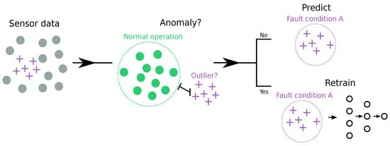
Figure 1.
A visualization of the condition monitoring system. The sensor data is propagated through the machine learning framework, and the model detects whether the data point is an outlier. If it is an outlier, the sensor data must be manually inspected, and the machine learning framework retrained. If the incoming sensor data is not an outlier, the framework will predict the state of the condition. If the fault state is detected, as a fault, maintenance will be scheduled accordingly.
We propose to solve the problem for semi-supervised condition monitoring by teaching a feature representation z of the PV condition data x as a continuous conditional probability density function, , and the classification task of the PV state y as a discrete conditional probability density function, . In order to teach both models jointly from both labeled and unlabeled data, the two models must be defined such that they share parameters. By applying Bayes theorem we can formulate the problem by:
where we assume the latent variable feature representation z and state labels y are to be a priori statistically independent, . In a scenario with complex input distributions, e.g., sensor input from a PV power plant, the posterior , becomes intractable. Therefore, we formulate the problem such that we learn an approximation, , to the posterior through variational inference [28]. SDGM is an example of this probabilistic framework which enables the use of stochastic gradient ascent methods for optimizing the parameters of the generative model, , and the variational approximation, . and denote the parameters of the generative model and the variational approximation (also denoted inference model) respectively. Both are constructed from deep neural networks (cf. Figure 2). We learn the model parameters by jointly maximizing the objective for labeled data and for unlabeled data :
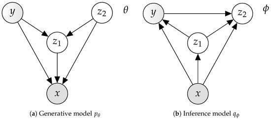
Figure 2.
The graphical model of the SDGM for semi-supervised learning [14]. The model is defined by two continuous latent variables, and , a partially observed discrete latent variable y, and a fully observed input x. (a) The generative model and (b) the inference model, also known as the variational approximation. Each union of incoming edges to a node defines a densely connected deep neural network.
SDGM defines two continuous latent variables, , and the discrete partially observed latent variable y [14]. The continuous distributions for the latent variables z are defined as Gaussian distributions and the discrete distribution y is a Categorical distribution. For the labeled data we optimize the parameters, with respect to a lower bound on the evidence (ELBO):
with
Since the labeled ELBO does not include the classification error, we add the categorical cross-entropy loss
where is a constant scaling term defined as a hyper-parameter. Similarly to the labeled loss, we define the unlabeled loss as the unlabeled ELBO:
where
In this paper we restrict the experiments to only use densely connected neural networks, but simple extensions to the model include recurrent neural networks and convolutional neural networks that have proven efficient in modeling temporal and spatial information within condition monitoring [8,27]. Besides being among the state-of-the-art within semi-supervised image classification, SDGM posses another intriguing property for condition monitoring, differentiating it from other semi-supervised approaches. Since we are optimizing the ELBO, we can use this as an anomaly measure. Thus, if the value of the ELBO for a specific data-point is far below the value of the unlabeled ELBO, that was evaluated during optimization, we can define the data-point as an anomaly.
3. Experimental Application and Tests
In order to validate whether the proposed SDGM can be utilized for condition monitoring, we have recorded a dataset of the sensor data from a small-scale PV plant. During the timespan of the recording, we witnessed 10 different categories that we used as labels. In order to benchmark the machine learning framework, we have defined two comparable supervised machine learning models.
3.1. Field Test Setup and Dataset
To evaluate the progressive learning and fault detection capabilities of the proposed condition monitoring system, we performed measurements and tests on a 0.9 kWp roof-mounted PV string (eight multicrystalline silicon modules). The PV string was connected to a 6 kWp Danfoss TLX Pro string inverter that was continuously monitoring the string current (I), voltage (V), plane-of-array irradiance (G), external temperature (TExt), module temperature (TMod), and windspeed (W), with a one minute sampling time. Since the test PV system is normally not affected by any faults, we created seven power loss events/fault classes by applying different types of shading on the panels, and by connecting different power resistors on series with the PV string, to emulate series resistance type faults. In addition, we also recorded PV production for when the PV system was covered by snow, for a clear sky, and for a cloudy sky day. The ten conditions/fault classes are outlined in Table 1, and will be used as class labels for testing the classifiers in the next sections. Another important step in designing a classification model is choosing appropriate input variables. Minimally, PV array current and voltage are monitored in a PV system, and we denote this case as the simple monitoring case. Additional monitoring input variables can be the solar irradiance, module temperature, external temperature, and wind speed. These are less commonly monitored in small PV installations, due to the additional costs of the sensors; however, in larger PV plants, these are usually monitored by accurate weather stations. We will denote the case including the ambient conditions as input variables, the complex monitoring case.

Table 1.
An overview of the PV system dataset used for this research. The dataset comprises 10 categories from approximately 15,000 data samples of a varied representation.
The categories are skewed in accordance to the weather pattern during the two months; e.g., there is a majority of data points for which there was snow (cf. Table 1). For each learned model, we ran a 5-fold Monte Carlo cross-validation with a random split of for training and for testing. The labeled samples are either sampled uniformly or progressively for each PV system state category.
3.2. Machine Learning Setup
In order to evaluate the proposed machine learning framework, we first define a solid baseline for comparison. Since the SDGM is parameterized by neural networks, we construct a supervised neural network for classification with similar parameterization to . Furthermore, we also define a simple linear classification model, in order to conclude whether the added complexity from the neural networks is needed for modeling this dataset. The supervised deep neural network for classification is denoted multi-layer perceptron (MLP), and the linear model is referred to as multi-label regression (MLR).
(i) In the first experiment we benchmark SDGM against MLP and MLR in a fully supervised setting; thus, all labels for the entire dataset are given during training. The aim of this experiment is to see whether MLP performs significantly better than MLR and whether SDGM performs approximately equivalently to MLP. We perform this experiment on both the simple and complex monitoring case. (ii) Next, we investigate the semi-supervised performance of the SDGM. In order to do this, we simulate a scenario where only a fraction of data in the PV sensor dataset is given. Since MLP and MLR are supervised models, they are only able to learn from this fraction of labeled data, whereas SDGM can utilize the unlabeled fraction also. The fraction of labeled data is randomly sampled uniformly across categories, such that there is an even representation of each category in the labeled dataset. (iii) Finally, we simulate a real-life PV plant condition monitoring system, in which we assume that each condition is introduced to the power plant sequentially (cf. Figure 1). First, we initialize the dataset with only one labeled data-point from each category, in order to introduce the minimal amount of categorical knowledge in the classifier. Next we introduce 500 labeled samples from the first category in Table 1 and optimize MLP and SDGM. Then we could estimate the ELBO in Equation (7) for the data-points of the categories that are included during training and the ones that are not. We also estimate the accuracy of each classifier in SDGM and the MLP. We expected that the estimate of the ELBO would be significantly lower for the categories that are not included in the dataset as opposed to the ELBO for the categories that are included. This indicates an anomaly. Then, we progressively include another category from Table 1 and perform the same analysis until we have evaluated 6 categories.
The SDGM (For details on experimental implementation and code refer to [14] and the corresponding Github repository.) consists of 2 densely connected deep neural neural networks with parameters in the generative model and 3 densely connected deep neural networks with parameters in the inference model. The neural networks in both the SDGM and MLP contains 2 hidden layers with 50 units in each. We use the ReLU [29] activation function as a non-linearity and ADAM [13] for optimizing the parameters. For the MLP we use a dropout [30] rate of and for the MLR we use L2 regularization. Model training is stopped upon saturation of the validation error. The constant is defined as in [14]. During optimization of the SDGM we utilize the warm-up introduced in [31,32].
4. Results
We performed three experiments, introduced above. In the first experiment we benchmarked the SDGM against the MLP and MLR in a fully-supervised setting. Next we evaluated the semi-supervised power of the SDGM. Finally, we simulated a real-life condition monitoring system.
4.1. Supervised Condition Monitoring Accuracy
Table 2 presents the baseline results of MLR, MLP, and SDGM in a fully supervised learning setup. By utilizing more sensor attributes (complex versus simple), the performance increases well over 10% across all models. This proves that the additional sensor inputs (G, TExt, TMod, and W) are very useful for condition monitoring. When comparing the non-linear MLP to the linear MLR we also achieve a significant improvement in performance, indicating that the input data is not linearly separable, and that the added complexity of the neural networks is worthwhile.
Table 2.
Fully supervised baselines of MLR, MLP, and SDGM with the simple sensor input, {I, V}, and the complex input, {I, V, G, TExt, TMod, and W}.
The most surprising finding was that the SDGM performs significantly better than MLP. We believe that this is due to the fact that SDGM also learns a latent clustering of the data that is correlated with the PV state.
Thereby, the model can discriminate between the labels and the cluster representations, meaning that it can put less emphasis on labeled information that does not seem to correlate with the distribution. Hence, if a small fraction of faulty labels exist in the training dataset, SDGM is able to ignore this information and thereby achieve better generalization towards the validation dataset.
Figure 3 shows how the wrongly classified examples from the MLR and MLP are quite similar. The highest misclassification rate lies between cloudy and snowy weather, {C, S}. Other misclassification rates mainly lie between {RS8, PS50}, {N, RS4}, {RS8, IV}, and {N, RS4}. When we compare the results of MLR and MLP to the SDGM (cf. Figure 4a) we can read from the confusion matrix that the SDGM manages to learn the difference between cloudy and snowy, {C, S}. Furthermore the remainder of the most prominent misclassification rates are significantly decreased. In order to analyze what is learned in the latent variables of SDGM, we plot the first two principal components from a principal component analysis (PCA) (cf. Figure 4b). The visualization of the latent space shows clear discrimination between categories. Furthermore, we can also see that the data lies on manifolds resembling the movement of the sun.
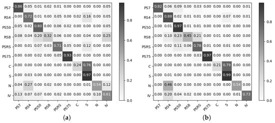
Figure 3.
Normalized confusion matrices for (a) MLR and (b) MLP trained on the fully labeled complex dataset. The x-axis denotes the predicted labels and the y-axis the true labels.
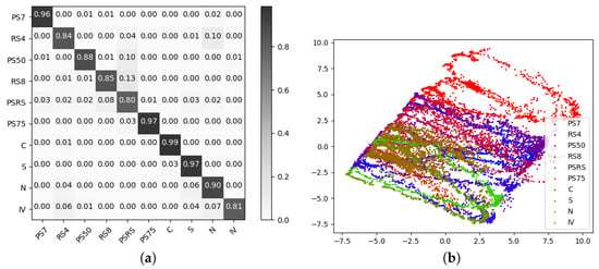
Figure 4.
(a) Normalized confusion matrices for SDGM trained on the fully labeled complex dataset. (b) PCA (principal components 1 and 2) on the latent space.
4.2. Semi-Supervised Condition Monitoring Accuracy
In order to evaluate the semi-supervised performance of SDGM, we define eight datasets with different fractions of labeled data that are randomly subsampled across the categories in Table 1 for each of the trained models, {100, 300, …, 1500}. Figure 5 shows SDGM’s significant increase in performance by utilizing the information in the unlabeled data. For the simple dataset, with {I, V} as input, we see that the supervised models, MLR and MLP, achieve an accuracy of 35%–45% by learning from 100 labeled data-points, whereas the SDGM achieves 55%–60%. As expected, the relative improvement from using SDGM stays significant when introducing more labels. Similarly to the supervised analysis above, all models achieve a significant improvement when adding more sensor inputs, {I, V, G, TExt, TMod, W}. When comparing the results of the semi-supervised SDGM with the supervised SDGM, we see that the models trained on 1500 labeled data points actually exceed the performance of the fully-supervised model, compared to . Again, the reason for this may be that with fewer labeled examples, SDGM put a larger emphasis on the unlabeled data, and thereby it was not as prone to faulty annotations. In Figure 6 we visualize the latent representations by PCA for the SDGM trained with 100 labeled data-points on the simple and complex input. It is clear that the model trained on the complex is better at discriminating between the categories than the model trained on the simple input. Furthermore, when comparing Figure 4b with Figure 6b we see clear indications that the increase in labels results in better discrimination between condition states.
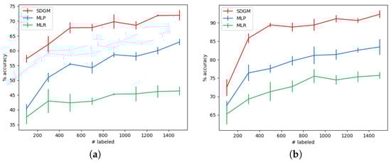
Figure 5.
Comparison between the supervised MLP, MLR, and the semi-supervised SDGM trained on an increasing amount of randomly sampled and evenly distributed labeled data points. For each number of labeled data points, we trained 10 different models, since a large variance between the quality of the subsampled labeled data points may have existed. (a) The accuracy with one standard deviation for models trained on the simple input distribution {I, V}, and (b) the accuracy for models trained on the complex input distribution, {I, V, G, TExt, TMod, W}.
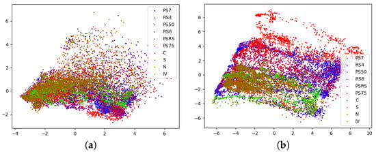
Figure 6.
PCA (principal component 1 and 2) visualization of the latent space for SDGMs trained a dataset with only 100 labeled samples. (a) The latent space for a model trained on the simple dataset, {I, V} and (b) for {I, V, G, TExt, TMod, W} as input.
4.3. Adding PV Conditions Progressively
In a PV system it is highly unlikely that a dataset will consist of an evenly distributed labeled dataset from all categories. To test whether the SDGM is able to perform anomaly detection on the data, we set up an experiment where we began by learning a model on 500 randomly sampled labeled data points and only one labeled data point for each of the remaining categories. Then, we progressively taught new models with a dataset to which we added 500 labels for the next category. We continued this procedure until the 6th category.
Figure 7a presents the results of a SDGM and MLP taught up to six categories. As expected, the accuracy for all categories increases when more categories are added to the dataset. Again, it is clear that the SDGM is able to utilize the information from the unlabeled examples and the very sparse information from the other categories to significantly outperform the MLP. In Figure 7b, we visualize the level of certainty and ELBO (cf. Equation (7)), and can easily discriminate the categories included during training from the categories that are not included. So for a model trained on only {PS7} data, it is easy to detect {RS4, PS50, RS8, PSRS, PS75, C, S, N, IV} conditions as anomalous, and for a model trained on {PS7,RS4} it is easy to detect {PS50, RS8, PSRS, PS75, C, S, N, IV} as anomalous. In order to state whether a PV plant condition is an anomaly, the operator needs to define a threshold value. In this experiment a suitable threshold could be that PV plant conditions with an ELBO below nats is considered an anomaly. Upon realization of an anomaly, the PV plant operator will initiate a brief annotation process and retrain the SDGM framework, so that the new states are within the known operational condition.
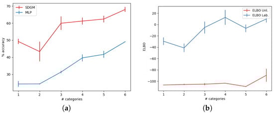
Figure 7.
SDGMs and MLPs were trained with datasets from which we randomly subsampled a single data-point from each category and then progressively added 500 randomly labeled data points for each category, and we trained a new MLP and SDGM for each progression. (a) The accuracy of the classifiers for the SDGM and MLP. (b) The ELBO for the data categories included during training (ELBO Lab.) The data categories that are not included during training (ELBO Unl.). The categories that were progressively added followed the order of Table 1; i.e., first {PS7}, and next {PS7, RS4}, until reaching {PS7, RS4, PS50, RS8, PSRS, PS75}.
Figure 8 presents the classification errors for the MLP and SDGM when only taught on 100 labeled data points. Since the SDGM is able to utilize the information of the unlabeled data points it is also able to classify much better across PV plant categories.
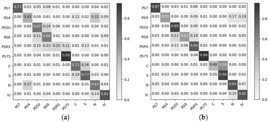
Figure 8.
Normalized confusion matrices for (a) MLP and (b) SDGM trained on 100 randomly sampled and evenly distributed labeled data points. The x-axis shows the predicted labels, and the y-axis the true labels.
5. Conclusions
In this research we have proposed a novel machine learning framework to perform PV condition monitoring that simultaneously learns classification and anomaly detection models. We have shown that the proposed semi-supervised framework is able to improve over a fully supervised framework when given a full set of labeled data points (fully supervised learning) and when only given a fraction of labeled data points (semi-supervised learning). We have also shown that the framework is able to identify previously unknown fault types by performing anomaly detection, and how it can be easily retrained in order to capture these PV states. This approach can significantly improve the throughput of energy production and lower the maintenance cost of PV power plants. We have shown that the approach is easy to train on a rather simple dataset and that it is easily interpretable by evaluating the classification results, the latent representations, and the lower bound of the marginal log-likelihood.
The main limitation of this research lies in the dataset used. Due to the representation and the amount of samples, it does not resemble the vast amount of data one could acquire from a large-scale PV power plant. However, deep neural networks have a tendency to improve when introduced to more data, meaning that we can hypothesize that the results would only improve. In this regard, an interesting direction for future research would be to investigate the possibility for transfer learning between PV power plant configurations, so that one could seamlessly deploy the framework taught on one PV plant to another.
Author Contributions
Conceptualization, L.M. and S.S.; methodology, L.M., O.W., S.S., and D.S; software, L.M.; validation, L.M. and S.S.; formal analysis, L.M. and S.S.; investigation, L.M. and S.S.; resources, L.M., S.S., and D.S.; data curation, S.S. and D.S.; writing—original draft preparation, S.S. and L.M.; writing—review and editing, S.S., D.S., O.W., and L.M.; visualization, L.M.; supervision, D.S. and O.W.; project administration, D.S. and O.W.; funding acquisition, O.W. and D.S. All authors have read and agreed to the published version of the manuscript.
Funding
This research was funded by Danish National Advanced Technology Foundation, grant number HTF 102-2013-3.
Acknowledgments
The research was supported by the NVIDIA Corporation with the donation of TITAN X GPUs.
Conflicts of Interest
The authors declare no conflicts of interest.
References
- IEA PVPS. Trends 2017 in Phtovoltaic Applications—Survey Report of Selected IEA Countries between 1992 and 2016; International Energy Agency: Paris, France, 2018.
- Mütter, G.; Krametz, T.; Steirer, P. Experiences with a performance package for multi-MW PV plants based on computations on top of monitoring. In Proceedings of the 31st European Photovoltaic Solar Energy Conference and Exhibition WIP, Hamburg, Germany, 14–18 September 2015; pp. 1675–1678. [Google Scholar]
- Woyte, A.; Richter, M.; Moser, D.; Reich, N.; Green, M.; Mau, S.; Beyer, H.G. Analytical Monitoring of Grid-Connected Photovoltaic Systems; International Energy Agency: Paris, France, 2014.
- Köntges, M.; Kurtz, S.; Packard, C.; Jahn, U.; Berger, K.A.; Kato, K.; Friesen, T.; Liu, H.; Van Iseghem, M. Review of Failures of Photovoltaic Modules; International Energy Agency: Paris, France, 2014.
- Buerhop-Lutz, C.; Scheuerpflug, H.; Pickel, T.; Camus, C.; Hauch, J.; Brabec, C. IR-Imaging a Tracked PV-Plant Using an Unmanned Aerial Vehicle. In Proceedings of the 32nd European Photovoltaic Solar Energy Conference and Exhibition WIP, 2016, Munich, Germany, 20–24 June 2016; pp. 2016–2020. [Google Scholar]
- Vergura, S.; Acciani, G.; Amoruso, V.; Patrono, G.E.; Vacca, F. Descriptive and Inferential Statistics for Supervising and Monitoring the Operation of PV Plants. IEEE Trans. Ind. Electron. 2009, 56, 4456–4464. [Google Scholar] [CrossRef]
- Bach-Andersen, M. A Diagnostic and Predictive Framework for Wind Turbine Drive Train Monitoring. Ph.D. Thesis, Technical University of Denmark, Lyngby, Denmark, 2017. [Google Scholar]
- Bach-Andersen, M.; Rømer-Odgaard, B.; Winther, O. Deep learning for automated drivetrain fault detection. Wind Energy 2017, 21, 29–41. [Google Scholar] [CrossRef]
- Silvestre, S.; Chouder, A.; Karatepe, E. Automatic fault detection in grid connected PV systems. Sol. Energy 2013, 94, 119–127. [Google Scholar] [CrossRef]
- Jiang, L.L.; Maskell, D.L. Automatic fault detection and diagnosis for photovoltaic systems using combined artificial neural network and analytical based methods. In Proceedings of the IEEE International Joint Conference on Neural Networks, Killarney, Ireland, 12–17 July 2015. [Google Scholar]
- Ali, M.H.; Rabhi, A.; El Hajjaji, A.; Tina, G.M. Real Time Fault Detection in Photovoltaic Systems. Procedia Energy 2017, 111, 914–923. [Google Scholar] [CrossRef]
- Gal, Y. Uncertainty in Deep Learning. Ph.D. Thesis, University of Cambridge, Cambridge, UK, 2016. [Google Scholar]
- Kingma, D.P.; Rezende, D.J.; Mohamed, S.; Welling, M. Semi-Supervised Learning with Deep Generative Models. In Proceedings of the International Conference on Machine Learning, Beijing, China, 21–26 June 2014; pp. 3581–3589. [Google Scholar]
- Maaløe, L.; Sønderby, C.K.; Sønderby, S.K.; Winther, O. Auxiliary Deep Generative Models. In Proceedings of the International Conference of Machine Learning, New York, NY, USA, 19–24 June 2016. [Google Scholar]
- Kingma, D.P.; Welling, M. Auto-Encoding Variational Bayes. In Proceedings of the International Conference on Learning Representations, Scottsdale, AZ, USA, 2–4 May 2013. [Google Scholar]
- Rezende, D.J.; Mohamed, S.; Wierstra, D. Stochastic Backpropagation and Approximate Inference in Deep Generative Models. arXiv 2014, arXiv:1401.4082. [Google Scholar]
- Laukamp, H.; Schoen, T.; Ruoss, D. Reliability Study of Grid Connected PV Systems, Field Experience and Recommended Design Practice; International Energy Agency: Paris, France, 2002.
- Yang, B.B.; Sorensen, N.R.; Burton, P.D.; Taylor, J.M.; Kilgo, A.C.; Robinson, D.G.; Granata, J.E. Reliability model development for photovoltaic connector lifetime prediction capabilities. In Proceedings of the 39th IEEE Photovoltaic Specialists Conference (PVSC), Tampa, FL, USA, 16–21 June 2013; pp. 139–144. [Google Scholar]
- King, D.L.; Quintana, M.A.; Kratochvil, J.A.; Ellibee, D.E.; Hansen, B.R. Photovoltaic module performance and durability following long-term field exposure. Prog. Photovolt. Res. Appl. 2000, 8, 241–256. [Google Scholar] [CrossRef]
- Luo, W.; Khoo, Y.S.; Hacke, P.; Naumann, V.; Lausch, D.; Harvey, S.P.; Singh, J.P.; Chai, J.; Wang, Y.; Aberle, A.G.; et al. Potential-induced degradation in photovoltaic modules: A critical review. Energy Environ. Sci. 2017, 10, 43–68. [Google Scholar] [CrossRef]
- Silverman, T.; Jahn, U.; Friesen, G.; Pravettoni, M.; Apolloni, M.; Louwen, A.; Schweiger, M.; Belluardo, G. Characterisation of Performance of Thin-film Photovoltaic Technologies; International Energy Agency: Paris, France, 2014.
- Cortes, C.; Vapnik, V. Support-Vector Networks. Mach. Learn. 1995, 20, 273–297. [Google Scholar] [CrossRef]
- Breiman, L. Random Forests. Mach. Learn. 2001, 45, 5–32. [Google Scholar] [CrossRef]
- Hinton, G.E.; Osindero, S.; Teh, Y.W. A Fast Learning Algorithm for Deep Belief Nets. Neural Comput. 2006, 18, 1527–1554. [Google Scholar] [CrossRef] [PubMed]
- He, K.; Zhang, X.; Ren, S.; Sun, J. Deep Residual Learning for Image Recognition. In Proceedings of the IEEE Conference on Computer Vision and Pattern Recognition, Las Vegas, NV, USA, 27–30 June 2016; pp. 770–778. [Google Scholar]
- Xiong, W.; Wu, L.; Alleva, F.; Droppo, J.; Huang, X.; Stolcke, A. The Microsoft 2017 Conversational Speech Recognition System. arXiv 2017, arXiv:1708.06073. [Google Scholar]
- Alzahrani, A.; Shamsi, P.; Dagli, C.; Ferdowsi, M. Solar Irradiance Forecasting Using Deep Neural Networks. Procedia Comput. Sci. 2017, 114, 304–313. [Google Scholar] [CrossRef]
- Jordan, M.I.; Ghahramani, Z.; Jaakkola, T.S.; Saul, L.K. An Introduction to Variational Methods for Graphical Models. Mach. Learn. 1999, 37, 183–233. [Google Scholar] [CrossRef]
- Glorot, X.; Bordes, A.; Bengio, Y. Deep Sparse Rectifier Neural Networks. In Proceedings of the 14th International Conference on Artificial Intelligence and Statistics (AISTATS), Ft. Lauderdale, FL, USA, 11–13 April 2011; Volume 15, pp. 315–323. [Google Scholar]
- Srivastava, N.; Hinton, G.; Krizhevsky, A.; Sutskever, I.; Salakhutdinov, R. Dropout: A Simple Way to Prevent Neural Networks from Overfitting. JMLR 2014, 15, 1929–1958. [Google Scholar]
- Sønderby, C.K.; Raiko, T.; Maaløe, L.; Sønderby, S.K.; Winther, O. Ladder Variational Autoencoders. In Advances in Neural Information Processing Systems; Neural Information Processing Systems (NIPS): Barcelona, Spain, 2016. [Google Scholar]
- Bowman, S.; Vilnis, L.; Vinyals, O.; Dai, A.; Jozefowicz, R.; Bengio, S. Generating sentences from a continuous space. arXiv 2015, arXiv:1511.06349. [Google Scholar]


© 2020 by the authors. Licensee MDPI, Basel, Switzerland. This article is an open access article distributed under the terms and conditions of the Creative Commons Attribution (CC BY) license (http://creativecommons.org/licenses/by/4.0/).