Abstract
This work focuses on the demand response (DR) participation using the energy storage system (ESS). A probabilistic Gaussian mixture model based on market operating results Monte, Carlo Simulation (MCS), is required to respond to an urgent DR signal. However, there is considerable uncertainty in DR forecasting, which occasionally fails to predict DR events. Because this failure is attributable to the intermittency of the DR signals, a non-cooperative game model that is useful for decision-making on DR participation is proposed. The game is conducted with each player holding a surplus of energy but incomplete information. Consequently, each player can share unused electricity during DR events, engaging in indirect energy trading (IET) under a non-cooperative game framework. The results of the game, the Nash equilibrium (N.E.), are verified using a case study with relevant analytical data from the campus of Gwangju Institute of Science and Technology (GIST) in Korea. The results of the case study show that IET is useful in mitigating the uncertainty of the DR program.
1. Introduction
Advancements in technology are always accompanied by changes, and the energy arena is no exception. These changes, such as an increase in distributed energy resources and renewable energy (RE), introduced the concepts of transactive energy (TE) for effecting electricity democratization [1]. According to the GridWise Architecture Council, TE is “a set of economic and control mechanisms that allow the dynamic balance of supply and demand across the entire electrical infrastructure using value as a key operational parameter” [2]. Likewise, the use of RE is rapidly spreading in Korea following the Renewable Energy 3020 Plan, which was announced by the Ministry of Trade, Industry & Energy in 2017. The goal of this plan is to increase the capacity of RE by 20% of the total generation capacity by 2030; the current status of RE capacity in Korea is about 178 GW [3]. Under these conditions, flexible resources, such as Energy Storage Systems (ESS), high ramping rate generators, and demand response (DR) have become essential for handling the intermittency of RE generation. Among these candidates, DR can be deployed to handle this flexibility efficiently [4].
Generally, DR is divided into two parts: the first involves the use of tariffs and the other is operated as an incentive-based system [5]. Korea operates a DR market using some incentives, and this study will deal primarily with incentive-based DRs. Furthermore, there are two sub-programs in the DR market and they are operated for different purposes: the first is meant to reduce the system marginal price by replacing peak generation, and is referred to as economic DR. The other, reliability DR, is designed to secure reliable capacity for entire power systems, meaning that reliability DR can substitute other generators as needed. However, the operation performance of the DR market in Korea remains unsatisfactory. By way of illustration, in 2018, seven DR dispatch signals were ignored, even though they satisfied the dispatch conditions. This uncertainty makes potential participants reluctant to join the market, and current market operation results show less activity than that observed last year [6]. However, global trends leave little doubt that DR is an indispensable resource. Accordingly, there are studies providing precedents for the use of DR in Korea [7,8,9]. Kang and Lee [7] studied the capacity for participation in the DR program in Korea. In [8,9] there are suggestions regarding the ESS algorithm needed for participation in the economic DR. However, this approach is very limited, and the effects of participation are minimal. Thus, this suggestion is unlikely to appeal to potential participants.
The Guide to the expression of Uncertainty in Measurement (GUM) is one of the well-established approaches toward evaluating the uncertainty problem [10]. However, GUM approach has some critical limitations [11] and as a way of overcoming the limitations of GUM, Monte Carlo Simulation (MCS) is being considered as an advanced approach toward evaluating uncertainty [11,12,13,14]. For this reason, MCS is used to handle uncertainty in the electric field [15,16,17]. In [15,16], MCS is used to deal with the uncertainty problem in DR, and Shi [17] estimated uncertainty from household energy data with MCS.
As rational decision-makers agree that game theory is a powerful mechanism for coping with complex interactions [18], this theory is a fitting approach to solving the many decision-making problems encountered in the power industry [19]. In fact, game theory is already used for decision-making processes in various fields in the power system. Prior work [20] suggests that game theory consists of two segments, the cooperative game and the non-cooperative game. A cooperative game is mainly used by groups of players to achieve shared joint objectives, and this game is applied in the power system to model allocations of shared energy [21,22,23]. In non-cooperative games, each self-regulating player makes its own determination and this may serve the interests of each player suitably [20]. This advantage supports the implementation of the non-cooperative game to model the interactions of the prosumer’s behavior [24,25,26,27,28]. Reference [24] introduces a non-cooperative game that shows the ESS scheduling pattern resulting from Nash equilibrium (N.E.). In addition, [25] uses the game to suggest purchasing strategies from a retailer’s perspective. Finally, other studies show that the non-cooperative game constitutes an effective method of handling DR decision-making [26,27,28]. These results support the notion that the non-cooperative game could provide a satisfactory way of responding to problems with DR.
An ESS algorithm for participating in economic DR is suggested in [8], but the results show that there is no economic rationale for participating in the DR with ESSs because of the low-level benefits of economic DR. Thus, this work proposes suggestions on ways to use the ESS to participate in a reliability DR program that ensures greater benefits exhibiting uncertainties. Furthermore, a non-cooperative game allowing the DR participants to use indirect energy trading (IET) to share surplus electricity and to decrease the uncertainties in the current DR conditions in Korea is described. As a result, the DR participation of ESS is profitable through IET.
2. Demand Response Participation of Buildings with ESS in South Korea
2.1. Demand Response in Korea
As mentioned earlier, the DR market is operated using two sub-programs. Unlike economic DR, which is operated on the principle of day-ahead bidding, reliability DR is operated on more of a real-time basis. For example, in reliability DR, the Korea Power Exchange (KPX) dispatches a signal to all participants one hour ahead of the projected need, and the participants must respond to the signal. Thus, predicting the dispatching of a signal is difficult and, because this uncertainty is directly related to the participants’ anticipated benefits, the uncertainty causes them to hesitate using their ESS to cooperate with the DR program [8]. Likewise, participants can receive two types of payments if they participate in the reliability DR. The first is based on actual performance, and the other is proportional to the register capacities, and is a type of capacity payment. However, if they fail to respond to a signal on more than three occasions in a year, they cannot receive any payment even when they respond to the other signals. This response is calculated relative to the historical load data, which is called the Customer’s Base Line (CBL).
2.2. Operational Strategy of ESS for DR Participation
For the prediction of DR operations, we must consider two elements: the day on which the DR event occurs, and the time at which the DR signal is dispatched. There are a set of conditions that trigger a reliability DR dispatch, and they are related to demand level and supply reserve, so it is possible to predict the day of an upcoming dispatch to a certain extent by considering the demand and supply. Thus, we assume a prediction rate for the day of a DR event. Meanwhile, we can sample the DR event time by developing a probabilistic model based on performance results. Table 1 shows the operational results in the Korean DR market, which is used to construct a model that forecasts the time of the DR event.

Table 1.
Reliability DR operation results in Korea, in 12-month increments.
As shown in Table 1, the number of samples are insufficient, so we use Bayesian estimation to infer the probabilistic model because it is reliable even with small samples [29]. The estimated model is a Gaussian Mixture Model (GMM), and the appearance of the probability distribution function calculated from Equation (1) is as shown in Figure 1.
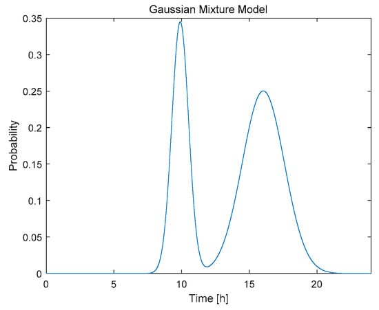
Figure 1.
Probabilistic model of reliability demand response (DR) prediction.
The performance in a reliability DR call is calculated using the CBL, which is estimated by considering the average load profile during the five days before the signal is dispatched. Thus, the ESS operational strategy involves consideration of the time of the DR event, as well as the customer’s pattern of load in the CBL.
Consequently, two ESS scheduling patterns are suggested, and they are developed using the probabilistic model and the CBL. The ESS specifications are assumed to be 500 kWh capacity, with an 80% depth of discharge 80%; meaning that the lower limit of the ESS state of charge (SOC) is 10% and the upper limit is 90%. Moreover, the wear-out cost is not considered here. The first pattern is the probabilistic method; according to the probabilistic model (Figure 1); 10 a.m. has the highest potential for the occurrence of a morning DR event, and 4 p.m. exhibits the highest potential for an event in the evening. As the probability of a DR event is relatively higher, if the ESS is expected to discharge relatively less power during this time, the remainder of the capacity can be used for DR situations. For example, if the ESS discharge pattern for a CBL is 40 kWh at 10 a.m., as shown in Figure 2, about 360 kWh can be used in a DR event, while approximately 350 kWh is available at 9 a.m. Thus, the high probability of a DR event leads to low discharge patterns for the CBL; Figure 2 confirms that the results reflect these expectations. Another method involves shutting down the ESS for five days before the CBL, it means there is no variation in ESS scheduling during five days. This strategy necessitates a participant to refrain from operating the ESS when a DR event day is predicted. In this case, the opportunity cost should be considered because the participants would have derived benefits from arbitrage if they had not chosen this method.
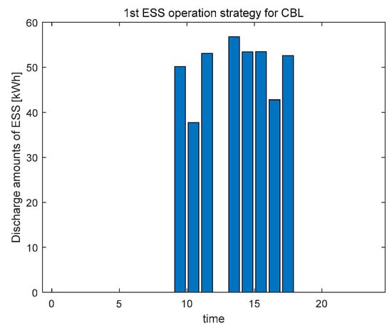
Figure 2.
Energy Storage Systems (ESS) scheduling with Gaussian Mixture Model (GMM).
2.3. Uncertainty of DR Participation from Monte Carlo Simulation (MCS)
The operational results (Table 1) allow us to assume that every DR event will last for approximately two hours, and in the last year of the dataset, DR events were recorded for about 30 h. Therefore, we set a scenario wherein a DR signal occurred on 15 days during the year (Scenario 2 in Table 2). Furthermore, according to KPX (ISO in Korea), there is an upper bound on the total time of DR events equaling 60 h per year. Thus, a high frequency of DR signals would correspond to 25 days during a year, and a low frequency of DR signals would correspond to five days in a year, as seen for years 1–3 in Table 1. Furthermore, the DR event could be forecasted as mentioned earlier, so the ability to predict the day of a DR event is assumed to exhibit 50% accuracy. With these parameters, we generated 500,000 prediction profiles for each scenario, and the parameters are as shown in Table 2.
Table 2.
Monte Carlo Simulation (MCS) parameters.
The uncertainty of DR participation means that DR participants will not receive payments because of non-compliance with the DR signal from failure of DR prediction. This is where the concept of marginal capacity, which is similar to the marginal generator in economic dispatch, is introduced. It means if the DR register capacity of ESS is slightly increased over the marginal capacity, the uncertainties of DR participation are dramatically increased. Figure 3 show this concept well.
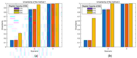
Figure 3.
Uncertainty by ESS register capacity of each method: (a) method 1, (b) method 2.
Method 1 is showed in Figure 3a, and if participants participate in DR at 50% or 51% of their ESS capacity, the uncertainty is similar. However, if they choose the marginal capacity, which is 52% in method 1, their uncertainty jumps (yellow bar in Figure 3). Likewise, Figure 3b shows that the marginal capacity of method 2 is 72%. In scenario three, the meaning of marginal capacity is removed by the high uncertainty.
At this point, a trade-off relationship has occurred; if registered capacity is high, both benefits and uncertainty are high. Thus, we suggest three strategies for considering the trade-off relationship. The first one is a very conservative type. Although the marginal capacity of the method 1 is 52%, they participate with 30% of their ESS capacity, and there is a low uncertainty. The next strategy involves participating with 50% of ESS capacity, an amount close to the marginal capacity of method 1. Finally, an aggressive producer may choose the high risk-high return strategy of participating with 70% of ESS capacity, which is again close to the marginal capacity of method 2. The results of each strategy are conducted by MCS with 500,000 samples.
As Strategy 1 is the most conservative, its uncertainty is lowest; since Strategies 2 and 3 both operate close to the marginal capacity, their uncertainties are similar and high.
In summary, each participant can predict the DR event day on a yearly basis, and the three scenarios show the prediction results. Five days before the DR event, the participants control their ESS scheduling patterns to comply with their participation method. On the day of the DR event, they guess the DR event time by sampling from the GMM probabilistic model. If their predictions are correct, then their participation in the DR ends successfully. However, as the process of DR participation through ESS is based on a series of forecasts, the uncertainty from forecast failure is not negligible. Figure 4 shows the process of DR participation through the ESS.
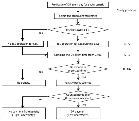
Figure 4.
DR participation process with ESS.
3. Indirect Energy Trading with the Non-Cooperative Game
3.1. Indirect Energy Trading with Incomplete Information
The results of the suggested strategies exhibit relatively high uncertainties, except for the condition with rare DR signals (Scenario 1), and this shows that, if a DR event happens more frequently than is typical, a rational participant would choose Strategy 1. Even though the results could encourage producers to participate in the DR program with their ESS, it would not be especially tempting to participants in light of the high uncertainty.
Kim et al. [23] suggested that prosumers could trade their electricity in a microgrid (MG) under peer-to-peer (P2P) conditions. However, in the case of IET as suggested in this work, surplus electricity is only shared through ESS systems. Moreover, IET does not affect the utility or retailer, but only the distribution system. Thus, if the prosumers make reasonable payments to the distributed system operator, such as those for connection charges, IET could feasibly be profitable.
The IET is based on the game that is conducted by considering the needs of each player who complies with the DR signal. Furthermore, the DR prediction for each player will be different, so some participants whose prediction are accurate will profit by complying with the DR signal, and others will fail to respond. The object of the game is derived from this mismatch. A failing actor might want to obtain some surplus electricity from other players in order to comply with the DR signal, even though the price is a little high. In this manner, participants who predict the DR signal successfully will sell their unused electricity during the DR event if they have any extra electricity after responding to the DR signal. Success and failure rates would be comparable for participants whose prediction ability is equal. Thus, each participant would choose to play the game if it could reduce uncertainty, since that would ensure that total benefits are increased.
From an economic perspective, each DR participant becomes a prosumer who could be both seller and buyer, meaning that, if they need more electricity for their DR signal response, they will function as a buyer. In contrast, they will become a seller if they have surplus electricity. Thus, if the indirect trading fee is slightly higher than the retail price, IET becomes feasible from an economic standpoint. For example, if the prosumer could lessen the uncertainty of DR participation by participating in IET, and the entire expected payoff after IET is increased, they would gladly buy the electricity despite the slightly higher price. Likewise, when they become a seller, they are willing to participate in energy trading, as the price is higher than the retail price. In short, a rational player will participate in the energy trading game if the condition in Equation (2) is satisfied:
where is the expected payoff with the game, is the expected payoff without the game, and is the additional cost from participating in the game.
To sum up, an IET occurs when a DR signal is dispatched, where some participants are unlikely to respond to the DR. Furthermore, since each participant’s DR prediction success rate is assumed to be the same, each participant becomes either a buyer or a seller every time a DR event occurs. The overall schematic of the IET is illustrated in Figure 5, and the DR event n is determined by the scenario. For example, n = 5 for scenario 1, n = 15 for scenario 2, and n = 25 for scenario 3.
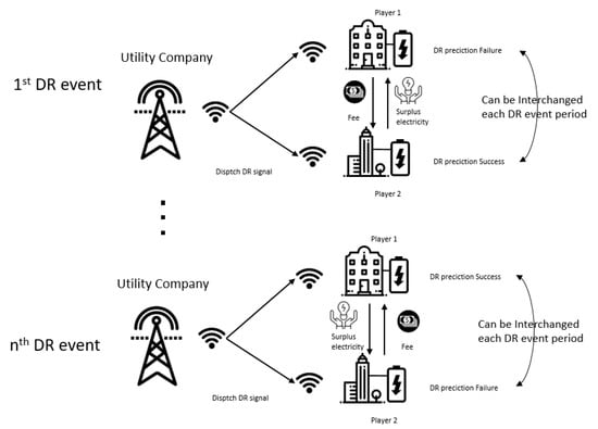
Figure 5.
Schematic of Indirect Energy Trading.
3.2. Non-Cooperative Game Framework
3.2.1. Components of the Non-Cooperative Game
In general, a game is made up of the set of players, the payoff, and the strategy. At first, DR participants will play this game to realize a better-than-expected payoff by decreasing the uncertainty of DR participation. Thus, the payoff for each player will be the incremental payoff for DR engagement. Finally, the strategy set is defined as which means that player will choose the strategy () and the strategy is related to the amount of the DR register capacity with the ESS.
3.2.2. Probability Distribution
For the game, we consider the scenario conditions for MC simulation noted as , and the probability of the scenario is:
As the game is incomplete, the player will choose a strategy without knowing the other players’ strategies and the strategic probability player and will choose each strategy and with scenario is defined as , and the probability set is:
In addition, we define the strategy profile in which player will choose strategy and player will choose strategy regardless of the scenarios, and , and are calculated as:
where
3.2.3. Expected Payoff
From the Probability Distribution, we can define the expected payoff function for each player when their strategy is or , and this payoff function will be used to find the N.E.:
where is the other player’s strategy (). The conditional probability is defined for a player using the strategy and player using the strategy :
The conditional payoff of a player is defined as
where is the additional expected payoff resulting from participating in the game, and is the transaction fee resulting when player buys from player . Similarly, is the transaction fee resulting when player sells to player . Those fees should satisfy these constraints:
As two players incur the transaction fees, the total transaction fee should be zero, as shown by (11). Next, the total transaction fee should be the sum of transaction fees for total time periods and DR event days (12). Finally, the transaction amount during a specific time slot should be determined by multiplying the amount of energy conveyed and the price at that time (13). signifies the amount of energy traded in time slot , and the price is slightly higher than is the retail price, , as mentioned in Section 3.1.
Likewise, we can find the expected payoff for player with strategy as:
where,
4. Case Study and Results
For the N.E. of the non-cooperative IET, consider that two players are under symmetric conditions for convenience. Furthermore, only three strategies are used (as described in Section 2.3), i.e., . The load data used are from buildings on the campus of Gwangju Institute of Science and Technology (GIST) in the Republic of Korea. The participation and settlement of the DR market are based on the electricity market rules of Korea [30].
Two players participate in the reliability DR program with 500 kWh ESS capabilities, and their uncertainty without the game is as shown in Table 3. Thus, the expected payoff without a non-cooperative game is calculated from the product of uncertainty and payments.
Table 3.
Uncertainty determined for strategies 1–3.
As Strategy 3 did not allow operation of the ESS for five days before the DR signal was dispatched, opportunity costs should be considered. This means that, if it did not participate in the DR with its ESS, the producer will receive the opportunity costs through arbitrage. Thus, their expected payoff is negative for frequent DR signals with Scenario 3 because they did not operate their ESS in preparation for 25 days of DR events.
4.1. Simulation Condition and Expected Payoff
The probability of each scenario is assumed based on the operational results (Table 1), and each probability is:
From Equations (4), (5), (8), (10), (14), and (16), each player has equal probability conditions due to the symmetry:
Furthermore, the results of the case study (Table 4) show that if almost any player will choose Strategy 3 and, if , almost any player will choose Strategy 1. However, the characteristics of the players also influence their strategy. For example, a conservative actor will prefer Strategy 1 and a progressive actor will prefer Strategy 3, regardless of the scenario. Thus, the strategy probability is assumed as:
Table 4.
Expected payoff for each strategy in the Korean Republic Won (KRW).
Therefore, from two probability conditions, we can express as:
The conditional payoff can be obtained through MCS based on the assumed parameters.
Finally, we can calculate the expected payoff for each player:
4.2. Results in Strategic Form for N.E.
As the game is symmetric for each player the results of each player is same, and the results of each scenario are showed in (28)–(30). Thus, we can generalize the results of each player’s expected payoff with a strategic game form.
Table 5 shows the expected payoffs for each strategy of player and player for scenario , and results also show that the Nash equilibrium (N.E.) strategy is Strategy 2, and Table 6 shows the results of participating in indirect energy trading (IET).
Table 5.
Results of the game with Scenario 1, Scenario 2, and Scenario 3.
Table 6.
Comparison of uncertainties.
Thus, we can derive the results of Table 6 and Table 7 through the process of MCS. As MCS is a very effective tool for dealing with the uncertainty problem, we can confirm the validity of results in Table 6 and Table 7 by reflecting the actual performance in Korea to the parameters assumed in MCS.
Table 7.
Comparison of expected payoff.
The results show that participants could improve their expected payoff by participating in IET, and the results show reliability in decreasing uncertainty. The uncertainty is decreased by 0.1316, 0.4751, and 0.2510, respectively, for Scenarios 1–3, and these reductions are related to the amounts of the expected payoffs. The payoff shows the most significant rise in Scenario 2, which models the average situation in Korea, and the payoff increase is about 4,032,879 Korean Republic Won (KRW). Furthermore, the total increment in expected payoff resulting from IET is 7,280,741 KRW.
Thus, the proposed DR participation using ESS and IET methods as a valuable complement would be economically feasible under the DR market conditions in Korea, and could consequently help stimulate the DR market.
5. Conclusions
We have implemented the MCS technique to handle the uncertainty from randomness of DR dispatch. At first, we generated a probabilistic model to predict DR event times, and strategies were suggested for participation in DR using ESS. Proposed strategies are related to the CBL and the discharging pattern occurring before a DR event, and they utilize operational results. However, these strategies, except for the first one, have relatively high uncertainties (Table 3) when DR events occur on more than 15 days during a year. A high level of uncertainty is inevitable because of the low DR prediction performance; owing to uncertainty, the potential DR participants are reluctant to participate in a DR program. Therefore, as an alternative to the relatively high uncertainty, the IET method is proposed to allow the sharing of the extra energy contained in ESS. IET was used with the partially symmetric non-cooperative game, meaning that each player is unaware of the other’s DR participation strategy or DR prediction success. Moreover, a case study based on the MCS was conducted with GIST building data and a set of reasonable starting assumptions. The results of the case study show that the uncertainty is effectively reduced by using the IET method, despite the poor DR prediction performance. Thus, prosumers can participate in the DR program with their ESS and via IET, even though they are unable to predict the occurrence of the DR event reliably. However, as IET is conducted under P2P conditions, further study on the operation of the P2P-based market in Korea should be undertaken.
Author Contributions
Conceptualization, J.R. and J.K.; Data analysis, simulation and methodology framework development, J.R. and J.K.; Writing, review, and editing, J.R. and J.K. Project management and supervision, J.K. All authors have read and agreed to the published version of the manuscript.
Funding
This work was supported by the Korea Institute of Energy Technology Evaluation and Planning (KETEP) and the Ministry of Trade, Industry & Energy (MOTIE) of the Republic of Korea (No. 20171210200810).
Conflicts of Interest
The authors have no conflicts of interest to declare.
References
- John, J.S. A How-to Guide for Transactive Energy; Greentech Media Inc.: Cambridge, MA, USA, 2013; Available online: http://www.greentechmedia.com/articles/read/a-how-to-guide-for-transactive-energy (accessed on 6 January 2020).
- GridWise Transactive Energy Framework Version 1.0; The GridWise Architecture Council, US Department of Energy: Washington, DC, USA, 2015; Available online: https://www.gridwiseac.org/pdfs/te_framework_report_pnnl-22946.pdf (accessed on 6 January 2020).
- International Renewable Energy Policy Change and Market Analysis, Report of Korea Energy Economics Institute. 2018. Available online: http://www.keei.re.kr/web_keei/d_results.nsf/0/66E351F39B9CC585492583CE00294E53/$file/%EA%B8%B0%EB%B3%B8%202018-27_%EA%B5%AD%EC%A0%9C%20%EC%8B%A0%EC%9E%AC%EC%83%9D%EC%97%90%EB%84%88%EC%A7%80%20%EC%A0%95%EC%B1%85%EB%B3%80%ED%99%94%20%EB%B0%8F%20%EC%8B%9C%EC%9E%A5%EB%B6%84%EC%84%9D.pdf (accessed on 30 January 2020).
- D’Hulst, R.; Labeeuw, W.; Beusen, B.; Claessens, S.; Deconinck, G.; Vanthournout, K. Demand response flexibility and flexibility potential of residential smart appliances: Experiences from large pilot test in Belgium. Appl. Energy 2015, 155, 79–90. [Google Scholar] [CrossRef]
- Benefits of Demand Response in Electricity Markets and Recommendations for Achieving Them. U.S. Department of Energy, 2016. Available online: https://www.smartgrid.gov/files/Benefits_Demand_Response_in_Electricity_Markets_Recommendati_200608.pdf (accessed on 6 January 2020).
- Demand Response Market Status and Operational Information. KPX, Korea. Available online: http://dr.kmos.kr/web/list.do?boardType=06 (accessed on 6 January 2020).
- Kang, J.; Lee, S. Data-driven prediction of load curtailment in incentive-based demand response system. Energies 2018, 11, 2905. [Google Scholar] [CrossRef]
- Lee, W.; Kang, B.O.; Jung, J. Development of the energy storage system scheduling algorithm for simultaneous self-consumption and demand response program participation in South Korea. Energy 2018, 161, 963–973. [Google Scholar] [CrossRef]
- Kang, B.O.; Hwang, B.G.; Kwon, K.; Jung, J.S. Operational strategy of energy storage system (ESS) to participate in demand response (DR) market for industrial customer. New. Renew. Energy 2017, 13, 4–12. [Google Scholar] [CrossRef]
- ISO. Guide to the Expression of Uncertainty in Measurement; Corrected and Reprinted in 1995; ISO: Geneva, Switzerland, 1993. [Google Scholar]
- Cox, M.; Harris, P. The Planned Supplemental Guide to the GUM: Numerical Methods for Propagating Distributions, National Physical Laboratory, UK, 2001. Available online: http://www.npl.co.uk/ssfm/index.html (accessed on 30 January 2020).
- Harrison, R.L. Introduction to Monte Carlo Simulation. AIP Conf. Proc. 2010, 1204, 17–21. [Google Scholar] [PubMed]
- Siebert, B.R.L. Monte-Carlo Methods: Scope and Limitations, Estimation of Measurement Uncertainty by Means of Monte-Carlo Integration; Physikalisch-Technische Bundesanstalt: Braunschweig, Germany, 2001. [Google Scholar]
- Dobney, A.; Klinkerberg, H.; Souren, F.; Van Borm, W. Uncertainty calculations for amount of chemical substance measurements performed by means of isotope dilution mass spectrometry as part of the PERM project. Anal. Chim. Acta 2000, 420, 89–94. [Google Scholar] [CrossRef]
- Hao, H. Modeling Dynamic Demand Response Using Monte Carlo Simulation and Interval Mathematics for Boundary Estimation. IEEE Trans. Smart Grid 2015, 6, 2704–2713. [Google Scholar] [CrossRef]
- Jonathan, A.S. Demand Response Contracts as Real Options: A Probabilistic Evaluation Framework Under Short-Term and Long-Term Uncertainties. IEEE Trans. Smart Grid 2016, 7, 868–878. [Google Scholar] [CrossRef]
- Heng, S. Data-Driven Uncertainty Quantification and Characterization for Household Energy Demand across Multiple Time-Scales. IEEE Trans. Smart Grid 2019, 10, 3092–3102. [Google Scholar] [CrossRef]
- Mohsenian-Rad, A.H.; Wong, V.W.S.; Jatskevich, J.; Schober, R.; Leon-Garcia, A. Autonomous demand side management based on game-theoretic energy consumption scheduling for the future smart grid. IEEE Trans. Smart Grid 2010, 1, 320–331. [Google Scholar] [CrossRef]
- Sheikhi, A.; Rayati, M.; Bahrami, S.; Ranjbar, A.M.; Sattari, S. A cloud computing framework on demand side management game in smart energy hubs. Electr. Power Energy Syst. 2015, 64, 1007–1016. [Google Scholar] [CrossRef]
- Serrano, R. Cooperative Games: Core and Shapley Value. In Encyclopedia of Complexity and Systems Science; Springer: Berlin, Germany, 2017; Available online: https://www.brown.edu/Departments/Economics/Faculty/serrano/pdfs/2008ECSS.pdf (accessed on 6 January 2020).
- Wang, H. Incentivizing energy trading for interconnected microgrids. IEEE Trans. Smart Grid 2018, 9, 2647–2657. [Google Scholar] [CrossRef]
- Li, J.; Wang, J.; Zhang, Y.J.A. Distributed transactive energy trading framework in distribution networks. IEEE Trans. Power Syst. 2018, 33, 7215–7227. [Google Scholar] [CrossRef]
- Kim, H.; Lee, J.; Bahrami, S.; Wong, V.W.S. Direct energy trading of microgrids in distribution energy market. IEEE Trans. Power Syst. 2020, 35, 639–651. [Google Scholar] [CrossRef]
- Adika, C.O.; Wang, L. Non-cooperative decentralized charging of homogeneous households’ batteries in a smart grid. IEEE Trans. Smart Grid 2014, 5, 1855–1863. Available online: https://arxiv.org/ftp/arxiv/papers/1911/1911.06500.pdf (accessed on 6 January 2020). [CrossRef]
- Wang, J.; Dou, X.; Guo, Y.; Shao, P.; Zhang, X. Purchase strategies for power retailers based on the non-cooperative game. Energy Procedia 2019, 158, 6652–6657. [Google Scholar] [CrossRef]
- Atzeni, I.; Ordonez, L.G.; Scutari, G.; Palomar, D.P.; Fonollosa, J.R. Noncooperative day-ahead bidding strategies for demand-side expected cost minimization with real-time adjustments: A GNEP approach. IEEE Trans. Sig. Process 2014, 62, 2397–2412. [Google Scholar] [CrossRef]
- Motalleb, M.; Ghorbani, R. Non-cooperative game-theoretic model of demand response aggregator competition for selling stored energy in storage devices. Appl. Energy 2017, 202, 581–596. [Google Scholar] [CrossRef]
- Wang, G.; Zhang, Q.; Li, H.; McLeellan, B.C.; Chen, S.; Li, Y.; Tian, Y. Study on the promotion impact of demand response on distributed PV penetration by using non-cooperative game theoretical analysis. Appl. Energy 2017, 185, 1869–1878. [Google Scholar] [CrossRef]
- Van de Schoot, R.; Broere, J.J.; Perryck, K.H.; Zondervan-Zwijnenburg, M.; van Loey, N.E. Analyzing small data sets using Bayesian estimation: The case of posttraumatic stress symptoms following mechanical ventilation in burn survivors. Eur. J. Psychotraumatol 2015, 6, 25216. [Google Scholar] [CrossRef] [PubMed]
- Electricity Market Rules, KPX. Available online: https://www.kpx.or.kr/eng/contents.do?key=299 (accessed on 6 January 2020).


© 2020 by the authors. Licensee MDPI, Basel, Switzerland. This article is an open access article distributed under the terms and conditions of the Creative Commons Attribution (CC BY) license (http://creativecommons.org/licenses/by/4.0/).