Abstract
An energy-management system requires accurate prediction of the electric load for optimal energy management. However, if the amount of electric load data is insufficient, it is challenging to perform an accurate prediction. To address this issue, we propose a novel electric load forecasting scheme using the electric load data of diverse buildings. We first divide the electric energy consumption data into training and test sets. Then, we construct multivariate random forest (MRF)-based forecasting models according to each building except the target building in the training set and a random forest (RF)-based forecasting model using the limited electric load data of the target building in the test set. In the test set, we compare the electric load of the target building with that of other buildings to select the MRF model that is the most similar to the target building. Then, we predict the electric load of the target building using its input variables via the selected MRF model. We combine the MRF and RF models by considering the different electric load patterns on weekdays and holidays. Experimental results demonstrate that combining the two models can achieve satisfactory prediction performance even if the electric data of only one day are available for the target building.
1. Introduction
The continuing environmental problems caused by the enormous amount of carbon dioxide produced by the burning of fossil fuels, such as coal and oil, for energy production has resulted in considerable focus on smart grid technologies owing to their effective use of energy [1,2]. A smart grid is an intelligent electric power grid that combines information and communication technology with the existing electric power grid [3]. The smart grid can optimize energy use by sharing electric energy production and consumption information with consumers and suppliers in both directions and in real time [4]. The most fundamental approach for sustainable development of smart grids is electric power generation using renewable energy sources, such as photovoltaic and wind energy [5,6]. Furthermore, an energy management system (EMS) in smart grids requires an optimization algorithm for the advanced operation of an energy storage system (ESS) [7]; it also has to plan various strategies by considering consumer-side decision making [8].
Artificial intelligence (AI) technology-based applications are a highly relevant area for smart grid control and management [6,7,8]. In particular, short-term load forecasting (STLF) is a core technology of the EMS [9]; moreover, accurate electric load forecasting is required for stable and efficient smart grid operations [10]. From the perspective of a supplier, it is challenging to provide optimal benefits in a cost-effective analysis while storing a large amount of electric energy in the ESS; however, the smart grid can plan effectively by predicting future electric energy consumption and receiving the required energy from internal and external energy sources [11]. It is also possible to optimize the renewable energy generation process [11,12]. From the perspective of a consumer, the EMS can quickly cope with situations such as blackouts and can help to save energy costs because it confirms the electric energy consumption and peak hours during the day [12].
Electric energy consumption patterns are complicated according to the types of buildings [13]; moreover, the electric energy consumption is frequently changed owing to uncertain external factors [14]. Therefore, it is challenging to predict the exact electric energy consumption in buildings [15]. Besides, when forecasting electric energy consumption, the complex correlations associated with an electric load between the current time and the previous time should be appropriately considered [7,11]. To adequately reflect previously uncertain external factors and electric energy consumption, AI techniques can be used to predict future building electric energy consumption based on diverse information, such as historical electric loads, locations, populations, weather factors, and events [16]. Moreover, the importance of multistep-ahead electric load forecasting has increased to quickly determine new uncertainties in power systems [17].
Most AI techniques use large amounts of data to construct STLF models. However, as sufficient electric load data of buildings connected to smart grids for a short time or new/renovated buildings are not collected, it is challenging to construct STLF models using these data sets. We defined this problem of lack of data as a cold-start problem. The cold-start problem [18] can occur in computer-based information systems that require automated data modeling. In particular, this problem involves the issue where the system cannot derive inferences from insufficient information regarding users or items. In future, because of the expansion of the smart grid market, it is expected that new data sets will be collected from newly constructed or renovated buildings. Hence, EMSs require a novel building electric energy consumption forecasting model that can be applied to these buildings.
In this paper, we propose a novel STLF model that combines random forest (RF) models while considering two cases (i.e., weekdays and holidays) to solve the cold-start problem. To achieve this, we first collected sufficient electric energy consumption data sets from 15 buildings. The collected data sets were divided into training and test sets; moreover, we developed a transfer learning-based STLF model based on multivariate random forests (MRF) in the training set. We also constructed a RF-based STLF model using the building electric energy consumption data of only 24 h and then combined the two models by considering the schedule. Consequently, we assumed the building electric energy consumption for only 24 h in the test set and performed multistep-ahead hourly electric load forecasting (24 points) of the target building to prepare for uncertainty.
The rest of this paper is organized as follows: in Section 2, we review several STLF models based on AI techniques using sufficient and insufficient data sets, respectively. In Section 3, we describe the input variable configuration for STLF models. In Section 4, we describe the RF-based STLF model construction in detail. Section 5 presents and discusses the experimental results to evaluate the prediction performance of the proposed model. In Section 6, we provide a conclusion and future research directions.
2. Related Works
In this section, we introduce the research on electric energy consumption forecasting for buildings with and without sufficient data sets. Table 1 summarizes the information about the selected papers, and these studies are described in detail subsequently.

Table 1.
Summary of several approaches for building electric energy consumption forecasting (MLR: multiple linear regression, SVR: support vector regression, GBM: gradient boosting machine, RF: random forest, SAE: stacked autoencoder, ELM: extreme learning machine, GA: genetic algorithm, LSTM: long short-term memory, PDRNN: pooling-based deep recurrent neural network, ANN: artificial neural network, CNN: convolutional neural network, GAN: generative adversarial network, BPNN: backward propagation neural network).
Several studies have predicted electric energy consumption for buildings with sufficient data sets based on traditional machine-learning and deep-learning (DL) methods. Candanedo et al. [19] proposed data-driven prediction models for a low-energy house using the data from home appliances, lighting, weather conditions, time factors, etc. They used multiple linear regression (MLR), support vector regression (SVR), RF, and gradient boosting machine (GBM) to construct 10 minute-interval electric energy consumption forecasting models. They confirmed that time factors were essential variables to build the prediction models; moreover, the GBM model exhibited better prediction performance than other models. Wang et al. [20] presented an hourly electric energy consumption forecasting model for two institutional buildings based on RF. They considered time factors, weather conditions, and the number of occupants as the input variables of the RF model. They compared the prediction performance of the RF model with that of the SVR model and confirmed that the RF model presented better prediction performance than the SVR model. Li et al. [21] proposed an extreme stacked autoencoder (SAE), which combined the SAE with an extreme learning machine (ELM) to improve the prediction results of building energy consumption. The electric energy consumption data were collected from one retail building in Fremont, CA. The authors predicted the building electric energy consumption at 30 min and 60 min intervals and compared the prediction performance of their proposed model with that of backward propagation neural network (BPNN), SVR, generalized radial basis function neural network, and MLR. Their proposed model demonstrated better prediction performance than other models. Almalaq et al. [22] presented a hybrid prediction model based on a genetic algorithm (GA) and long short-term memory (LSTM). GA was employed to optimize the window size and the number of hidden neurons for the LSTM model construction. Their proposed model predicted two public data sets of residential and commercial buildings and compared the prediction performance with autoregressive integrated moving average (ARIMA), decision tree (DT), k-nearest neighbor, artificial neural network (ANN), GA-ANN, and LSTM models. They confirmed that their proposed model exhibited better prediction performance than other models.
Several studies reported the construction of electric energy consumption forecasting models for buildings with insufficient data sets based on pooling, transfer learning, and data generation. Shi et al. [23] proposed a household electric load forecasting model using a pooling-based deep recurrent neural network (PDRNN). The pooling method was used to overcome the limitation of the complexity of household electric loads, such as volatility and uncertainty. Then, LSTM with five layers and 30 hidden units in each layer was employed to build an electric load-forecasting model using the pooling method. They compared the prediction performance of the PDRNN with that of ARIMA, SVR, recurrent neural network (RNN), etc. and confirmed that their proposed method outperformed ARIMA by 19.5%, SVR by 13.1%, and RNN by 6.5% in terms of the root mean square error. Ribeiro et al. [24] proposed a transfer-learning method, called Hephaestus, for cross-building electric energy consumption forecasting based on time-series multi-feature regression with seasonal and trend adjustments. Hephaestus was applied in the pre- and post-processing phases; then, standard machine learning algorithms such as ANN and SVR were used. This method adjusted the electric energy consumption data from various buildings by removing the effects of time through time-series adaptation. It also provided time-independent features through non-temporal domain adaptation. The authors confirmed that Hephaestus can improve electric energy consumption forecasting for a building by 11.2% by using additional electric energy consumption data from other buildings. Hooshmand and Sharma [25] constructed a transfer learning-based electric energy consumption forecasting model in small data set regimes. They collected publicly available electric energy consumption data and classified different types of customers. Then, normalization was utilized for training the trends and seasonality of time series efficiently. They built a convolutional neural network (CNN) architecture through the pre-training step that learns from a public data set with the same type of buildings as the target building. Subsequently, they retrained only the last fully connected layer using the data set of the target building to predict the energy consumption data of the target building. They demonstrated that their proposed model consistently demonstrated lower prediction performance error when compared to seasonal ARIMA, fresh CNN, and pre-trained CNN models. Tian et al. [26] proposed parallel building electric energy consumption forecasting models based on generative adversarial networks (GANs). They initially generated the parallel data through GAN by using a small number of the original data sets and then configured the mixed data set, which included the original data and the parallel data. Finally, they utilized the mixed data set to train several machine learning algorithms such as BPNN, ELM, and SVR. Experimental results exhibited that the parallel data consisted of similar distributions of the original data, and the prediction models trained by the mixed data set demonstrated better prediction performance than those trained using the original data, information diffusion technology, heuristic mega-trend-diffusion, and bootstrap methods.
The differences between the methods described above and our method are as follows:
The forecasting models in previous studies [19,20,21,22] presented excellent prediction performance using a sufficient data set of target buildings. However, our forecasting model can exhibit a satisfactory prediction performance even if the electric load data of the target building is insufficient.
The forecasting models in previous studies [19,20,21,22,23,24,26] could not predict the electric loads for various buildings. However, our forecasting model predicts the electric loads for 15 buildings; consequently, it can be considered as a generalized forecasting model.
The previous studies based on DL techniques [21,22,23,25,26] demonstrate a certain amount of computational cost to optimize the various hyperparameters of DL models for the target building. We use the RF with minimal tuning of hyperparameters to construct satisfactory forecasting models for several buildings.
The previous studies based on transfer learning [24,25] considered the types of the building to construct the forecasting models. However, we built a transfer learning-based forecasting model even without knowledge of the type of buildings. Besides, even if the electric load of only 24 h for the target building is known, our forecasting model can predict multistep electric load forecasting.
3. Input Variable Configuration
Our goal is to predict the electric energy consumption of buildings that were recently built. To address this issue, we constructed two STLF models, one using the sufficient electric load data of other buildings and the other using the limited electric load data of the target building. In this section, we describe the construction of input variables for practical model training. Section 3.1 describes the electric energy consumption data sets of the 15 buildings that we collected. Section 3.2 shows the input variable configuration for the RF-based forecasting model using the small data set of the target building. Section 3.3 exhibits the input variable configuration for the transfer learning-based forecasting models using the sufficient data sets from different buildings.
3.1. Data Sets of Electric Energy Consumption from Buildings
We randomly received the hourly electric energy consumption data collected from smart meters connected with 15 sites from the Korea Electric Power Corporation (KEPCO). One smart meter, which is installed per site, usually represents one building or a couple of connected buildings. In this paper, we defined a smart meter as a building. The period of data collection was from 1 January 2015 to 31 July 2018. As the collected building data were provided under anonymity and because of the de-identification owing to privacy, we could not determine the types, characteristics, and locations of the buildings. The collected smart meter data had an average missing value rate of 0.6%; we imputed these missing values using linear interpolation. The statistical analysis of the collected smart meter data for each building is listed in Table 2.
Table 2.
Statistics of electric energy consumption data from each building (Unit: kWh).
Herein, we made one assumption. Even though we have sufficient electric energy consumption data sets for other buildings, we have the electric energy consumption data set of only 24 h for the target building. Thus, as we know the electric load of the target building for only 24 h (24 points), we predicted the electric energy consumption for the subsequent 24 h.
3.2. Case 1: Time Factor-Based Forecasting Modeling
As mentioned above, we assumed that the electric energy consumption data of only 24 h for the target building was known. Hence, we explain the input variable configuration for the prediction model utilizing the electric energy consumption data of only 24 h. Generally, while constructing a STLF model, various factors, such as time factors, weather information, and historical electric loads, are reflected as input variables [27,28]. However, we cannot utilize weather information as an input variable because we do not know the location of the buildings. The historical electric load is used to reflect recent trends and patterns [28,29]; moreover, it can be applied when it is composed of sufficient data sets. However, as we assumed that the historical electric load is composed of data of only 24 h, reflecting on the historical electric load is inappropriate. This implies that we do not know any recent trends or patterns. In the case of time factors, there are various factors, namely month, day, hour, day of the week, and holiday. However, the data set was too small to effectively reflect the characteristics of months, days, days of the week, and holidays. Therefore, we considered only “hour” as an input variable to construct the STLF model.
However, in the case where 11 pm and 12 am of the subsequent day are adjacent, but the difference is 23, it is challenging to train the input variable of the STLF model effectively. Thus, we use Equations (1) and (2) to enhance the sequence data in the one-dimensional space to the continuous data in the two-dimensional space [11,30]. These variables can more adequately reflect the continuous characteristic, similar to the shape of the clock, as shown in Figure 1.
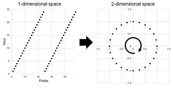
Figure 1.
Example of the enhancement of one-dimensional space to two-dimensional space.
Table 3 and Table 4 lists the results of the statistical analysis of the building electric energy consumption for one-dimensional and two-dimensional spaces. In Table 3, we can observe that the two-dimensional space reflects the building electric energy consumption more effectively than the one-dimensional space. In Table 4, we can see that almost of p-values of the F-statistic are , which are highly significant. This means that at least, one of the predictor variables is significantly related to the outcome variable. We used 24-hour information to construct the STLF model and then applied the same time information to predict the building electric energy consumption over the next 24 h.
Table 3.
R-squared statistics and standard error for each building.
Table 4.
F-statistics and p-value for each building.
3.3. Case 2: Transfer Learning-Based Forecasting Modeling
In addition to the electric energy consumption data set of the target building for only 24 h, we also have sufficient electric energy consumption data sets of other buildings. Hence, we can reflect on various characteristics to use as input variables for a transfer learning-based model construction. Consequently, we used a time factor and historical electric load as input variables. We first divided the electric energy consumption data of all buildings into training and test sets. In the training set, we used the electric energy consumption data of different buildings to train the transfer learning-based STLF models and these models were applied to the electric energy consumption data of the target building when it was used in the test set. For time factors, we used the month, week, day, hour, day of the week, and holiday information. In the case of months, weeks, days, and days of the week, we enhanced the time factors from the one-dimensional space to two-dimensional space, as shown in Equations (3) to (10) [30,31]. Here WN is the week number based on the ISO 8601 standard [32], and LDM represents the last day of the month.
The holidays included Saturdays, Sundays, and national holidays and exhibited predominantly low electric energy consumption during working hours, unlike working days [33]. In the case of holidays, we used one-hot encoding to reflect the property as “1” on the holiday and “0” otherwise. Hence, we applied nine time factors as input variables at the prediction time point.
In addition, we applied not only the historical electric load data but also the day of the week and holiday, which are a part of the data, to reflect both the historical electric load of the building and its characteristics. Consequently, we configured 15 input variables at the prediction point time. Table 5 lists the information on these variables; where D represents the day.
Table 5.
List of input variables for the transfer learning-based forecasting model.
As our goal is to predict all-time points 24 h later, we constructed all the input variables by utilizing each input variable for the prediction time point. Thus, we used a total of 360 input variables, i.e., (15 (number of input variables) 24 (prediction time points)) for the STLF model construction, as shown in Figure 2.
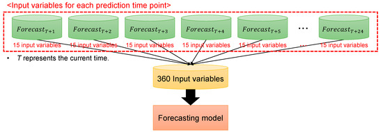
Figure 2.
Input variable configuration for the transfer learning-based forecasting model.
4. Forecasting Model Construction
In this section, we describe the STLF model construction using the limited data set of the target building and the data sets of other buildings; moreover, we also present the method to select the prediction value derived from the transfer learning-based model. In addition, we combined the two STLF models and thus present a total of 15 STLF models. Figure 3 illustrates a brief system architecture of our proposed model.
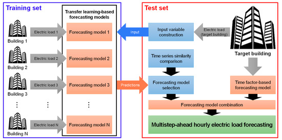
Figure 3.
Overall system architecture.
4.1. Case 1: Time Factor-Based Forecasting Model
To construct an STLF model using only “hour” as an input (independent) variable, we used one statistical technique and two machine learning algorithms. Even though SVM, DL, and boosting methods exhibit excellent prediction performance in STLF [7,8,9,34,35,36,37], they require a significant amount of time to optimize the various hyperparameters and also require sufficient data sets. We did not consider these methods because we constructed an STLF model using a data set from the building electric energy consumption data of only 24 h. Thus, we considered MLR, DT, and RF, which allow simple model construction and exhibit satisfactory prediction performance [38,39]. We used two-time factors, namely, and as independent variables and the electric energy consumption for the target building as the dependent (output) variable. Therefore, we predicted multistep-ahead hourly electric loads using the time factor-based forecasting model via a sliding window time series analysis, as shown in Figure 4.
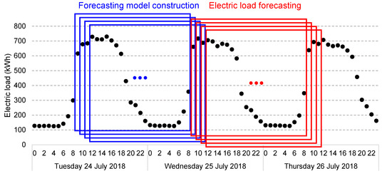
Figure 4.
Example of multistep-ahead electric load forecasting via a sliding window method.
4.1.1. Multiple Linear Regression (MLR)
MLR is a common statistical technique that is widely used in many STLF models [39]. MLR [39] analyzes the relationship between a continuous dependent variable and one or more independent variables. The value of the dependent variable can be predicted using a range of values of the independent variables based on an identity function that describes, as closely as possible, the relationship between these variables. In addition, MLR determines the overall fit of the prediction model and the relative contribution of each independent variable to the total variance. Equation (11) represents the method to construct the MLR-based STLF model. is the forecast energy consumption at time and is the intercept of population . and are population slope coefficients. By defining the weights of the MLR model based on and at the prediction time, we can construct a more sophisticated STLF model. Herein, , , and are calculated when the prediction model is built by using the electric loads at the previous one day from the prediction points. Because our model focuses on the prediction of multistep electric loads using a sliding window method, the weights of , , and are adjusted every hour.
4.1.2. Decision Tree (DT)
A DT [40] is used to construct classification or regression models in the form of a tree structure. It separates a data set into smaller subsets while an associated DT is being incrementally extended. The final result is a tree with a decision node that has two or more branches and a leaf node that denotes a classification or decision. The topmost decision node in a tree corresponds to the best predictor, called root node. DTs can present a higher explanatory power because they determine the independent variables that have a more powerful impact when predicting the values of the target variable [41]. However, continuous variables (i.e., building electric energy consumption) used in the prediction of the time series are considered as discontinuous values. Hence, prediction errors are likely to occur near the boundary of separation.
4.1.3. Random Forest (RF)
RF [41] is an ensemble learning method that combines different DTs that classify a new instance by the majority vote. Each DT node utilizes a subset of attributes randomly selected from the original set of characteristics. As RF can handle large amounts of data effectively, it exhibits a high prediction performance in the field of STLF [14]. Besides, when compared to other AI techniques, such as DL and gradient-boosting algorithms, RF requires less fine tuning of its hyperparameters [42]. The basic hyperparameters of RF include the number of trees to grow (nTree) and the number of variables randomly sampled as candidates at each split (mTry). The correct value for nTree is usually not of much concern because increasing the number of trees in the RF raises the computational cost and does not contribute significantly to prediction performance improvement [14,41]. However, it is interesting to note that picking too small a value of mTry can lead to overfitting. We consider only two input variables, mTry and nTree, which are set to 2 and 128 [43], respectively.
4.2. Case 2: Transfer Learning-Based Forecasting Model
Transfer learning [44] is a process that utilizes the knowledge gained while solving one issue to a different but related issue. To achieve this, a base machine-learning method is first trained on a base data set or task. Then, the method repurposes or transfers the learned features to the second target data set or task. This process can operate if the features are general and the intentions are suitable for both base and target tasks rather than being specific to the base task. We previously configured the input variable for transfer learning-based STLF model construction. We first divided the training and test sets. In the training set, we used electric energy consumption data of other buildings to train the transfer learning-based forecasting model. Then, the model predicted the multistep electric load for the target building using its input variables in the test set. Finally, we selected appropriate prediction results for the target building from the other 14 forecasting models. We describe the details in the subsections below.
4.2.1. Multivariate Random Forests (MRF)
Neural network techniques have been used to predict multistep electric loads [45,46,47]. However, they require scaling (e.g., robust normalization, standardization, and min-max normalization) before building a prediction model [11]. Thus, when the transfer learning-based STLF model is applied to the target building, the electric load of the target building can exhibit a different range than the electric load of other buildings. Consequently, if STLF models that are trained by scaling are used to predict future electric load for the target building, it is challenging to accurately apply them into the electric load range of the target building.
Consequently, we used MRF (when the number of output features > one) for transfer learning-based STLF model construction. MRF [48] can provide multivariate outcomes and can generate an ensemble of multivariate regression trees through bootstrap resampling and predictors subsampling for univariate RF. In MRF, node cost is measured as the sum of squares of the Mahalanobis distance, whereas in univariate trees (i.e., RF), the node cost is measured as the Euclidean distance (ED) [49]. MRF can provide excellent prediction performance without scaling for multiple output predictions [50,51]. Therefore, we used the input variables without scaling to train the MRF models and predicted the electric load of the target building using the input variable of the target building without scaling. To construct the MRF models, we set mTry and nTree as 120 (number of input variables/3) and 128, respectively [14]. Thus, when a total of 14 prediction results are derived from each MRF model, we did not use all of them and instead selected only one prediction result that exhibits the most similar time series through the similarity analysis between the target building and the other buildings. Then, we used the prediction result as the model that demonstrates the most similar time series to predict the electric load of the target building. Here, we consider a total of three techniques and describe the details in the subsections below.
4.2.2. Similarity Measures
We used three similarity measures, i.e., Pearson correlation coefficient (PCC), cosine similarity (CS), and ED, to analyze the similarity of the time series between the target building and other buildings. These methods are commonly used for similarity analysis [13].
PCC [52], which is a measure of the linear correlation between two variables, and , is the covariance of these variables divided by the product of the standard deviations in the data of equal or proportional scales. It has a value between +1 and −1, according to the Cauchy–Schwarz inequality, where +1 is a perfect positive linear correlation, 0 indicates no linear correlation, and −1 is a perfect negative linear correlation. For the paired data consisting of pairs, , which is a substituting estimation of the covariances and variances based on a sample, is defined according to Equation (12). Here, is the sample size, and are the individual sample points indexed with time . and are the sample means of and , respectively. For our experiments, because we considered hourly electric load for only 24 h, is 24. and are the hourly electric loads indexed with of the target and different buildings, respectively. Herein, we apply the prediction model of the building whose PCC is closest to one by comparing the target building with other buildings.
CS [53] indicates the similarity between vectors measured using the cosine of the angle between two vectors in the inner space. The cosine when the angle is is one, and the cosine of all other angles is smaller than one. Therefore, this value is used to determine the similarity of the direction, not the magnitude of the vector. The value is +1 when the two vectors are in exactly the same direction. The value is 0 when the angle is , and the value is −1 when the vectors are in completely opposite directions, i.e., an angle of . At this time, the size of the vector does not affect the value. The CS can be applied to any number of dimensions and is often used to measure similarity in a multidimensional amniotic space. Given the vector values of the attributes and , CS () can be expressed by the scalar product and magnitude of the vector, as shown in Equation (13). For our experiments, as mentioned earlier, is 24. and are the hourly electric loads indexed with of the target and different buildings, respectively. Herein, we apply the prediction model of the building whose CS is closest to one by comparing the target building with other buildings.
ED [54,55] is a common method for calculating the distance between two points. This distance can be used to define the Euclidean space, and the corresponding norm is called the Euclidean norm. A generalized term for the Euclidean norm is the norm or distance [55]. In a Cartesian coordinate system, where there are points and in Euclidean space, the distance between two points and is calculated using two Euclidean norms, which is defined according to Equation (14). The distance between any two points on the real line is the absolute value of the numerical difference of their coordinates. It is common to identify the name of a point with its Cartesian coordinate. When the two points and are the same, the distance value is zero. For our experiments, as mentioned earlier, is 24. and are the hourly electric loads indexed with of the target and different buildings, respectively. Herein, we apply the prediction model of the building whose ED is closest to zero by comparing the target building with other buildings.
4.3. Case 3: Combining Short-Term Load-Forecasting Models
We considered the following situations to apply more suitable forecasting models for each case. As mentioned above, the electric load patterns vary significantly depending on the days of the week and holidays [32]. For instance, in chronological sequence, the difference in electric loads between Friday and Saturday is large. The difference in electric loads between Sunday and Monday is also large. Therefore, if the time factor-based forecasting model predicts the electric load on the weekend by using the electric load on a weekday, the forecast value presents multiple error rates because it exhibits the weekday pattern. In addition, when constructing a time factor-based forecasting model by using only a low electric load, such as that on Sunday or a national holiday, it can cause high error rates because of a high electric load on Monday. To address these issues, we combined the time factor- and transfer-learning-based forecasting models. We applied the prediction models by considering two cases at the 24 prediction points and illustrated examples of the electric load forecasting using the combined STLF model in Figure 5 and hence we constructed a total of 15 STLF models, as shown in Table 6.
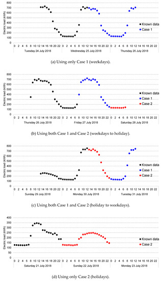
Figure 5.
Examples of multistep-ahead electric load forecasting using the combined short-term load forecasting (STLF) model by considering two cases.
Table 6.
Construction of various forecasting models (MLR: multiple linear regression, DT: decision tree, RF: random forest, MRF: multivariate random forests, PCC: Pearson correlation coefficient, CS: cosine similarity, ED: Euclidean distance).
- Case 1: For each prediction point, we applied the time vector-based forecasting model when both the prediction point and the day before the prediction point are weekdays.
- Case 2: For each prediction point, we applied the transfer learning-based forecasting model when the prediction point and/or the day before the prediction point are holidays.
5. Experimental Results
5.1. Performance Evaluation Metric
To evaluate the prediction performance of the proposed model, we used the mean absolute percentage error (MAPE), root mean square error (RMSE), and mean absolute error (MAE). The MAPE value usually presents accuracy as a percentage of the error and can be easier to comprehend than the other statistics because this number is a percentage [11,40]. The MAPE can be defined according to Equation (15). The RMSE is used to aggregate the residuals into a single measure of predictive ability, as shown in Equation (16). The RMSE is the square root of the variance, which denotes the standard error. The MAE is used to evaluate how close forecast or prediction values are to the actual observed values, as shown in Equation (17). The MAE is calculated by averaging the absolute differences between the prediction values and the actual observed values. The MAE gives the average magnitude of forecast error, while the RMSE gives more weight to the most significant errors. Lower values of MAPE, RMSE, and MAE indicate better prediction performance of the forecasting model. Here, is the number of observations and and are the actual and forecast values, respectively.
5.2. Prediction Performance Evaluation
To evaluate the performance of the forecasting models, we conducted the experiments with an Intel ® Core™ i7-8700k CPU with 32GB DDR4 RAM and preprocessed the datasets in RStudio version 1.1.453 with R version 3.5.1. We also carried out the construction of the forecasting models using ‘tree’ (DT), ‘randomForest’ (RF), and ‘MultivariateRandomForest’ (MRF) packages [49,56,57].
As we collected the electric energy consumption data from a total of 15 buildings, we used 15-fold cross-validations to evaluate the prediction performance. In the collected data, the periods of the training and test sets are from 1 January 2015 to 31 July 2017 and from 1 August 2017 to 31 July, 2018, respectively.
We reported training and testing times of the MRF models for each building in Table 7. The training time represents the time to train the MRF model in each building, and the testing time indicates the time for performing all predictions from the three transfer learning-based forecasting models (i.e., M04, M05, and M06).
Table 7.
Running times of the multivariate random forest (MRF) model in each building (Unit: second).
Because MAPE is a widely used error measurement metric in the electric load-forecasting literature, we presented all the results of multistep-ahead hourly electric load forecasting accuracy using the MAPE in Table 8, Table 9, Table 10, Table 11, Table 12, Table 13, Table 14, Table 15, Table 16, Table 17, Table 18, Table 19, Table 20, Table 21, Table 22 and Table 23. We also exhibited the average forecasting accuracy of multistep electric loads using RMSE and MAE results in Table 24 and Table 25, respectively.
Table 8.
Mean absolute percentage error (MAPE) comparison of forecasting models for Building 1 (a cooler color indicates a lower MAPE value, while a warmer color indicates a higher MAPE value).
Table 9.
MAPE comparison of forecasting models for Building 2 (a cooler color indicates a lower MAPE value, while a warmer color indicates a higher MAPE value).
Table 10.
MAPE comparison of forecasting models for Building 3 (a cooler color indicates a lower MAPE value, while a warmer color indicates a higher MAPE value).
Table 11.
MAPE comparison of forecasting models for Building 4 (a cooler color indicates a lower MAPE value, while a warmer color indicates a higher MAPE value).
Table 12.
MAPE comparison of forecasting models for Building 5 (a cooler color indicates a lower MAPE value, while a warmer color indicates a higher MAPE value).
Table 13.
MAPE comparison of forecasting models for Building 6 (a cooler color indicates a lower MAPE value, while a warmer color indicates a higher MAPE value).
Table 14.
MAPE comparison of forecasting models for Building 7 (a cooler color indicates a lower MAPE value, while a warmer color indicates a higher MAPE value).
Table 15.
MAPE comparison of forecasting models for Building 8 (a cooler color indicates a lower MAPE value, while a warmer color indicates a higher MAPE value).
Table 16.
MAPE comparison of forecasting models for Building 9 (a cooler color indicates a lower MAPE value, while a warmer color indicates a higher MAPE value).
Table 17.
MAPE comparison of forecasting models for Building 10 (a cooler color indicates a lower MAPE value, while a warmer color indicates a higher MAPE value).
Table 18.
MAPE comparison of forecasting models for Building 11 (a cooler color indicates a lower MAPE value, while a warmer color indicates a higher MAPE value).
Table 19.
MAPE comparison of forecasting models for Building 12 (a cooler color indicates a lower MAPE value, while a warmer color indicates a higher MAPE value).
Table 20.
MAPE comparison of forecasting models for Building 13 (a cooler color indicates a lower MAPE value, while a warmer color indicates a higher MAPE value).
Table 21.
MAPE comparison of forecasting models for Building 14 (a cooler color indicates a lower MAPE value, while a warmer color indicates a higher MAPE value).
Table 22.
MAPE comparison of forecasting models for Building 15 (a cooler color indicates a lower MAPE value, while a warmer color indicates a higher MAPE value).
Table 23.
Average MAPE comparison of forecasting models (a cooler color indicates a lower MAPE value, while a warmer color indicates a higher MAPE value).
Table 24.
Average root mean square error (RMSE) results of 15 forecasting models for each building (a cooler color indicates a lower RMSE value, while a warmer color indicates a higher RMSE value).
Table 25.
Average mean absolute error (MAE) results of 15 forecasting models for each building (a cooler color indicates a lower MAE value, while a warmer color indicates a higher MAE value).
In Table 8, Table 9, Table 10, Table 11, Table 12, Table 13, Table 14, Table 15, Table 16, Table 17, Table 18, Table 19, Table 20, Table 21, Table 22, Table 23, Table 24 and Table 25, a cooler color (blue) indicates lower MAPE, RMSE, and MAE values, while a warmer color (red) indicates higher MAPE, RMSE, and MAE values. To confirm the overall prediction performance of the forecasting models, we presented the average MAPE of different forecasting models and indicated the best accuracy in bold. In addition, a box plot for each forecasting model is shown in Figure 6, Figure 7, Figure 8, Figure 9, Figure 10, Figure 11, Figure 12, Figure 13, Figure 14, Figure 15, Figure 16, Figure 17, Figure 18, Figure 19 and Figure 20 using MAPE values for each prediction point. This means that the box, which is located below and exhibits the smaller range, is a more stable forecasting model.
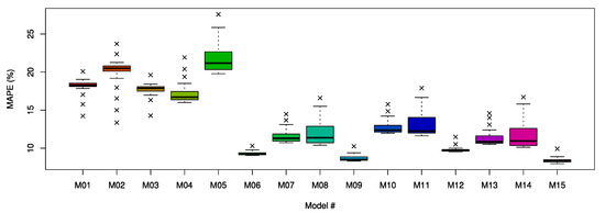
Figure 6.
Box plot of the mean absolute percentage error (MAPE) of forecasting models for Building 1.
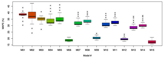
Figure 7.
Box plot of the MAPE of forecasting models for Building 2.
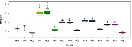
Figure 8.
Box plot of the MAPE of forecasting models for Building 3.
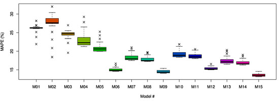
Figure 9.
Box plot of the MAPE of forecasting models for Building 4.
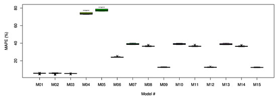
Figure 10.
Box plot of the MAPE of forecasting models for Building 5.
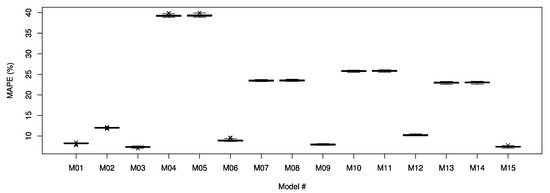
Figure 11.
Box plot of the MAPE of forecasting models for Building 6.
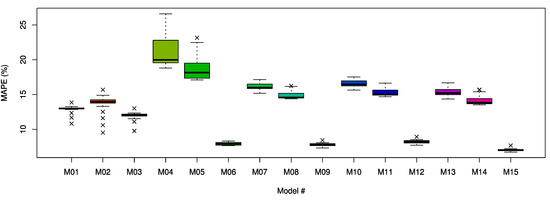
Figure 12.
Box plot of the MAPE of forecasting models for Building 7.
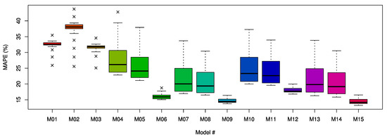
Figure 13.
Box plot of the MAPE of forecasting models for Building 8.
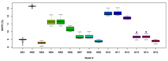
Figure 14.
Box plot of the MAPE of forecasting models for Building 9.
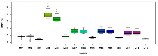
Figure 15.
Box plot of the MAPE of forecasting models for Building 10.
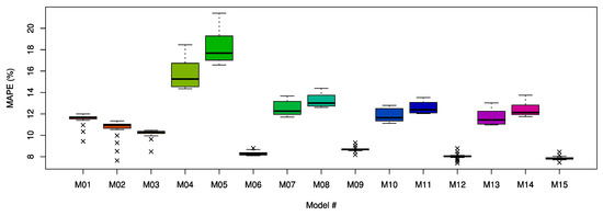
Figure 16.
Box plot of the MAPE of forecasting models for Building 11.
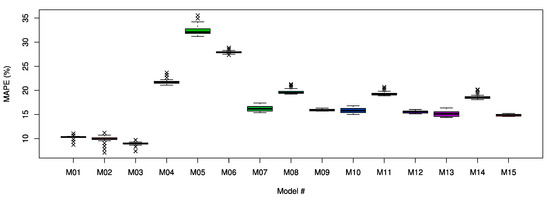
Figure 17.
Box plot of the MAPE of forecasting models for Building 12.
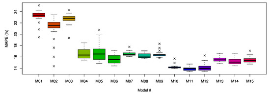
Figure 18.
Box plot of the MAPE of forecasting models for Building 13.
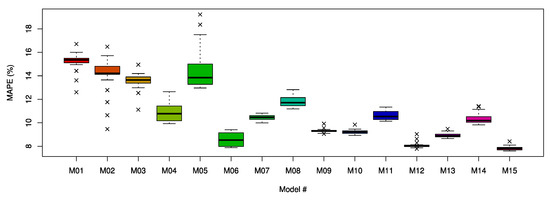
Figure 19.
Box plot of the MAPE of forecasting models for Building 14.
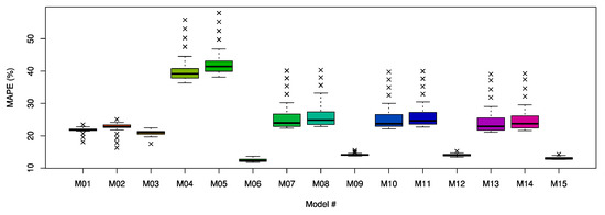
Figure 20.
Box plot of the MAPE of forecasting models for Building 15.
As shown in Table 8, Table 9, Table 10, Table 11, Table 12, Table 13, Table 14, Table 15, Table 16, Table 17, Table 18, Table 19, Table 20, Table 21, Table 22, Table 23, Table 24 and Table 25 and Figure 6, Figure 7, Figure 8, Figure 9, Figure 10, Figure 11, Figure 12, Figure 13, Figure 14, Figure 15, Figure 16, Figure 17, Figure 18, Figure 19 and Figure 20, the RF demonstrated the best prediction performance in the time factor-based forecasting models, and MRF_ED showed the best prediction performance in the transfer learning-based forecasting models. The reason why ED demonstrated the best performance is only because the distance of electric energy consumption between buildings was considered, unlike the PCC or CS; thus, it can reflect a similar range of electric energy consumption adequately when training the transfer learning-based forecasting model. Consequently, we can observe that M15 demonstrated better prediction performances than other forecasting models in most experiments. M15 is appropriate for solving the cold-start problem in STLF and used two tree-based methods; we called this model as SPROUT (solving cold start problem in short-term load forecasting using tree-based methods).
To demonstrate the superiority of the SPROUT model, we performed several statistical tests, such as Wilcoxon signed-rank and Friedman tests [58,59]. The Wilcoxon signed-rank test [58] is used to confirm the null hypothesis to determine whether there is a significant difference between two models. If the p-value is less than the significance level, the null hypothesis is rejected, and the two models are judged to have significant differences. The Friedman test [59] is a multiple comparison test that aims to identify significant differences between the results of two or more forecasting models. To verify the results of the two tests, we used all the MAPE values (15 (number of the buildings) 24 (prediction time points)) for each forecasting model. The results of the Wilcoxon test with the significance level set to 0.05 and the Friedman test are listed in Table 26. We can observe that the proposed SPROUT model significantly outperforms the other models because the p-value in all cases is below the significance level.
Table 26.
Results of the Wilcoxon and Friedman tests with SPROUT (solving cold start problem in short-term load forecasting using tree-based methods).
5.3. Discussion
The SPROUT model demonstrated the best performance in the majority of experiments, excluding certain buildings. Thus, we analyzed these cases in detail. In Figure 21, we can observe that Buildings 3, 5, 6, 9, and 10 illustrated no significant difference in weekday and weekend electric loads. As shown in Table 2 and Figure 21f, Building 12 was unable to reflect similar electric load patterns owing to the wide range of electric energy consumption data. Hence, the transfer learning-based forecasting models demonstrated unsatisfactory prediction performance. Therefore, despite the differences in weekday and weekend patterns, the time factor-based forecasting models showed better prediction performance.
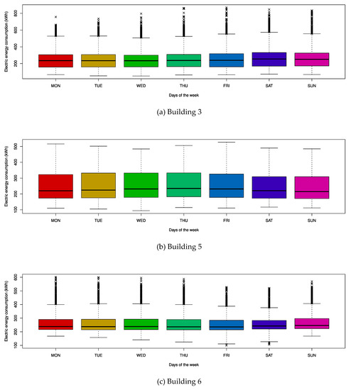
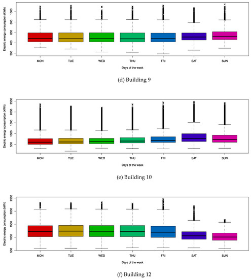
Figure 21.
Box plot of electric loads according to each day of the week.
Building 13 showed that M10 to M12 presented better prediction performance than other models because MLR could predict the building electric energy consumptions better than DT and RF. In addition, as listed in Table 20, Building 13 demonstrated a wide range of electric energy consumption data and also showed the highest electric energy consumption. Therefore, even when the ED was close, it was challenging to accurately derive the results of the transfer learning-based forecasting model. The electric load patterns of Building 15 were considerably similar to those of Building 8, as shown in the F test in Table 27. Therefore, as M06 demonstrated accurate predictions on both weekdays and weekends, it exhibited the lowest prediction error rate.
Table 27.
F test between Building 8 and Building 15.
6. Conclusions
When sufficient building electric energy consumption data are not available as in newly constructed or renovated buildings, it is difficult to train and construct superior STLF models. Nevertheless, electric load-forecasting models are required for efficient power management, even by considering such limited data sets. In this paper, we proposed a novel STLF model, called SPROUT, to predict electric energy consumption for buildings with limited data sets by combining time factor- and transfer learning-based forecasting models. We used MRF to construct transfer learning-based STLF models for each building by using sufficient building electric energy data and selected the model, which exhibited the most similar time-series pattern to predict the electric load of the target building. We also constructed STLF models based on RF by using the building electric energy consumption data of only 24 h and then used the two models depending on weekdays and holidays. To verify the validity and applicability of our model, we used MLR and DT to construct time factor-based forecasting models and compared their prediction performance. The experimental results showed that the RF-based STLF model presented a better prediction performance in the time factor-based forecasting model, and the MRF-based STLF model, by applying ED, exhibited a better prediction performance in the transfer learning-based forecasting model. By combining these models, our model (SPROUT) presented excellent prediction performances in MAPE, RMSE, and MAE results. The SPROUT showed an average MAPE value of 11.2 in the experiments and exhibited more accurate prediction performances of 5.9%p (MLR), 6.7%p (DT), and 4.6%p (RF) than time factor-based STLF models. It also showed more accurate prediction performances of 15.6%p (MRF_PCC), 16.9%p (MRF_CS), and 2.6%p (MRF_ED) than transfer learning-based STLF models. We demonstrated that the SPROUT can achieve better prediction performance than other forecasting models.
However, when electric load exhibited no significant difference in weekday and weekend electric loads in the building, the time factor-based STLF models outperformed our model. In addition, the transfer learning-based STLF models presented unsatisfactory prediction performance in the building with the highest electric energy consumption and hence our model cannot perform accurate electric load forecasting. To address these issues, we plan to consider additional electric load data over a period of time for performing weekly electric load pattern analysis and data normalization.
Author Contributions
All authors have read and agree to the published version of the manuscript. Conceptualization, J.M.; methodology, J.M. and J.K.; software, J.M.; validation, J.M., J.K., and P.K.; formal analysis, P.K. and E.H.; data curation, J.M. and J.K.; writing—original draft preparation, J.M.; writing—review and editing, E.H.; visualization, J.K.; supervision, E.H.; project administration, P.K. and E.H.; funding acquisition, P.K. and E.H.
Funding
This research was supported in part by the Korea Electric Power Corporation (grant number: R18XA05) and in part by Energy Cloud R&D Program (grant number: 2019M3F2A1073179) through the National Research Foundation of Korea (NRF) funded by the Ministry of Science and ICT.
Acknowledgments
We greatly appreciate the anonymous reviewers for their comments and suggestions.
Conflicts of Interest
The authors declare no conflict of interest.
References
- Cao, X.; Dai, X.; Liu, J. Building energy-consumption status worldwide and the state-of-the-art technologies for zero-energy buildings during the past decade. Energy Build. 2016, 128, 198–213. [Google Scholar] [CrossRef]
- Alani, A.Y.; Osunmakinde, I.O. Short-Term Multiple Forecasting of Electric Energy Loads for Sustainable Demand Planning in Smart Grids for Smart Homes. Sustainability 2017, 9. [Google Scholar] [CrossRef]
- Abbasi, R.A.; Javaid, N.; Khan, S.; ur Rehman, S.; Amanullah; Asif, R.M.; Ahmad, W. Minimizing Daily Cost and Maximizing User Comfort Using a New Metaheuristic Technique. In Workshops of the International Conference on Advanced Information Networking and Applications; Springer: Cham, Switzerland, 2019; pp. 80–92. [Google Scholar] [CrossRef]
- Nawaz, M.; Javaid, N.; Mangla, F.U.; Munir, M.; Ihsan, F.; Javaid, A.; Asif, M. An Approximate Forecasting of Electricity Load and Price of a Smart Home Using Nearest Neighbor. In Conference on Complex, Intelligent, and Software Intensive Systems; Springer: Cham, Switzerland, 2019; pp. 521–533. [Google Scholar] [CrossRef]
- Zhou, K.; Fu, C.; Yang, S. Big data driven smart energy management: From big data to big insights. Renew. Sustain. Energy Rev. 2016, 56, 215–225. [Google Scholar] [CrossRef]
- Bose, B.K. Artificial Intelligence Techniques in Smart Grid and Renewable Energy Systems—Some Example Applications. Proc. IEEE 2017, 105, 2262–2273. [Google Scholar] [CrossRef]
- Kim, J.; Moon, J.; Hwang, E.; Kang, P. Recurrent inception convolution neural network for multi short-term load forecasting. Energy Build. 2019, 194, 328–341. [Google Scholar] [CrossRef]
- Ahmad, A.S.; Hassan, M.Y.; Abdullah, M.P.; Rahman, H.A.; Hussin, F.; Abdullah, H.; Saidur, R. A review on applications of ANN and SVM for building electrical energy consumption forecasting. Renew. Sustain. Energy Rev. 2014, 33, 102–109. [Google Scholar] [CrossRef]
- Monfet, D.; Corsi, M.; Choinière, D.; Arkhipova, E. Development of an energy prediction tool for commercial buildings using case-based reasoning. Energy Build. 2014, 81, 152–160. [Google Scholar] [CrossRef]
- Parhizi, S.; Khodaei, A.; Shahidehpour, M. Market-Based Versus Price-Based Microgrid Optimal Scheduling. IEEE Trans. Smart Grid 2018, 9, 615–623. [Google Scholar] [CrossRef]
- Moon, J.; Park, S.; Rho, S.; Hwang, E. A comparative analysis of artificial neural network architectures for building energy consumption forecasting. Int. J. Distrib. Sens. Netw. 2019, 15. [Google Scholar] [CrossRef]
- Aimal, S.; Javaid, N.; Rehman, A.; Ayub, N.; Sultana, T.; Tahir, A. Data Analytics for Electricity Load and Price Forecasting in the Smart Grid. In Workshops of the International Conference on Advanced Information Networking and Applications; Springer: Cham, Switzerland, 2019; pp. 582–591. [Google Scholar] [CrossRef]
- Iglesias, F.; Kastner, W. Analysis of Similarity Measures in Times Series Clustering for the Discovery of Building Energy Patterns. Energies 2013, 6, 579–597. [Google Scholar] [CrossRef]
- Moon, J.; Kim, K.-H.; Kim, Y.; Hwang, E. A Short-Term Electric Load Forecasting Scheme Using 2-Stage Predictive Analytics. In Proceedings of the IEEE International Conference on Big Data and Smart Computing (BigComp), Shanghai, China, 15–17 January 2018; pp. 219–226. [Google Scholar] [CrossRef]
- Ghareeb, A.; Wang, W.; Hallinan, K. Data-driven modelling for building energy prediction using regression-based analysis. In Proceedings of the Second International Conference on Data Science, E-Learning and Information Systems (DATA ’19), Dubai, United Arab Emirates, 2–5 December 2019; pp. 1–5. [Google Scholar] [CrossRef]
- Dayarathna, M.; Wen, Y.; Fan, R. Data Center Energy Consumption Modeling: A Survey. IEEE Commun. Surv. Tutor. 2016, 18, 732–794. [Google Scholar] [CrossRef]
- Cai, M.; Pipattanasompom, M.; Rahman, S. Day-ahead building-level load forecasts using deep learning vs. traditional time-series techinques. Appl. Energy 2019, 236, 1078–1088. [Google Scholar] [CrossRef]
- Cold Start. Available online: https://en.wikipedia.org/wiki/Cold_start (accessed on 8 January 2020).
- Candanedo, L.M.; Feldheim, V.; Deramaix, D. Data driven prediction models of energy use of appliances in a low-energy house. Energy Build. 2017, 140, 81–97. [Google Scholar] [CrossRef]
- Wang, Z.; Wang, Y.; Zeng, R.; Srinivasan, R.S.; Ahrentzen, S. Random Forest based hourly building energy prediction. Energy Build. 2018, 171, 11–25. [Google Scholar] [CrossRef]
- Li, C.; Ding, Z.; Zhao, D.; Yi, J.; Zhang, G. Building Energy Consumption Prediction: An Extreme Deep Learning Approach. Energies 2017, 10. [Google Scholar] [CrossRef]
- Almalaq, A.; Zhang, J.J. Evolutionary Deep Learning-Based Energy Consumption Prediction for Buildings. IEEE Access 2019, 7, 1520–1531. [Google Scholar] [CrossRef]
- Shi, H.; Xu, M.; Li, R. Deep Learning for Household Load Forecasting—A Novel Pooling Deep RNN. IEEE Trans. Smart Grid 2018, 9, 5271–5280. [Google Scholar] [CrossRef]
- Ribeiro, M.; Grolinger, K.; ElYamany, H.F.; Higashino, W.A.; Capretz, M.A.M. Transfer learning with seasonal and trend adjustment for cross-building energy forecasting. Energy Build. 2018, 165, 352–363. [Google Scholar] [CrossRef]
- Hooshmand, A.; Sharma, R. Energy Predictive Models with Limited Data using Transfer Learning. In Proceedings of the Tenth ACM International Conference on Future Energy Systems (e-Energy ’19), Phoenix, AZ, USA, 25–28 June 2019; pp. 12–16. [Google Scholar] [CrossRef]
- Tian, C.; Li, C.; Zhang, G.; Lv, Y. Data driven parallel prediction of building energy consumption using generative adversarial nets. Energy Build. 2019, 186, 230–243. [Google Scholar] [CrossRef]
- Dagdougui, H.; Bagheri, F.; Le, H.; Dessaint, L. Neural network model for short-term and very-short-term load forecasting in district buildings. Energy Build. 2019, 203. [Google Scholar] [CrossRef]
- Lusis, P.; Khalilpour, K.R.; Andrew, L.; Liebman, A. Short-term residential load forecasting: Impact of calendar effects and forecast granularity. Appl. Energy 2017, 205, 654–669. [Google Scholar] [CrossRef]
- Son, M.; Moon, J.; Jung, S.; Hwang, E. A Short-Term Load Forecasting Scheme Based on Auto-Encoder and Random Forest. In Proceedings of the 3rd International Conference on Applied Physics, System Science and Computers (APSAC), Dubrovnik, Croatia, 26–28 September 2018; pp. 138–144. [Google Scholar] [CrossRef]
- Moon, J.; Park, J.; Hwang, E.; Jun, S. Forecasting power consumption for higher educational institutions based on machine learning. J. Supercomput. 2018, 74, 3778–3800. [Google Scholar] [CrossRef]
- Moon, J.; Jun, S.; Park, J.; Choi, Y.-H.; Hwang, E. An Electric Load Forecasting Scheme for University Campus Buildings Using Artificial Neural Network and Support Vector Regression. KIPS Trans. Comput. Commun. Syst. 2016, 5, 293–302. [Google Scholar] [CrossRef]
- ISO Week Date. Available online: https://en.wikipedia.org/wiki/ISO_week_date (accessed on 8 January 2020).
- Luy, M.; Ates, V.; Barisci, N.; Polat, H.; Cam, E. Short-Term Fuzzy Load Forecasting Model Using Genetic–Fuzzy and Ant Colony–Fuzzy Knowledge Base Optimization. Appl. Sci. 2018, 8, 864. [Google Scholar] [CrossRef]
- Oprea, S.-V.; Bara, A. Machine Learning Algorithms for Short-Term Load Forecast in Residential Buildings Using Smart Meters, Sensors and Big Data Solutions. IEEE Access 2019, 7, 177874–177889. [Google Scholar] [CrossRef]
- Zhang, W.; Quan, H.; Srinivasan, D. Parallel and reliable probabilistic load forecasting via quantile regression forest and quantile determination. Energy 2018, 160, 810–819. [Google Scholar] [CrossRef]
- Abbasi, R.A.; Javaid, N.; Ghuman, M.N.J.; Khan, Z.A.; Ur Rehman, S.; Amanullah. Short Term Load Forecasting Using XGBoost. In Workshops of the International Conference on Advanced Information Networking and Applications; Springer: Cham, Switzerland, 2019; pp. 1120–1131. [Google Scholar] [CrossRef]
- Le, T.; Vo, M.T.; Vo, B.; Hwang, E.; Rho, S.; Baik, S.W. Improving Electric Energy Consumption Prediction Using CNN and Bi-LSTM. Appl. Sci. 2019, 9. [Google Scholar] [CrossRef]
- Lahouar, A.; Slama, J.B.H. Day-ahead load forecast using random forest and expert input selection. Energy Convers. Manag. 2015, 103, 1040–1051. [Google Scholar] [CrossRef]
- Yildiz, B.; Bilbao, J.I.; Sproul, A.B. A review and analysis of regression and machine learning models on commercial building electricity load forecasting. Renew. Sust. Energ. Rev. 2017, 73, 1104–1122. [Google Scholar] [CrossRef]
- Tso, G.K.F.; Yau, K.K.W. Predicting electricity energy consumption: A comparison of regression analysis, decision tree and neural networks. Energy 2007, 32, 1761–1768. [Google Scholar] [CrossRef]
- Moon, J.; Kim, Y.; Son, M.; Hwang, E. Hybrid Short-Term Load Forecasting Scheme Using Random Forest and Multilayer Perceptron. Energies 2018, 11. [Google Scholar] [CrossRef]
- Ahmad, M.W.; Mourshed, M.; Rezgui, Y. Trees vs Neurons: Comparison between random forest and ANN for high-resolution prediction of building energy consumption. Energy Build. 2017, 147, 77–89. [Google Scholar] [CrossRef]
- Oshiro, T.M.; Perez, P.S.; Baranauskas, J.A. How many trees in a random forest? In Proceedings of the International Conference on Machine Learning and Data Mining in Pattern Recognition, Berlin, Germany, 13–20 July 2012; pp. 154–168. [Google Scholar] [CrossRef]
- Transfer Learning. Available online: https://en.wikipedia.org/wiki/Transfer_learning (accessed on 8 January 2020).
- Qiu, X.; Ren, Y.; Suganthan, P.N.; Amaratunga, G.A. Empirical mode decomposition based ensemble deep learning for load demand time series forecasting. Appl. Soft Comput. 2017, 54, 246–255. [Google Scholar] [CrossRef]
- Liang, Y.; Niu, D.; Hong, W.-C. Short term load forecasting based on feature extraction and improved general regression neural network model. Energy 2019, 166, 653–663. [Google Scholar] [CrossRef]
- Baek, S.-J.; Yoon, S.-G. Short-Term Load Forecasting for Campus Building with Small-Scale Loads by Types Using Artificial Neural Network. In Proceedings of the 2019 IEEE Power & Energy Society Innovative Smart Grid Technologies Conference (ISGT), Washington, DC, USA, 18–21 February 2019; pp. 1–5. [Google Scholar] [CrossRef]
- Segal, M.; Xiao, Y. Multivariate random forests. WIREs Data Mining Knowl Discov. 2011, 1, 80–87. [Google Scholar] [CrossRef]
- Rahman, R.; Otridge, J.; Pal, R. IntegratedMRF: Random forest-based framework for integrating prediction from different data types. Bioinformatics 2017, 33, 1407–1410. [Google Scholar] [CrossRef]
- Gao, X.; Pishdad-Bozorgi, P. A framework of developing machine learning models for facility life-cycle cost analysis. Build. Res. Informat. 2019, 1–25. [Google Scholar] [CrossRef]
- Bracale, A.; Caramia, P.; De Falco, P.; Hong, T. Multivariate Quantile Regression for Short-Term Probabilistic Load Forecasting. IEEE Trans. Power Syst. 2020, 35, 628–638. [Google Scholar] [CrossRef]
- Pearson Correlation Coefficient. Available online: https://en.wikipedia.org/wiki/Pearson_correlation_coefficient (accessed on 8 January 2020).
- Cosine Similarity. Available online: https://en.wikipedia.org/wiki/Cosine_similarity (accessed on 8 January 2020).
- Dokmanic, I.; Parhizkar, R.; Ranieri, J.; Vetterli, M. Euclidean Distance Matrices: Essential theory, algorithms, and applications. IEEE Signal Process. Mag. 2015, 32, 12–30. [Google Scholar] [CrossRef]
- Euclidean Distance. Available online: https://en.wikipedia.org/wiki/Euclidean_distance (accessed on 8 January 2020).
- Ripley, B. Tree: Classification and Regression Trees R Package v.1.0-37. 2016. Available online: https://CRAN.R-project.org/package=tree (accessed on 5 February 2020).
- Liaw, A.; Wiener, M. Classification and regression by randomForest. R News 2002, 2, 18–22. [Google Scholar]
- Zhou, Y.; Zhou, M.; Xia, Q.; Hong, W.-C. Construction of EMD-SVR-QGA Model for Electricity Consumption: Case of University Dormitory. Mathematics 2019, 7. [Google Scholar] [CrossRef]
- Fan, G.F.; Peng, L.L.; Hong, W.-C. Short term load forecasting based on phase space reconstruction algorithm and bi-square kernel regression model. Appl. Energy 2018, 224, 13–33. [Google Scholar] [CrossRef]


© 2020 by the authors. Licensee MDPI, Basel, Switzerland. This article is an open access article distributed under the terms and conditions of the Creative Commons Attribution (CC BY) license (http://creativecommons.org/licenses/by/4.0/).