Coordinated Operation of Energy Storage Systems for Distributed Harmonic Compensation in Microgrids

Abstract

Energy storage systems (ESSs) bring various opportunities for a more reliable and flexible operation of microgrids (MGs). Among them, energy arbitrage and ancillary services are the most investigated application of ESSs. Furthermore, it has been shown that some other services could also be provided by ESSs such as power quality (PQ) improvements. This issue could be more challenging in MGs with widespread nonlinear loads injecting harmonic currents to the MG. In this paper, the feasibility of ESSs to act as coordinated active harmonic filters (AHF) for distributed compensation was investigated. An optimization model was proposed for the coordination of the harmonic compensation activities of ESSs. The model takes into account the various technical and systematic constraints to economically determine the required reference currents of various AHFs. Simulation cases showed the performance of the proposed model for enhancing the harmonic filtering capability of the MG, reduction in the compensation cost, and more flexibility of the distributed harmonic compensation schemes. It was also shown that ESS activities in harmonic compensation do not have much of an effect on the ESSs revenue from energy arbitrage. Hence, it could make ESSs more justifiable for use in MGs.

1. Introduction

Energy storage systems (ESSs) have received special attention due to their great flexibility and applicability in power systems. The smart charging and discharging behavior of ESSs could produce many advantages for various power system applications. The energy arbitrage for the operation of ESSs as consumers of low-price energy at off-peak periods and suppliers of high-price energy at peak hours is the most favorable application of ESSs. Furthermore, they could provide some advantages such as providing ancillary services and deferring investment costs in various sections of the power and distribution systems (DSs) [1,2,3,4]. All of these applications are related to the supply and security aspects of the energy. However, utilization of ESSs for the quality aspect of the energy for power quality (PQ) improvements has not gained much attention until now. With respect to the major costs that could be imposed by PQ related problems [5,6], it seems that investigations should be carried out regarding possible the PQ advantages of ESSs. Since the penetration of nonlinear power electronic (PE) based loads is increasing, it seems that ESSs could play an important role in enhancing PQ levels affected by these new loads in future DSs.

An ESS converts electrical energy via a power interface that is usually based on a PE converter. The general characteristics of ESSs are typically determined by their PE interface. Aside from the PE interface, various management and control components are included in ESSs, which give them various functionalities in the network. Flexibility and controllability of PE interfaces could be employed for PQ improvement in DSs. In this paper, PQ improvement using ESSs is discussed.

Any deviation that occurs from a pure sinusoidal voltage or current can be seen as a PQ problem. These can be listed as various issues such as harmonics, interruptions with different durations, and voltage related problems [7]. Problems related to the poor PQ levels impose remarkable costs on power systems [5,6]. Among these, harmonics are becoming more important due to an increase in the number of nonlinear harmonic loads and PE converters connected to the network, especially in DSs and microgrids (MGs). These loads could be employed in various applications from residential and commercial loads to industrial ones. Hence, harmonics could be imposed on the MG in any location at each voltage level. It has been reported that about 27% of all PQ problems are related to the harmonic distortions in voltage and current [8,9]. Harmonics could increase losses in DSs up to 20%. The losses are directly dependent on the number of nonlinear loads connected to the grid. A smart MG with a voltage THD ranging from 1% to 8%, could lose its generation capacity by 4.7% to 42.2%, respectively [5].

ESSs could play an important role in the mitigation of PQ related problems, especially regarding harmonics [2,4,7,10]. The ability to control PE converters could enable ESSs to act as active harmonic filters (AHFs). The change in the control algorithms of PE converters for taking additional services is discussed in the literature. The battery storage system is the most promising ESS in this scope. A smart battery controller was proposed in [11] for enhancing PQ and adjusting the steady-state voltage and frequency of MG. In [12], the optimal planning of ESSs for the mitigation of PQ problems was investigated to make ESSs more reasonable to be used in power systems. An investigation was made in [13] on the PQ of wind turbines with and without ESSs. The result shows the positive effects of ESSs as a solution for the mitigation of the harmonics of wind turbines. Battery energy storage could simultaneously compensate active, reactive, and harmonic power in four quadrants. A control approach for the compensation of voltage drop and harmonics was presented in [14]. In [15], the possible utilization of battery inverters for mitigation of harmonics and unbalances was reported. A harmonic and unbalance current controller was introduced based on the proportional-resonant controller in [15].

It should be noted that conventional control methods do not consider all other AHFs to calculate the compensation sharing of each AHF. In local controls such as current or voltage modes for eliminating current or voltage harmonics, AHFs work independently to other filters. Some control methods such as droop control provide some level of compensation sharing for a limited number of AHFs. However, the droop control is affected by the harmonic impedance of the network and is disabled to provide proper harmonic compensation sharing when AHFs become distributed. In this paper, an optimization-based model was proposed for achieving a coordinated operation of AHFs. In this approach, the MG operator tries to minimize the harmonic compensation cost with respect to the network constraints, working limits of AHFs, ESS activities in energy and ancillary markets, and harmonic standards. Hence, all constraints of AHF as well as the required harmonic compensation actions could be considered in the proposed method as a coordinated operation of AHFs.

It has been shown that optimal harmonic compensation can be achieved by the coordinated control of PE-based inverters [5,16]. This approach could avoid possible instabilities and ensure an optimal compensation scheme. Hence, the coordinated control of ESSs was implemented in this paper in order to show the capability of ESSs for distributed harmonic compensation. To this end, a new optimization model named as ESS-AHF was proposed for the calculation of the harmonic compensation sharing of each ESS. In this model, the MG operator tries to minimize harmonic compensation costs limited to various operational and technical constraints. The results of energy and ancillary service are used as setpoints for the ESSs to determine harmonic power truncations in each harmonic frequency. It should be noted that the distributed compensation scheme has better applicability to cope with the harmonics of the dispersed nonlinear loads of the MG. Furthermore, for reliable operation and unwanted stability problems, the coordinated operation of the AHFs should be ensured. Therefore, the proposed ESS-AHF model could successfully meet the requirements for distributed compensation and stability considerations.

The rest of this paper is organized as follows. In Section 2, active harmonic filters are introduced. Various ESS applications and characteristics are investigated in Section 3. A harmonic model of ESSs in harmonic compensation activities is also represented in this section. The proposed ESS-AHF model is introduced in Section 4. In Section 5, the results of the implementation of the introduced models are provided and analyzed. The paper then presents our concluding remarks in Section 6.

2. Active Harmonic Filters

Conventional mitigation methods of harmonics can be categorized as passive filters, static compensators, and active power line conditioners (APLCs). Currently, passive filters are the most prevalent technology for harmonic compensation. They consist of a single tune, second tune, and multi tune topologies. The passive filters are economic solutions and there is a great body of literature regarding their sizing and application for DSs [17]. Static compensators follow a principle similar to that of passive filters. However, these solutions have some limitations. Insufficient flexibility is the biggest disadvantage of passive solutions. Passive filters are usually designed for a specific harmonic condition, and hence change in the harmonic distortion or working conditions could degrade the applicability of the passive filters. Furthermore, resonance problems could affect the performance of passive filters and could increase harmonic distortion in some points of the network. Due to higher flexibility, there is an increasing approach in PE-based active harmonic filters (AHFs) such as APLCs. They could be optimal choices to cope with PQ related problems. In addition to the conventional APLCs, almost all energy resources with PE interfaces may be controlled to act, also, as harmonic active filters. Among them, ESSs equipped with PE converters could also be accounted for a possible AHF resource [18,19,20,21].

APLCs are considered as one of the most promising solutions for harmonic compensation activities. These devices do not suffer from conventional limitations of passive filters such as limited tuning, and especially resonance problems. They have the flexibility to work at a broad range of harmonics at any working point. Hence, APLCs are going to be more employed in electric networks [22,23,24]. An APLC is, in fact, a voltage or current source inverter that is controlled to produce harmonic compensation currents or voltages at the output. The APLC injects a harmonic compensation voltage or current to the network and eliminates harmonics in the source side. Unlike passive filters, APLC produces no resonance in the network. Hence, they are more prevalent, despite their higher investment costs and more complex control methods [22,23,24].

The schematics of two common types of APLCs called shunt and series topologies are represented in Figure 1. In both types, the voltage and current measurements of the network are processed by the APLC controller. The controller determines the required reference harmonic currents that should be injected by the filter. In [25,26], common control strategies for producing the desired reference current have been investigated. The calculated reference currents are then injected into the grid by a proper switching method. The required power for producing compensation currents can be supplied by an external source or taken by the grid using the same power converter.

It has been shown that distributed compensation schemes could bring more flexibility and filtering capability for harmonic compensation [5,16]. Since the harmonic compensation is provided all over the grid, it is preferable to compensate current harmonics as close as possible to the disturbing source. In this way, harmonic losses can be reduced in the network. Harmonic loads are usually positioned at various locations with different nonlinear characteristics. Therefore, the distributed compensation scheme could have better applicability to cope with the harmonics of the dispersed nonlinear loads. Furthermore, for reliable operation of the MG, the coordinated operation of the AHFs should be ensured. It has been highlighted that instability problems can arise in the case of uncoordinated operation [5,16].

It should be noted that the penetration of nonlinear loads is increasing in MGs and compensation methods solely based on APLCs could be expensive and insufficient. Investment and operation costs are usually high for APLC devices [5]. Hence, other possible AHFs based on other PE converters should be utilized for more economic and flexible solutions. There is a great body of literature about the possible utilization of ESSs for PQ improvement [2,4,6,7,11,13,27]. However, to the best of the author’s knowledge, the coordinated operation of ESSs for PQ problems has not been paid attention thus far. In this paper, the possibility of storage systems for the coordinated mitigation of harmonics is addressed. The coordinated operation of ESSs was achieved by an optimization problem including various constraints that could guarantee the economic and reliable operation of PQ improvement activities. In the next section, the possible utilization of ESSs for PQ improvement was investigated.

3. Energy Storage Systems for Power Quality Improvement

Energy storage systems have received special attention due to their great flexibility and applicability to the various power system sections. In MGs, an ESS converts electrical energy via a power interface, which is usually based on a PE converter. The general characteristics of ESSs are typically determined by their PE interfaces. Aside from PE interfaces, various management and control components are included in ESSs that enable them to have various functionalities in the network.

The main purpose of incorporating ESSs is to participate in energy markets. The term energy arbitrage refers to the charging of ESSs in the off-peak periods and discharging in the peak periods. The ESS revenues come from the difference between the off-peak and peak energy prices. Transmission and distribution services could also benefit from ESSs. The extension of network lines could be deferred using the flexibility of ESSs. This may avoid congestion problems in both the transmission and distribution grids, which result in more reliable operations of the system as well as reduced prices of energy [2]. Much work has been done on the integration of DERs in MGs. In MGs, the fluctuating output power of DERs in both grid-connected and islanded modes can cause voltage instability. This can also result in intermittent energy resources such as wind and solar farms. The ESSs could play a role for energy buffering and could smooth fluctuations of intermittent DER by a smart charging and discharging procedure. ESSs could then participate in voltage regulation and compensate reactive power to enhance the stability of the system [2].

One of the main applications of ESSs is in the area of ancillary services. Among various services, frequency regulation is the main service that could be supplied due to the fast response speed of PE interfaces. ESSs with high energy capacity could provide fast-spinning reserves. Furthermore, ESSs could act as AHFs and compensate for various PQ problems. Integrating ESSs in various DERs and flexible alternating current transmission system (FACTS) devices could enable this equipment for the compensation of extra reactive and harmonic currents. They could also avoid the PQ problems related to the application of DER in the MG.

ESSs vary in a broad range of technologies and categories. A common classification method is based on the form of stored energy. Mechanical (such as pumped hydro energy storage, compressed air energy storage (CAES) and flywheel), electrochemical (such as secondary batteries as the most useful technology), chemical (such as fuel cell), thermal (such as cryogenic energy storage and high-temperature thermal energy storage), and electrical (such as ultra-capacitors and superconducting energy storage systems (SMES)) are the main categories. Review papers about various ESSs technologies are available in [7,10]. In [10], the current practical implementations of ESSs all around the world were investigated.

Typical applications of ESSs are usually specified based on their properties in terms of power and energy capabilities. In [4], a comprehensive comparison was made among various ESSs in which output powers could be represented based on output duration, which is shown in Figure 2. Various battery types and mechanical energy storage systems such as pumped hydro and CAES with high energy density could be used in applications such a load-leveling and emergency power. Some other ESS types such as SMES and flywheels with conventional bearings have high power capacity. Hence, they are suitable for some PQ problems such as instantaneous voltage drop, voltage flicker, and short duration interruptions. Other ESSs such as flywheels with levitation bearing and super-capacitors can be employed for high power requests for a short time [4]. However, the duration depends on the requested power from the ESS.

The general connection of some ESSs suitable for PQ mitigation activities is represented in Figure 3. The energy train may consist of a back-to-back converter for power conditioning between the MG and the main energy source. For example, flywheels work with AC power with their permanent magnet motors. Hence, they need an AC/DC converter for charging the DC link. Sometimes, a DC/DC converter can be employed before the DC link, as shown in Figure 1. After the DC link, a grid side converter (GSC) is used to deliver the energy from the DC link to the PCC. In order to enable the ESSs to participate in PQ mitigation activities, the control methods of the GSC should be modified.

Application of ESSs for Harmonic Compensation

Aside from AHFs and passive filters, ESSs could play an important role in the mitigation of PQ and harmonic problems [2,4,7,10]. The ability to control the PE converters of ESSs could enable them to act as harmonic active filters. In the literature, there are some examples of the modification of the control algorithms of PE converters for harmonic compensation. The battery storage system is currently the most promising ESS due to economic considerations and mature technology [27]. A smart battery controller was proposed in [11] for enhancing the PQ and adjusting steady-state voltage and frequency of MG. An investigation was made in [13] into the PQ of wind turbines with and without ESSs and the results showed the positive effects of ESSs as a solution for the mitigation of wind turbine harmonics.

Optimal harmonic compensation and the economic employment of ESSs could be achieved by the coordinated control of PE-based inverters [5]. It seems that the optimal operation of ESSs could efficiently consider various technical and systematic constraints in the calculation harmonic sharing of each ESS. Hence, the coordinated control of ESSs was proposed in this paper for harmonic filtering activities as an extension for various applications of ESSs. Therefore, the utilization of various ESSs for harmonic compensation and the coordinated control of ESSs for a global distributed harmonic compensation scheme were proposed and formulated. To this end, a harmonic model of ESSs is required in the coordination algorithm. Based on Figure 3, the equivalent circuit model of ESSs in harmonic mitigation can be represented as in Figure 4. The internal current source of the ESS is controlled based on the internal parameters of the ESS such as the voltage of the DC link, control, and switching method of the inverter. The GSC is controlled in the current control mode for harmonic compensation [27].

Internal impedance Z_f shows the Thevenin impedance of the ESS seen in the output of the GSC. The internal impedance depends on the internal parameters, the control blocks, and the topology of the GSC. Some calculation methodologies of the GSC internal impedance as a VSI was investigated in [28,29,30]. A simple model for the Z_f can be represented as Equation (1), which includes two resistive (R_fh) and inductive parts (X_fh). Both parts are considered as functions of various internal parameters such as the voltage of the DC bus (V^DC), internal inductance (L), and also as gain factors of the internal control blocks (G_fh) of the GSC. The current gain, the voltage gain, the gain of current control compensator, the feedforward gain, and the modulator gain are internal control parameters affecting G_fh, which should be considered in the calculation of Z_fh [28].

$$Z_{fh}^{\mathrm{GSC}}=R_{fh}^{\mathrm{GSC}}\left(G_{fh}^{\mathrm{GSC}},V_f^{DC},L_f\right)+j{X}_{fh}^{\mathrm{GSC}}\left(G_{fh}^{\mathrm{GSC}},V_f^{DC},L_f\right)$$

(1)

Finally, it should be noted that the reactance of X_fh was employed for the output filter of the ESSs, as shown in Figure 3. The proposed model in Figure 4 could be employed for the coordination of the distributed ESSs for harmonic compensation. In the next section, the proposed model for harmonic compensation with ESSs is introduced.

4. Coordination Model of ESSs for Harmonic Filtering

In this section, the proposed model for the coordination of ESSs for harmonic mitigation is introduced. The model was developed based on the concept of the harmonic power flow [5,31] and active power filter sizing and placement [32]. Since the main power transactions of ESSs are in the fundamental frequency, the side operation for harmonic compensation could be implemented as a sequential operation model. Hence, the harmonic spectrum approach could be employed to calculate the harmonic filtering sharing of each ESS after running the day-ahead energy market [33]. In the following, the optimization model for incorporating ESSs in the operation of the MG at the fundamental frequency is first presented. After that, the proposed model for the coordination of ESSs working as AHFs (named the ESS-AHF model) and related working constraints are introduced.

4.1. Operation in Fundamental Frequency

In the fundamental frequency, ESSs can be used in the daily operation of the MG for energy arbitrage. This problem can be formulated as an operation problem including ESSs [34,35]. The goal of the MG operator is to economically supply the load demand using energy purchased from the main grid (cost^grid), the energy of the available DGs (cost^DG), and eventually, the energy arbitrage of ESSs (cost^ESS). Hence, the operation cost (OC) can be mathematically formulated as the minimization problem shown in Equation (2).

$$\min \left\{OC={\displaystyle {\sum }_t\left(cos{t}_t^{\mathrm{grid}}+cos{t}_t^{\mathrm{DG}}+cos{t}_t^{\mathrm{ESS}}\right)}\right\}$$

(2)

The objective function in Equation (2) consists of three main costs. The energy purchased from the main grid can be calculated with respect to the price of energy and power imported from the main grid to the MG as shown in Equation (3). Furthermore, DGs could also inject power to the MG whose related costs can be calculated as per Equation (4) in each operation period. For ESSs, the costs should be calculated with respect to the injected power in discharging mode and consumed power in charging mode. This can be mathematically formulated as in Equation (5). In Equations (3)–(5), the terms of π stand for prices of energy in the main grid for the injected power of DGs and prices for the charging and discharging of ESSs, respectively.

$$cos{t}_t^{\mathrm{grid}}={\pi }_t^{\mathrm{grid}}{p}_t^{\mathrm{MG}}$$

(3)

$$cos{t}_t^{\mathrm{DG}}={\displaystyle {\sum }_i\left({\pi }_{it}^{\mathrm{DG}}{p}_{it}^{\mathrm{DG}}\right)},\hspace{1em}\forall i\in {\mathsf{\Omega }}^{\mathrm{DG}}$$

(4)

$$cos{t}_t^{\mathrm{ESS}}={\displaystyle {\sum }_i\left({\pi }_{it}^{\mathrm{dch}}{p}_{it}^{\mathrm{dch}}-{\pi }_{it}^{\mathrm{cha}}{p}_{it}^{\mathrm{cha}}\right)},\hspace{1em}\forall i\in {\mathsf{\Omega }}^{\mathrm{ESS}}$$

(5)

There are some technical and systematic constraints for the minimization of the OC, which should be taken into account. For ESSs, the working constraints are shown in Equations (6)–(10). Three possible working modes of ESSs can be considered: charging, discharging, and idleness modes. These modes can be modeled as Equation (6) by using the binary variables of y^cha (stands for charging mode) and y^dch (stands for discharging mode). If these two variables are simultaneously adjusted to zero, then the ESS is idle in that period. The state of charge (SOC) of ESS (c_et) was calculated in Equation (7) in each operation period. It was determined based on the SOC at the beginning of the period in addition to power transactions in charging (p^cha) or discharging (p^dch) modes. In Equation (7), charging and discharging efficiencies are also considered as η^cha and η^dch, respectively. Constraint (8) is proposed for the calculation of the injection current (i) of the ESS to the connection bus in each mode using the conjugate of bus voltage, v_it, and the active power of ESS. Since the operation modes are separated using binary variables in Equation (6), p^cha and p^dch do no occur simultaneously. Hence, in Equation (8), either charging or discharging of the ESS could take place. Consequently, the injection current could be positive or negative, with the injection current considered to be positive in charging mode. In Equation (9), the working limits of the SOC are considered using C^min and C^max, respectively, for the minimum and maximum limits. The maximum and minimum limits of active power are also considered in Equation (10).

$$y_{et}^{\mathrm{cha}}+y_{et}^{\mathrm{dch}}\le 1$$

(6)

$$c_{e,\left(t+1\right)}=c_{et}+{\eta }_e^{\mathrm{cha}}{p}_{et}^{\mathrm{cha}}-\frac{1}{{\eta }_e^{\mathrm{dch}}}{p}_{et}^{\mathrm{dch}}$$

(7)

$$i_{it}=\frac{p_{et}^{\mathrm{cha}}}{v_{it}^{\ast }}-\frac{p_{et}^{\mathrm{dch}}}{v_{it}^{\ast }},\hspace{1em}\forall i\in {\mathsf{\Omega }}^{\mathrm{ESS}}$$

(8)

$$C_e^{\min }\le c_{et}\le C_e^{\max }$$

(9)

$$P_e^{\min }\le p_{et}^{\mathrm{cha}},p_{et}^{\mathrm{dch}}\le P_e^{\max }$$

(10)

Power flow constraints are the main system constraints in the optimization model. Current injections of loads, DGs, and nonlinear loads could be calculated in Equation (11) using the apparent power (S) and the voltage of the connecting bus (v_i) at each operation period. The injection shown in Equation (11) is valid for the set of load buses (Ω^PQ), the set of DG buses (Ω^DG), and finally the set of nonlinear buses (Ω^NL). Without losing generality, it is assumed that the DGs work in constant power mode. Anyway, other operation modes could simply be applied in the model [31]. Furthermore, the efficient linear power flow constraints of [31] were employed for modeling the network. In this power flow model, the MG was modeled with some incidence matrices using graph theory. Power flow constraints are modeled in Equations (12) and (13) using A and B incidence matrices employed for modeling the MG. In these equations, the matrices of the line currents, bus injections, and voltage drops of buses are shown with [U], [I], and [ΔV], respectively. It has been shown in [31] that this power flow model has no convergence problem in MGs and can easily handle meshed topologies and unbalanced networks.

$$i_{it}={\left(\frac{S}{v_{it}}\right)}^{\ast },\hspace{1em}\forall i\in \left\{{\mathsf{\Omega }}^{\mathrm{PQ}},{\mathsf{\Omega }}^{\mathrm{DG}},{\mathsf{\Omega }}^{\mathrm{NL}}\right\}$$

(11)

$$\left[U\right]=\left[A\right]\left[I\right]$$

(12)

$$\left[\Delta V\right]={\left[B\right]}^T\left[Z\right]\left[U\right]$$

(13)

Nevertheless, modeling the energy arbitrage mechanism of ESSs was not the main concern of this paper. The output of the fundamental frequency optimization model is the SOC of each ESS and the working points in the operation horizon were used for calculations in harmonic frequencies.

4.2. Coordinated Operation of ESSs as AHF

In this subsection, the proposed model for employing ESSs as AHFs (named the ESS-AHF model) is introduced. The goal of the MG operator is to minimize the cost of procurement of PQ improvement actions. Since the harmonics were only investigated in this paper, this goal could be reached using AHF resources, APLCs, and ESSs. Hence, the objective function can be mathematically shown as Equation (14).

$$\min \left\{\mathrm{PQ}\mathrm{cost}={\displaystyle {\sum }_{th}\left(cos{t}_{th}^{\mathrm{APLC}}+cos{t}_{th}^{\mathrm{ESS}}\right)={\displaystyle {\sum }_{fth}\left({\pi }_{fh}^{\mathrm{APLC}}{d}_{fth}^{\mathrm{APLC}}+{\pi }_{fh}^{\mathrm{ESS}}{d}_{fth}^{\mathrm{ESS}}\right)}}\right\}$$

(14)

The cost of PQ improvement actions includes two main costs: costs related to APLCs denoted by the cost^APLC and costs related to the ESSs working as AHFs, shown with cost^ESS. The calculation of these two cost terms is also represented in Equation (14) using the amount of the provided compensation distortion power (d) and the offered compensation price (π) for each AHF (f) at each period. In harmonic frequencies, due to the increase in power losses of the AHF, some amount of distortion power is imposed on the AHF. The payments are required for covering such costs for the owners of AHFs. Hence, offered prices of harmonic compensation, currents should be capable to refund extra costs imposed on the filter. On the other hand, since the required compensation actions are supplied in a competitive mechanism, the offered prices should ensure sufficient participation of the ESS owner in PQ improvement activities. Moreover, the offered prices of ESSs are generally lower than the prices of APLCs, since the harmonic compensation action is taken as a side function from ESSs [5]. Hence, some operation costs related to the investment cost can be decreased for ESSs. Anyway, the cost of all AHFs can be calculated using the offered price of each AHF and the related provided compensation distortion power as shown in Equation (14).

The distortion power generally includes the current distortion power [Marini, 2019 #445]. Hence, the provided compensation distortion power could be shown as Equation (15) using the provided harmonic compensation currents in each harmonic order, i_fth. In this equation, the distortion power is assumed to be limited by the maximum available power of the AHF, D^max. For APLCs that do not contribute at the fundamental frequency, this limitation is simply considered as the rating volt-ampere of the filter. However, for AHFs based on ESSs, considerations should be made for power transactions in the fundamental frequency. 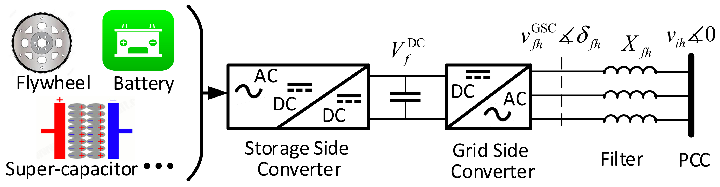This limitation is set as the maximum value of available power of the ESS (P^max–P_et,1) for idle periods and allowable 10% variation in output power (P_et,1) for charging or discharging periods. This constraint is mathematically shown as the maximum value of these two values in Equation (16). Furthermore, with respect to the general model of AHF as shown in Figure 4, working constraints could be formulated as Equations (17) and (18). In harmonic studies, harmonic voltages and currents are superimposed to the fundamental voltage and current. Hence, voltage and currents should be replaced with harmonic root mean square equivalents, as shown in Equations (17) and (18). The maximum current of AHF is limited to the maximum value, I^max in Equation (17). In Equation (18), the maximum allowable limit of AHF is considered as V^max.

$$d_{ft}^2=V_{ft,1}^2{\displaystyle \sum _{h>1}{i}_{fht}^2}\le {\left(D_{ft}^{\max }\right)}^2$$

(15)

$$D_{ft}^{\max }=\max \left\{P_e^{\max }-P_{et,1},10\%\left(P_{et,1}\right)\right\},\hspace{1em}\forall f\in ESS$$

(16)

$$I_{ft,1}^2+{\displaystyle \sum _{h>1}{i}_{fht}^2}\le {\left(I_f^{\max }\right)}^2,\hspace{1em}\forall f$$

(17)

$$V_{ft,1}^2+{\displaystyle \sum _{h>1}{v}_{fht}^2}\le {\left(V_f^{\max }\right)}^2,\hspace{1em}\forall f$$

(18)

The SOC of the ESS should also be taken into account in harmonic conditions. Although harmonic power transactions have low values, their effects on the SOC of the ESS should be considered. Harmonic active power (p_fth) can be calculated using the real value of the product of harmonic voltage and current as shown in Equation (19). The SOC of the ESS should be modified with respect to the provided active harmonic power. Since the PE converter of the ESS is generally a four-quadrant converter, harmonic active powers could be positive and negative. This could lead the ESS to be charged or discharged to provide the harmonic compensation current. Variations in the SOC in harmonic condition (c_fth) with respect to the provided active harming powers is mathematically shown in Equation (20). In Equation (20), the SOC in the harmonic condition is supposed to be equal to the SOC for fundamental frequency (C_ft) plus harmonic active powers, p_fth. Harmonic reactive power is usually achieved by changing the phase angle and modulation method of the converter. It can be considered as extra losses of active power and is usually considered as a percentage of active harmonic power [36]. This modification could be applied in Equation (20), which could be a subject for future research. Finally, the minimum and maximum limitations of the SOC should also be met in harmonic activities, which is mathematically shown in Equation (21).

$$p_{fth}=\mathrm{Re}\left\{v_{ith}{i}_{ith}^{\ast }\right\},\hspace{1em}\forall i\in {\mathsf{\Omega }}^{\mathrm{ESS}}$$

(19)

$$c_{fth}=C_{ft}+{\displaystyle {\sum }_{h>1}{p}_{fth}},\hspace{1em}\forall f\in \mathrm{ESS}$$

(20)

$$C_f^{\min }\le c_{fth}\le C_f^{\max },\hspace{1em}\forall f\in \mathrm{ESS}$$

(21)

Harmonic standards are usually reported as total harmonic distortion (THD) and individual harmonic distortion (IHD). Typical levels of harmonic standards for grid voltage are 5% and 3% for THD and IHD, respectively [37]. The important goal of the MG operator is the economic satisfaction of the desired harmonic levels across the entirety of the MG at each period. These constraints are shown in Equations (22)–(23), respectively, for THD and IHD. In each operation period, the THD could be met for each bus and the IHD should be met for each bus in each harmonic order.

$${\displaystyle {\sum }_{h>1}{v}_{ith}^2}\le {\left|V_{ih,1}\right|}^2{\left({\mathrm{THD}}_i^{\max }\right)}^2,\hspace{1em}\forall i,t$$

(22)

$$v_{ith}^2\le {\left|V_{it,1}\right|}^2{\left({\mathrm{IHD}}_i^{\max }\right)}^2,\hspace{1em}\forall i,\forall t,\forall h$$

(23)

The harmonic power flow constraints should also be considered in the model. Since the provided harmonic current compensation is injected to the MG in different nodes, these constraints are essential for calculations of the flow of harmonic powers. The constraints of Equations (24) and (25) are the harmonic counterparts of fundamental power flow previously shown in Equations (12) and (13). Furthermore, the harmonic spectrum approach is used for the harmonic modeling of nonlinear loads [33]. It is required to determine the magnitude and phase angle of harmonic injections of nonlinear loads in this approach. In Equation (26), the magnitude of harmonic injection (i_iht) is determined based on the harmonic spectrum of nonlinear load (I^spec) and current injection of the load in the fundamental frequency (I_it,1) for all buses of the network with nonlinear load (Ω^NL). The phase angle of harmonic injection (θ_ith) was also determined in Equation (27) using the phase spectrum of the nonlinear load (θ^spec) and the phase angle of its current injection in the fundamental frequency (θ_it,1).

$$\left[U_h\right]=\left[A_h\right]\left[I_h\right]$$

(24)

$$\left[\Delta V_h\right]={\left[B_h\right]}^T\left[Z_h\right]\left[U_h\right]$$

(25)

$$i_{iht}=I_{iht}^{\mathrm{spec}}\times I_{it,1},\hspace{1em}i\in {\mathsf{\Omega }}^{\mathrm{NL}}$$

(26)

$${\theta }_{ith}={\theta }_{ith}^{\mathrm{spec}}+h{\theta }_{it,1}+\pi ,\hspace{1em}i\in {\mathsf{\Omega }}^{\mathrm{NL}}$$

(27)

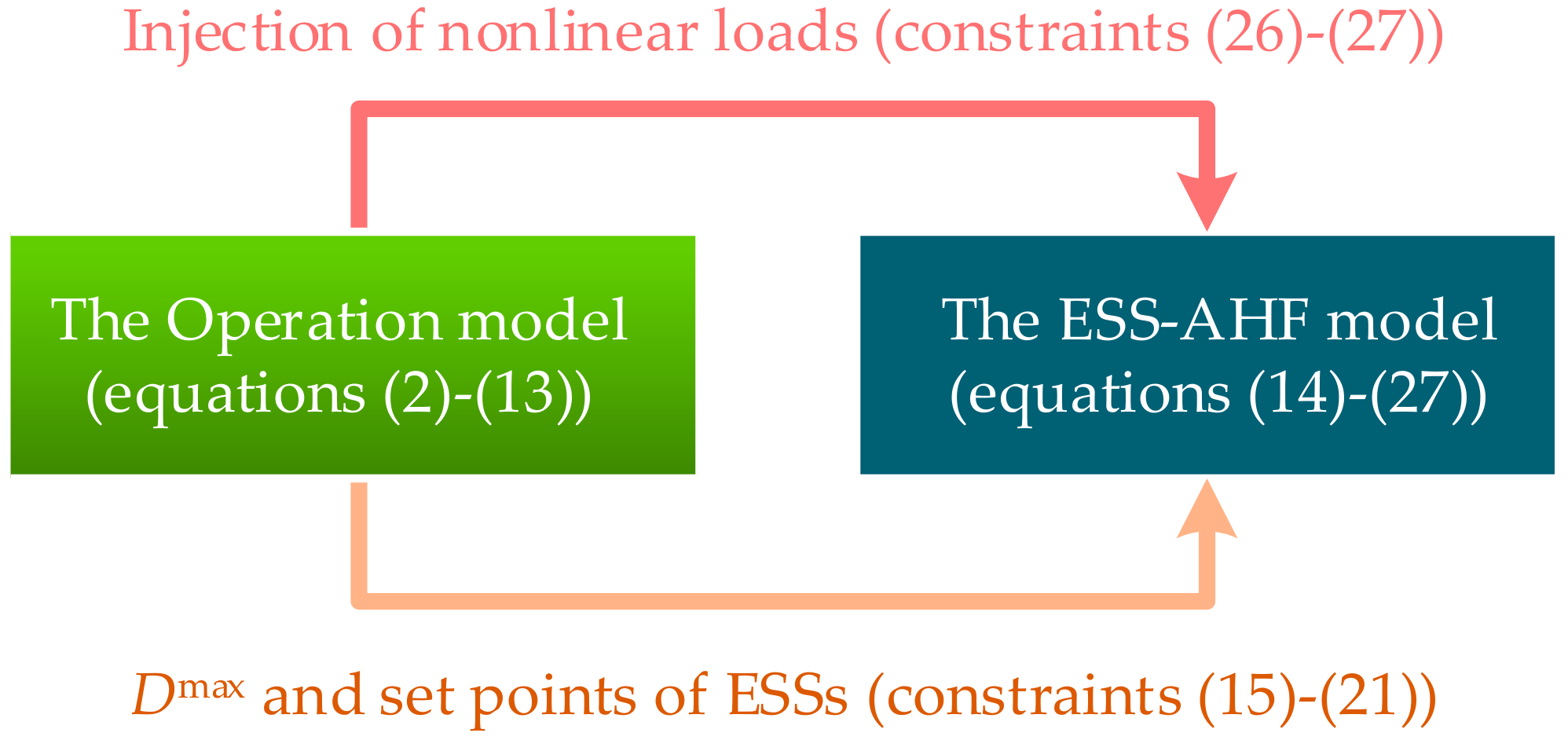
The developed model in Equations (14)–(27) is the complete model proposed for the coordinated operation of ESSs working as AHFs. It should be noted that the operation model of Equations (2)–(13) and the ESS-AHF model of Equations (14)–(27) are related and the ESS-AHF model will be implemented after the operation model. Hence, the ESS-AHF model could be accounted for as a sequential model, as shown in Figure 5. The output nonlinear load current of the operation model is the setpoints for the calculation of harmonic injections. These dependencies are mathematically shown in Equations (26) and (27). Harmonic injections are calculated in Equations (26) and (27) based on the harmonic spectrum of the nonlinear load. Hence, these dependencies could affect the ESS-AHF model since the harmonics will be related to harmonic injections of nonlinear loads. Furthermore, since ESSs are employed as AHFs in addition to APLCs, the working conditions of ESSs could be affected by the output of the operation model. The maximum available capacity of the distortion power for ESSs is set as the maximum value of available power of the ESS and allowable 10% variation in output power for charging or discharging periods, as shown in Equation (16). Hence, these setpoints could change the ESS activities as AHFs.

The output of the ESS-AHF model is the calculated harmonic reference currents of the ESSs, which should be injected into the MG. These reference currents are then transmitted to the ESSs by the available infrastructures of the MG, and the AHF works in the current control mode. Various technical constraints, harmonic conditions of the network, and the status of AHFs should be sent to the MG control center for consideration in the optimization problem. All of these require a proper communication infrastructure that could be available in future MGs. The availability of communication links in AHF buses, its bandwidth, and time delay are important challenges of the communication system that could affect the applicability of the proposed optimization method, which should be taken into account in future studies. In the next section, the results of the implementation of the proposed model will be represented.

5. Simulations

A modified version of the IEEE 33-bus test network was used to demonstrate the performance of the ESS-AHF model. The test grid consists of 32 branches and five tie-switches, as shown in Figure 6. Line and bus data were taken from [38] and are provided in Appendix A. In order to increase the effects of harmonics, line impedances were increased by a factor of three. Data for the daily load demand were taken from [39].

Four nonlinear loads were connected to the test network. The locations and active and reactive powers of nonlinear loads are shown in

Table 1. Nonlinear loads of the network.

Nonlinear Load	Bus	P (pu)	Q (pu)
1	14	0.150	0.120
2	20	0.125	0.105
3	23	0.110	0.100
4	30	0.145	0.125

. A general non-linear load model as a six-pulse diode bridge rectifier was adopted for all nonlinear loads [33]. The represented harmonic loads are the main sources of harmonic distortions in the MG. The harmonic spectrum of nonlinear loads is reported in

Table 2. Harmonic spectrum of nonlinear loads.

Harmonic	Magnitude	Phase (°)
5	0.35	180
7	0.43	180
11	0.05	0
13	0.08	0
17	0.04	180
19	0.04	180

, where the data were taken from [33]. In the harmonic spectrum approach, the magnitude and phase of the harmonic injections of nonlinear loads are used to calculate the flow of harmonic power in the network individually at each harmonic frequency.

Five DERs were added to the test network in selected buses, as shown in Figure 6. A parking lot of electric vehicles was considered at bus #12, a wind turbine was installed at bus #21, a photovoltaic (PV) generator was installed at bus #24, a battery energy storage was connected at bus #28, and finally, a PV array was connected at bus #31 equipped with a battery energy storage. The parking lot at bus #12 included a battery ESS. Hence, three ESSs have been placed in the test network which could be used as possible AHFs. Furthermore, two APLCs were connected to the network in buses #2 and #9, as shown in Figure 6. Hence, the total number of AHFs was equal to five filters. Data of the DER and APLCs are presented in

Table 3. Data of APLCs and DER of the network (values are in pu).

No	ID	Type	Bus	Smax	Imax	Cmin	Cmax	Pmax	π ($/kVARh)
1	APLC #1	APLC	2	0.22	0.43	---	---	0.32	860
2	APLC #2	APLC	9	0.18	0.35	---	---	0.26	900
3	ESS #1	Electric vehicle + ESS	12	0.1	0.1	0.1	0.25	0.1	395
4	DG #1	Wind turbine	21	0.15	0.15	---	---	0.15	---
5	DG #2	Photovoltaic	24	0.08	0.1	---	---	0.08	---
6	ESS #2	Battery storage	28	0.15	0.25	0.15	0.50	0.15	380
7	ESS #3	Photovoltaic + ESS	31	0.1	0.35	0.1	0.22	0.1	380

. The maximum and minimum of the SOC and maximum power of each ESS are also reported in this table. In the last column, the offered price of distortion power is shown based on $/kVARh. The offered prices for ESSs were lower than the APLCs since harmonic filtering is considered as a side function from ESSs, which leads to a reduced distortion power cost.

The lower and upper bounds of voltage were taken as 0.95 pu and 1.05 pu, respectively. The operation horizon for unit commitment problem is considered the next day, which is divided into hourly periods. The proposed optimization models (in the form of a mixed-integer nonlinear programming model) were implemented in GAMS software (GAMS Development Corporation, Washington, D.C., USA) [40] in a personal computer equipped with a 2.93 GHz Intel processor and 8 GB memory. Without loss of generality, it was assumed that the MG works in grid-connected mode. Hence, the voltage at the PCC is assumed to be sinusoidal.

Three different cases were considered to show the performance of the ESS-AHF model.

• Case I: ESSs are only used for energy arbitrage to reduce the cost of supplying energy to the customers.
• Case II: Employing APLCs for harmonic compensation imposed by nonlinear loads.
• Case III: Employing ESSs as AHFs to satisfy harmonic standards.

The simulation results are reported in the following three subsections.

5.1. Case I: The Base Case

In the base case, the unit commitment model of 4.1 was implemented on the test network. The various cost terms after running the model are summarized in

Table 4. Operation cost for the test network in Case I.

Total OC (k$)	Grid Cost (k$)	DG Cost (k$)		ESS Cost (k$)
2410	2104	248		58
		DG #1	DG #2	ESS #1	ESS #2	ESS #3
		86.4	161.6	17	28	13

. The total OC was equal to 2410 k$, 87% of which was due to the energy supplied by the main grid. The other 13% of the OC was due to the energy produced or exchanged by DGs and ESSs. The cost of the energy supplied by DGs was equal to 248 k$ and represented the revenue of DG owners for participating in the energy market. In the revenue of DG #2, the PV at bus #24 was higher compared to other DERs for its proper location. Moreover, smart charging and discharging of ESSs implied a revenue of 58 k$ from energy arbitrage. This revenue is, of course, a cost for the MG operator. In particular, ESS #2, the battery storage at bus #28, earnt about 50% of the total ESSs revenues.

The charging profile as well as the SOC of ESSs in the operation horizon is shown in Figure 7. All ESSs were charged from 3 am to 6 am, which are the off-peak periods of the operation horizon. Similarly, ESSs are discharged in peak periods from 5 pm to 7 pm. In Figure 7b, the SOCs of ESSs are represented. Allowable limits in Table 4 for the SOC and maximum power are met by the optimization model. Variation of the SOC for ESS #2 with more energy capacity at off-peak and peak periods can be seen in this figure.

However, the harmonic conditions should also be considered for PQ monitoring of the MG. In Figure 8, the voltage THD of the MG was analyzed. The voltage THD of all buses at 5 am (as the lowest) and 6 pm (as the highest load demand), are shown in Figure 8a. Obviously, either for off-peak periods or peak periods, the THD was above the standard level for nearly all system buses. All other periods may have a THD trend between these two selected periods. Bus #17 had the maximum THD compared to other buses. In Figure 8b, the voltage THD of this bus was represented in the operation horizon. The standard THD level is never met and hence, compensation actions are necessary.

In order to mitigate the harmonics effects from the grid, two simulation cases are provided to show the performance of the ESS-AHF model.

5.2. Case II: Harmonic Compensation Using APLCs

In Case II, only APLCs were employed for harmonic mitigation. APLCs were placed in the network based on filtering requirements and economic conditions by optimization models. The voltage THD of the system buses and the maximum THD after compensation of the APLCs are shown in Figure 9 for this case. Although the harmonic pollution was improved when compared to Case I, it was still above the standard level of 5%. This situation is worthwhile in peak periods, as shown in Figure 9a, since harmonic injections of nonlinear loads are increased in these periods. The maximum THD was for bus #32, which was about 11%. In Figure 9b, the maximum THD is shown for this bus. For off-peak periods, APLCs could adjust the voltage THD at the standard level. However, most of the time, the voltage THD is high, which could be the result of insufficient harmonic filtering capacity in the MG.

In Figure 10 the loading of each APLC is shown for Case II. In almost all periods (except off-peak ones), the APLCs were loaded at their maximum rating. However, they could not satisfy the harmonic standard in the MG. Hence, more harmonic filters are required to be employed for more filtering capacity in the MG. This could be achieved using more APLCs. However, it seems that this is not an economic solution. With respect to the high investment costs of the APLCs, it could significantly increase the cost of PQ compensation actions.

In the next case, the performance of ESSs for improving the harmonic situation of the MG as an economical alternative to APLCs is presented.

5.3. Case III: Harmonic Compensation Using ESSs

In order to increase the harmonic filtering capability of the MG as well as reduce the costs of PQ improvement actions, ESSs are also employed in this case for harmonic compensation. To this end, the unloaded power capacity of ESSs is used for harmonic filtering activities. Even if the ESS does not contribute to energy arbitrage, it can provide harmonic filtering capacity for the network. The results of the implementation of the ESS-AHF model are represented in this subsection.

The voltage THD and the maximum THD at each hour are represented in Figure 11. As it could be seen, the maximum THD in all periods of the operation horizon was adjusted at the standard level. For either the off-peak periods or peak periods, the voltage THD was in the acceptable range. Hence, using ESSs as AHFs has provided more harmonic filtering capacity for the MG. Furthermore, since the ESSs are dispersed in the MG, the provided compensation currents could be considered as distributed harmonic compensation actions. In this scheme, harmonic compensation currents are injected in the grid, and hence harmonic propagation and the resulting losses are strongly reduced. In Figure 13b, the maximum THD of voltage buses is shown, which was adjusted to the 5% standard level. This shows the effects of ESSs for the adjustment of harmonic standards for MGs.

The loadings of various AHFs are shown in Figure 12 for Case III. AHFs based on ESSs are almost loaded at their maximum capacity. This is the result of their lower prices for compensation distortion power as well as their location. Since the APLCs have expensive distortion power, their compensation loadings are performed after ESSs and generally have lower values compared to ESSs. APLC #2 had more compensation loading despite its higher cost. This shows the effects of filter location on its provided harmonic compensation to the MG.

The harmonic active power and the SOC of ESSs after harmonic compensation activities are reported in Figure 13. The provided harmonic active power was negative for all ESSs, which shows that it worked in discharging mode for harmonic compensation. However, the harmonic injection powers had low values compared to the fundamental active power previously shown in Figure 7. This means that participating in harmonic compensation activities does not have a significant effect on the SOC of ESSs, which can be seen Figure 13b. The trend of the SOC was close to the trend of that in Figure 7 and all allowable limits were met in the harmonic conditions. Hence, the harmonic utilization of ESSs could bring various advantages for the MG, and meanwhile, does not affect the ESS parameters for energy arbitrage. The ESSs earn from both energy arbitrage and harmonic compensation.

The required reference currents of the ESSs at each period are determined in the ESS-AHF model. Fundamental harmonic and reference currents for ESS #2 at the peak period (i.e., 6 pm) are shown in Figure 14. The bold curve is the required reference current calculated by the ESS-AHF model, which should be injected by the ESS. The reference current should then be sent to the ESS by the available infrastructures of the MG. The ESS is responsible to inject the required current by the MG operator with a suitable control and switching method.

For economic comparisons, the total injections and compensation costs for Case III are presented in

Table 5. Total harmonic compensation injection of AHF in Case II and Case III.

ID		APLC #1	APLC #2	ESS #1	ESS #2	ESS #3	Total
Case II	Injection (pu)	4.63	4.32	0	0	0	8.95
	Cost ($)	3980	3888	0	0	0	7868
Case III	Injection (pu)	0.16	1.79	1.74	1.29	1.31	6.29
	Cost ($)	140	1607	689	491	497	3424

. The total required distortion power was 8.95 pu and 6.29 for Case II and Case III, respectively. Although the compensation distortion power in Case III was about 70% of that in Case II, it could successfully meet the desired level of harmonics in the MG, as shown in Table 5. Furthermore, the loading of compensation currents was more achieved by the ESSs in Case III as they were more economic AHFs compared to the APLCs. This reduces the total compensation cost from 7868 k$ in Case II to 3424 k$ in Case II. It showed a 44% decrease in the compensation cost. Hence, the MG operator could keep the desired harmonic level with only 44% of the cost of the APLCs. This could save remarkable costs for the MG operator, either in the operation of the APLCs or as requirements for the installation of new APLCs.

The simulations showed the performance of the ESS-AHF model in the coordination of distributed ESSs for harmonic compensation in the MG. More filtering capacity and reduced compensation costs are the main advantages of ESSs in harmonic compensation. Since harmonic compensation is utilized as a side function, the provided distortion power has a lower price than APLCs. This implies that compensation loading is first demanded by the ESSs. Furthermore, ESSs are dispersed in the MG, and hence harmonic compensation will be distributed in the MG. The provided compensation scheme will be accounted for by distributed harmonic compensation with more flexibility and applicability for PQ improvements. The ESS owners could also benefit from both energy arbitrage and harmonic compensation. This could decrease the investment costs of the ESSs and make them more justified for use in the MG. The simulations showed that ESS compensation activities do not have much of an effect on the SOC and ESS revenues from energy arbitrage. Finally, it should be noted that, unlike energy and ancillary markets, PQ improvement actions are not security obligations of the network. Therefore, any time that the working of ESSs in PQ improvement actions affects their application in ancillary services and the security of the network, it could be temporarily ignored.

6. Conclusions

In this paper, the applicability of ESSs for harmonic filtering activities was investigated. The common procedure for this was to modify the control methods of the PE converters of ESSs to enable them for the injection of compensation currents. However, in this paper, the coordinated operation of ESSs for a distributed harmonic compensation scheme was addressed. The proposed coordination model employed conventional control algorithms for the injection of a reference current that was determined in the proposed ESS-AHF optimization model. Hence, the provided compensation scheme could be considered as a distribution compensation scheme. The simulation cases showed the performance of the proposed model in enhancing the filtering capability of the MG, the reduction in compensation cost, and the greater flexibility of the distributed compensation schemes. Hence, requirements for new filters could be deferred and both the MG operator and the ESS owner could benefit from reduced compensation costs.

ESSs can be used to perform several ancillary services where most of them need the energy stored to be accomplished. What is demonstrated in this paper is that the ancillary service for harmonic power filtering can be performed without significantly affecting the battery SOC. For this reason, this service can be achieved for free, without compromising the others, and therefore the revenues from energy arbitrage and other ancillary services can be maintained. This could make ESSs more economical for use in future power systems. Investigations should be carried out for various technical and systematic challenges of the proposed ESS-AHF model in future research.

References

1. Koohi-Kamali, S.; Tyagi, V.; Rahim, N.; Panwar, N.; Mokhlis, H. Emergence of energy storage technologies as the solution for reliable operation of smart power systems: A review. Renew. Sustain. Energy Rev. 2013, 25, 135–165. [Google Scholar] [CrossRef]
2. Zakeri, B.; Syri, S. Electrical energy storage systems: A comparative life cycle cost analysis. Renew. Sustain. Energy Rev. 2015, 42, 569–596. [Google Scholar] [CrossRef]
3. Luo, X.; Wang, J.; Dooner, M.; Clarke, J. Overview of current development in electrical energy storage technologies and the application potential in power system operation. Appl. Energy 2015, 137, 511–536. [Google Scholar] [CrossRef] [Green Version]
4. Kondoh, J.; Ishii, I.; Yamaguchi, H.; Murata, A.; Otani, K.; Sakuta, K.; Higuchi, N.; Sekine, S.; Kamimoto, M. Electrical energy storage systems for energy networks. Energy Convers. Manag. 2000, 41, 1863–1874. [Google Scholar] [CrossRef]
5. Marini, A.; Ghazizadeh, M.-S.; Mortazavi, S.S.; Piegari, L. A harmonic power market framework for compensation management of DER based active power filters in microgrids. Int. J. Electr. Power Energy Syst. 2019, 113, 916–931. [Google Scholar] [CrossRef]
6. Beleiu, H.; Beleiu, I.; Pavel, S.; Darab, C. Management of Power Quality Issues from an Economic Point of View. Sustainability 2018, 10, 2326. [Google Scholar] [CrossRef] [Green Version]
7. Das, C.K.; Bass, O.; Kothapalli, G.; Mahmoud, T.S.; Habibi, D. Overview of energy storage systems in distribution networks: Placement, sizing, operation, and power quality. Renew. Sustain. Energy Rev. 2018, 91, 1205–1230. [Google Scholar] [CrossRef]
8. Buła, D.; Lewandowski, M. Comparison of frequency domain and time domain model of a distributed power supplying system with active power filters (APFs). Appl. Math. Comput. 2014, 267, 771–779. [Google Scholar] [CrossRef]
9. Kalair, A.; Abas, N.; Kalair, A.; Saleem, Z.; Khan, N. Review of harmonic analysis, modeling and mitigation techniques. Renew. Sustain. Energy Rev. 2017, 78, 1152–1187. [Google Scholar] [CrossRef]
10. Mohamad, F.; Teh, J.; Lai, C.-M.; Chen, L.-R. Development of energy storage systems for power network reliability: A review. Energies 2018, 11, 2278. [Google Scholar] [CrossRef] [Green Version]
11. Alshehri, J.; Khalid, M.; Alzahrani, A. An Intelligent Battery Energy Storage-Based Controller for Power Quality Improvement in Microgrids. Energies 2019, 12, 2112. [Google Scholar] [CrossRef] [Green Version]
12. Khani, H.; Farag, H.E. Optimal scheduling of energy storage to mitigate power quality issues in power systems. In Proceedings of the 2017 IEEE Power & Energy Society General Meeting, Chicago, IL, USA, 16–20 July 2017; pp. 1–5. [Google Scholar]
13. Ramos, G.; Rios, M.; Gómez, D.; Palacios, H.; Posada, L. Power quality study of large-scale wind farm with battery energy storage system. In Proceedings of the 2017 IEEE Industry Applications Society Annual Meeting, Cincinnati, OH, USA, 1–5 October 2017; pp. 1–6. [Google Scholar]
14. Yang, D. Informatics in Control, Automation and Robotics; Springer: Berlin/Heidelberg, Germany, 2012; Volume 2. [Google Scholar]
15. Arulampalam, A.; Barnes, M.; Jenkins, N.; Ekanayake, J.B. Power quality and stability improvement of a wind farm using STATCOM supported with hybrid battery energy storage. IEE Proc. Gener. Transm. Distrib. 2006, 153, 701–710. [Google Scholar] [CrossRef]
16. Marini, A.; Piegari, L.; Mortazavi, S.S.; Ghazizadeh, M.-S. Active Power Filter Commitment for Harmonic Compensation in Microgrids. In Proceedings of the 45th Annual Conference of the IEEE Industrial Electronics Society, IECON 2019, Lisbon, Portugal, 14–17 September 2019; pp. 7038–7044. [Google Scholar]
17. Das, J. Power System Harmonics and Passive Filter Designs; John Wiley & Sons: Hoboken, NJ, USA, 2015. [Google Scholar]
18. Abolhassani, M.T.; Enjeti, P.; Toliyat, H. Integrated doubly fed electric alternator/active filter (IDEA), a viable power quality solution, for wind energy conversion systems. IEEE Trans. Energy Convers. 2008, 23, 642–650. [Google Scholar] [CrossRef]
19. Abolhassani, M.T.; Enjeti, P.; Toliyat, H.A. Integrated doubly-fed electric alternator/active filter (IDEA), a viable power quality solution, for wind energy conversion systems. In Proceedings of the Conference Record of the 2004 IEEE Industry Applications Conference, 2004. 39th IAS Annual Meeting, Seattle, WA, USA, 3–7 October 2004; Volume 2033, pp. 2036–2043. [Google Scholar]
20. Ghatpande, O.A. Harmonic Compensation in A Grid Using Doubly Fed Induction Genertors. Master’s Thesis, Missouri University of Science and Technology, Rolla, MO, USA, 2013. [Google Scholar]
21. Naidu, N.S.; Singh, B. Doubly fed induction generator for wind energy conversion systems with integrated active filter capabilities. IEEE Trans. Ind. Inform. 2015, 11, 923–933. [Google Scholar] [CrossRef]
22. Ying-Kwun, C. Determination of locations and sizes for active power line conditioners to reduce harmonics in power systems. IEEE Trans. Power Deliv. 1996, 11, 1610–1617. [Google Scholar] [CrossRef]
23. Hong, Y.-Y.; Hsu, Y.-L.; Chen, Y.-T. Three-phase active power line conditioner planning. In Generation, Transmission and Distribution, IEE Proceedings. IET 1998, 145, 281–287. [Google Scholar]
24. Alfonso, J.L.; Gonçalves, H.; Pinto, J. Active Power Conditioners to Mitigate Power Quality Problems in Industrial Facilities; IntechOpen Publisher: London, UK, 17 April 2013; Open Access. [Google Scholar]
25. Griffo, A.; Carpinelli, G.; Lauria, D.; Russo, A. An optimal control strategy for power quality enhancement in a competitive environment. Int. J. Electr. Power Energy Syst. 2007, 29, 514–525. [Google Scholar] [CrossRef] [Green Version]
26. Mortezaei, A.; Simoes, M.; Savaghebi, M.; Guerrero, J.; Al-Durra, A. Cooperative control of multi-master-slave islanded microgrid with power quality enhancement based on conservative power theory. IEEE Trans. Smart Grid 2016, 99, 1. [Google Scholar]
27. Wasiak, I.; Pawelek, R.; Mienski, R. Energy storage application in low-voltage microgrids for energy management and power quality improvement. IET Gener. Transm. Distrib. 2013, 8, 463–472. [Google Scholar] [CrossRef]
28. Cespedes, M.; Sun, J. Impedance modeling and analysis of grid-connected voltage-source converters. IEEE Trans. Power Electron. 2014, 29, 1254–1261. [Google Scholar] [CrossRef]
29. Cao, W.; Ma, Y.; Zhang, X.; Wang, F. Sequence impedance measurement of three-phase inverters using a parallel structure. In Proceedings of the Applied Power Electronics Conference and Exposition (APEC), Charlotte, NC, USA, 15–19 March 2015; pp. 3031–3038. [Google Scholar]
30. Cao, W. Impedance-Based Stability Analysis and Controller Design of Three-Phase Inverter-Based Ac Systems. Ph.D. Thesis, University of Tennessee, Knoxville, TN, USA, 2017. [Google Scholar]
31. Marini, A.; Mortazavi, S.; Piegari, L.; Ghazizadeh, M.-S. An efficient graph-based power flow algorithm for electrical distribution systems with a comprehensive modeling of distributed generations. Electr. Power Syst. Res. 2019, 170, 229–243. [Google Scholar] [CrossRef]
32. Farhoodnea, M.; Mohamed, A.; Shareef, H.; Zayandehroodi, H. Optimum placement of active power conditioner in distribution systems using improved discrete firefly algorithm for power quality enhancement. Appl. Soft Comput. 2014, 23, 249–258. [Google Scholar] [CrossRef]
33. Grady, W.M.; Santoso, S. Understanding power system harmonics. IEEE Power Eng. Rev. 2001, 21, 8–11. [Google Scholar] [CrossRef]
34. Marini, A.; Latify, M.A.; Ghazizadeh, M.S.; Salemnia, A. Long-term chronological load modeling in power system studies with energy storage systems. Appl. Energy 2015, 156, 436–448. [Google Scholar] [CrossRef]
35. Marini, A.; Latify, M.-A.; Ghazizadeh, M.-S.; Salemnia, A. Joint Maintenance Scheduling of Generation Units and Energy Storage Systems. Tabriz J. Electr. Eng. 2017, 46, 78. [Google Scholar]
36. Farahani, H.F.; Shayanfar, H.; Ghazizadeh, M. Modeling of stochastic behavior of plug-in hybrid electric vehicle in a reactive power market. Electr. Eng. 2014, 96, 1–13. [Google Scholar] [CrossRef]
37. IEEE Recommended Practice for Monitoring Electric Power Quality; IEEE Std 1159–2009 (Revis. IEEE Std 1159–1995); IEEE: Piscataway, NJ, USA, 2009; pp. 1–81. [CrossRef]
38. Abbas Marini, L.P.S.S.; Mortazavi, M.S. Ghazizadeh. In A linear programming approach to distribution Power Flow. In Proceedings of the 6th International Conference on Clean Electrical Power (ICCEP), Santa Margherita, Italy, 27–29 June 2017. [Google Scholar]
39. Barrows, C.; Bloom, A.; Ehlen, A.; Ikaheimo, J.; Jorgenson, J.; Krishnamurthy, D.; Lau, J.; McBennett, B.; O’Connell, M.; Preston, E. The IEEE reliability test system: A proposed 2019 Update. IEEE Trans. Power Syst. 2019, 99, 1. [Google Scholar] [CrossRef]
40. Rosenthal, E. GAMS-A user’s guide. In Proceedings of the GAMS Development Corporation, Washington, DC, USA, 1–13 May 2008. [Google Scholar]
Figure 1. Schematics of the shunt and series active harmonic filters.
Energies 13 00771 g001
Figure 2. Output power and duration of various ESSs (plot obtained with data taken from [4]).
Energies 13 00771 g002
Figure 3. General connection of the ESSs by a voltage source inverter to the PCC.
Energies 13 00771 g003
Figure 4. Harmonic model of ESSs in harmonic compensation.
Energies 13 00771 g004
Figure 5. The ESS-AHF model as a sequential model after the operation model.
Energies 13 00771 g005
Figure 6. Modified IEEE 33-bus test network.
Energies 13 00771 g006
Figure 7. Case I. (a) Charging profile and (b) the SOC of each ESS.
Energies 13 00771 g007
Figure 8. Case I. (a) Voltage THD for all buses at t = 5 and t = 18 and (b) maximum voltage THD of all buses at each hour.
Energies 13 00771 g008
Figure 9. Case II. (a) Voltage THD for all buses at t = 5 and t = 18 and (b) maximum voltage THD of all buses at each hour.
Energies 13 00771 g009
Figure 10. The loaded capacity of the APLCs for harmonic filtering in Case II.
Energies 13 00771 g010
Figure 11. Case III. (a) Voltage THD for all buses at t = 5 and t = 18 and (b) maximum voltage THD of all buses at each hour.
Energies 13 00771 g011
Figure 12. The loaded capacity of AHFs for harmonic filtering in Case III.
Energies 13 00771 g012
Figure 13. Case III. (a) Discharging profile and (b) the SOC of each ESS for harmonic compensation.
Energies 13 00771 g013
Figure 14. Fundamental harmonic and reference currents of ESS #2 in the peak period, (6 pm) in Case III.
Energies 13 00771 g014