Abstract
This work proposes a fault detection and imputation scheme for a fleet of small-scale photovoltaic (PV) systems, where the captured data includes unlabeled faults. On-site meteorological information, such as solar irradiance, is helpful for monitoring PV systems. However, collecting this type of weather data at every station is not feasible for a fleet owing to the limitation of installation costs. In this study, to monitor a PV fleet efficiently, neighboring PV generation profiles were utilized for fault detection and imputation, as well as solar irradiance. For fault detection from unlabeled raw PV data, K-means clustering was employed to detect abnormal patterns based on customized input features, which were extracted from the fleet PVs and weather data. When a profile was determined to have an abnormal pattern, imputation for the corresponding data was implemented using the subset of neighboring PV data clustered as normal. For evaluation, the effectiveness of neighboring PV information was investigated using the actual rooftop PV power generation data measured at several locations in the Gwangju Institute of Science and Technology (GIST) campus. The results indicate that neighboring PV profiles improve the fault detection capability and the imputation accuracy. For fault detection, clustering-based schemes provided error rates of 0.0126 and 0.0223, respectively, with and without neighboring PV data, whereas the conventional prediction-based approach showed an error rate of 0.0753. For imputation, estimation accuracy was significantly improved by leveraging the labels of fault detection in the proposed scheme, as much as 18.32% reduction in normalized root mean square error (NRMSE) compared with the conventional scheme without fault consideration.
1. Introduction
A photovoltaic (PV) power plant is one of the most renewable, sustainable, and eco-friendly setups for converting solar energy, which is the most abundant and freely available energy source, into electrical energy [1]. The contribution of solar energy to the total global energy supply has rapidly increased in recent decades with PV installation capacity growing to more than 500 GW by the end of 2018 [2,3]. However, PV systems are exposed to harsh working conditions owing to uncertain outdoor environments and their complex structure. In [4], it was reported that the annual losses in PV generation reached 18.9% under zero or shading faults. Improving the reliability of renewable energy generation by fault detection and diagnosis (FDD) and correcting faulty data is essential for maintaining the efficiency of PV generation [5]. In addition, reliable information is required to be applied for various power applications, e.g., energy scheduling [6] and energy forecasting [7,8], to guarantee safe and stable grid systems.
For utility planners and operators, it is essential to examine the power output variability [9] to aggregate the fleet of PV systems, which is defined as the number of individual PV systems spread out over a geographical area [10]. Several studies presented station-pair correlation analyses by introducing virtual networks. A correlation was observed between short-term irradiance variability as a function of diverse distance and time scale [11]. Similarly, the maximum output variability of a fleet of PV plants was estimated by using the clearness index [12]. A variability model was built in [13] to integrate a large amount of generated solar power into power systems. To integrate the fleet as a distributed power source, it should be managed by an intelligent monitoring system that can correct abnormal data via real-time fault diagnosis and power generation forecasts.
PV faults occur because of various reasons at different locations, such as a module, string, or any other spot related to the PV systems. Visual and thermal methods employed in PV fault detection can detect superficial problems, such as browning, soiling or snow, discoloration, delamination, and hot spots, using auxiliary measurements [14]. However, this requires expensive and complicated equipment [15]. In recent years, many studies have employed methods using electrical variables via a data-driven approach. The electrical signal approaches are mainly referred to as maximum power point tracking (MPPT) with I–V characteristic analysis and power loss analysis. They are usually utilized to distinguish an open circuit, short circuit, degradation or aging, and shading faults that may typically occur on the DC side of a PV array [16,17,18].
For data-driven methods, automatic fault detection approaches can be categorized into conventional modeling-based methods and methods that utilize intelligent machine learning [19]. For the former case, the model can be built with respect to the physical attributes from the PV module specification for simulation settings to compare the desired output with the measured output [20]. Conventional statistical detection methods have been primarily presented in previous studies [16,21,22,23,24,25]. The exponentially weighted moving average has been used to identify DC side faults by comparing the one-diode model and estimated MPPs [21,22]. Lower and upper limits were set when the ratio of the measured to the modeled AC power exceeds 3-sigma [22]. In [23], outlier detection rules were proposed in their statistical details: The 3-sigma rule, Hampel identifier, and Boxplot rule using a PV string current. A symbolic aggregate approximation (SAX) scheme was used to convert the voltage profile, prior to performing clustering and anomaly detection [24].
With the advent of artificial intelligence (AI), which can be applied to various domains, particularly suited to the nonlinear behavior of PV systems, numerous studies have exploited AI-based monitoring systems [26]. The common artificial neural network (ANN) is widely used either to predict PV generation behavior or as a fault detection module based on several electrical parameters [15,27,28,29,30,31]. In comparison with a conventional back-propagation network, a probabilistic neural network (PNN) uses a probability density function as the activation function; thus, it is less sensitive to noisy and erroneous samples [32,33,34]. Fault detection by a support vector machine (SVM) has been used in several studies because it has the ability to separate objects by finding an optimal hyperplane that maximizes the margin in both binary and multiclass problems [35,36,37]. The decision tree (DT) builds repetitive decision rules within if/else instructions, which is intuitive. The model can be implemented conveniently with a large dataset [35,38]. The random forest (RF) has been applied to improve multiclass classification accuracy and to generalize performance [19]. Fuzzy classifications based on a fuzzy inference system (FIS) were developed by constructing logic rules [29,39]. A kernel extreme learning machine was investigated owing to its fast learning speed and good generalization [40]. Particle swarm optimization-back-propagation (PSO-BP) has been shown to improve the convergence and prediction accuracy of fault diagnosis systems [41].
Most of the data-driven approaches involve a supervised learning-based fault detection system that assigns a label for binary PV states as either normal or abnormal or as multi-class for corresponding fault types in advance. The detection or classification model learns the complex and unrevealed relation between input attributes and predefined labels in the training phase, and then the model is tested to determine whether it can distinguish PV states properly for new inputs. However, these processes require human effort to manually assign labels, and it is not easy to visualize the trained model. Graph-based semi-supervised learning (GBSSL) was proposed to detect line-to-line and open circuit faults using a few labeled data [42]. In [20], five types of faults were classified based on a single diode model with five input vectors associated with IV characteristics, solar irradiance, and temperature. Gaussian-fuzzy C-means was conducted using the distribution of each cluster and faults were diagnosed through PNN based on previous cluster center information [33]. A fuzzy membership algorithm based on degrees of fault data and cluster centers has been proposed [43]. Density peak-based clustering has also been proposed [44]. The 3-sigma rule was applied to determine each cluster center using the normalized voltage and current at the MPPs. Similarly, the PV local outlier factor (PVLOF) was computed from the current of the PV array to identify the degree of faults [45]. A single diode model-based prediction was implemented, enabling the generation of the residual, which was applied to the one-class SVM by quantifying the dissimilarity between the normal and faulty features [46].
In this study, we propose a framework of two stages of self-fault detection and self-imputation in a fleet of PV systems using neighboring PV power generation units based on correlation analysis. Because insolation data is not available with sufficient geographical resolution, especially for a small-scale PV system [12,37], neighboring PV generation data in the same fleet can be used jointly with distanced weather data. Since daily PV generation captures generally include unidentified erroneous samples, faulty data candidates were first labeled in the proposed scheme by an unsupervised manner with several extracted features. K-means clustering was employed to find out fault data point in the daily PV power outputs obtained from all the sites in the fleet. When the profile was considered as an abnormal pattern, restoration was accomplished by the following imputation step. Imputation schemes were implemented by autoregressive (AR) and multiple regression models with optional neighboring PV data of normal candidates obtained from the previous clustering step. For evaluation, several types of fault patterns observed in actual PV power profiles were simultaneously injected into a single or multiple sites, and proposed schemes were tested without injection information.
The remainder of this paper is organized as follows: Section 2 describes the PV fleet power output relationship between distance and the correlation with actual data measured on campus. Section 3 proposes an efficient fault detection and imputation methods for use with a PV fleet. The simulation setup, including the injected fault pattern, is provided in Section 4. Section 5 details the detection and imputation results, and Section 6 concludes the paper.
2. PV Fleet Power Data Analysis
2.1. Materials
In this study, actual PV fleet data were utilized for analysis and simulation. Hourly power generation data were measured in rooftop solar installations from 13 buildings at the Gwangju Institute of Science and Technology (GIST) campus located in Gwangju, South Korea, as shown in Figure 1, with installation details given in Table 1. In this densely distributed PV fleet, only the facility management building (site 3) collects environmental information, such as ambient temperature, module temperature, slope solar irradiance, and horizontal solar irradiance. The data were collected in 2019 for approximately nine months. To investigate the influence of solar irradiance with respect to the distance between the weather station and PV installation, local environmental data retrieved from the nearest weather station provided by the Korea Meteorological Administration (KMA) website were used [47]. The weather data including local solar irradiance were recorded every hour, the same as for the PV data. We selected 159 days of PV power data from 13 sites without missing values for an overlapping period. The meteorological data were acquired at the site weather station (SWS). In addition, a local weather station (LWS), which was approximately 7 km away from the campus, was subsequently employed for the same time period.
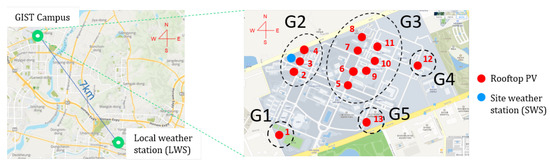
Figure 1.
Weather stations and photovoltaic (PV) fleet on the Gwangju Institute of Science and Technology (GIST) campus.

Table 1.
Installation information for rooftop PVs in the GIST fleet.
2.2. Cross-Correlation Analysis
Because previous studies have demonstrated that the correlation coefficient decreases when the distance between the weather station and the PV system increases, we investigated the cross-correlation as a function of distance. The cross-correlation is computed using the Pearson’s correlation coefficient as follows:
The covariance of two time-series data and , cov is normalized by the product of their standard deviation and . The correlation between each PV site with solar irradiance, which was obtained at SWS and LWS, was analyzed. As expected, the SWS data showed a stronger positive correlation than the LWS data for every site on the campus, as given in Table 2. The correlation analysis was conducted between PV generation data for each site in the same manner. Figure 2 shows the result of the correlation analysis, which produced five groups according to the degree of correlation. Apart from other sites, site 1 belonged to the independent group G1. Sites 2–4 were grouped into group 2 (G2) due to high correlation because of the relatively short distance from SWS. Group 3 (G3) comprised sites 5–11, which had a medium distance from SWS but were clustered together. Groups 4 (G4) and 5 (G5) comprised site 12 and 13, respectively, where one site was far from SWS and other sites. Based on the cross-correlation analysis, we determined that the use of neighbor PV power data can provide additional information that can help perform fault detection and imputation in the fleet of PV systems.
Table 2.
Cross-correlation of the PV power output between the local weather station (LWS) and the site weather station (SWS).
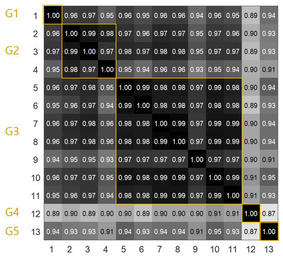
Figure 2.
Cross-correlation of PV power output for the fleet.
3. PV Fleet Fault Detection and Imputation
The overall scheme of the proposed system is shown in Figure 3. SWS data and 13 power output data sets from the PV fleet were provided, from which features were extracted to distinguish the daily binary condition of normal or faulty. At the clustering stage, daily states for each PV site were estimated, which is reflected by the final step of imputation.
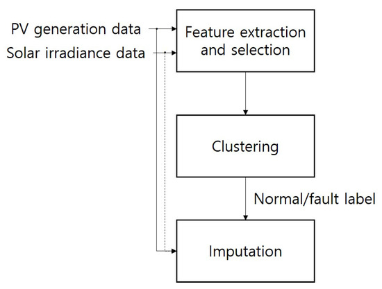
Figure 3.
Overall architecture of the proposed system.
3.1. Operation Time
Operation time was considered to extract meaningful properties from the PV pattern accordance with environmental factor. The daylight hours or insolation duration can be obtained by mathematical modeling based on geographical components, such as the latitude of the PV site, using the following equation:
where is the solar constant, which is 1368 [W/m2], d is the day number in the year, is the solar declination, is the latitude of the site, and is the solar hour angle. During an hour after sunrise and an hour before sunset, the small amount of solar irradiance has a tidal effect on PV operation. We defined the operation time, , by excluding these time periods from the insolation duration [37].
3.2. Feature Extraction
Several features were extracted from the given dataset (e.g., the PV fleet power data , and the solar irradiance observation data ) to distinguish the fault patterns from normal data at the candidate PV site n. In this study, as there is one SWS at site 3. We distinguished and , which represent the feature set derived from daily solar irradiance and daily neighboring PVs, respectively. Seven features were introduced in this study for two types of datasets, which generated 14 features. The extracted features of the candidate PV can be written as .
3.2.1. Total Coefficient of Determination
The coefficient of determination used in this study refers to how well a certain profile can explain the PV power generation profile for each PV site. For simulation comparison, the profile can be either solar irradiance data or neighboring PV generations, as follows:
where denotes the coefficients of determination of the regression depending on the other independent variable.
3.2.2. Normalized Profile Distance
The distance between normalized profiles is related to the closeness of the pattern shape. Daily profiles were converted within the range of [0,1] through min–max normalization, and the distance for each time step was computed, as follows:
where and .
3.2.3. Degree of Consistency
To investigate the fluctuation consistency, the degree of consistency between two profiles was proposed in [48]. Regardless of the heterogeneous dataset, e.g., comparing solar irradiance and PV generations or different capacities of the PV installations, it can reflect the variation tendency. During the operation time period, , , and count whether the variation tendency is identical, opposite, or zero, respectively. Then, they are converted into , , and to be computed as a ratio.
3.2.4. Relative Error Percentile of the Maximum Value
By comparing the relative maximum property of each profile, the relative error percentiles of the maximum values were determined. Two different attributes, i.e., the first order difference () and standard value (), were used:
where and .
where and .
3.3. Clustering
Because the condition of the PV system is not labeled in the real environment, unsupervised learning was applied in this study. K-means clustering is the simplest method and requires low computation based on calculation of the Euclidean distance. The objective function of K-means clustering, J, is given by Equation (10). Determining the number of clusters and importing the initial center have a crucial impact on the clustering accuracy. In our case, we set the number of clusters as two to distinguish between normal and fault patterns, and they were used in the imputation part for filtering the PV site candidates of the explanatory variables. Initial centroids were set to zero vectors and one vectors multiplied by 0.5 for the normal and fault condition, respectively. Optimal features were selected by exhaustive search for the objective function as follows:
where s is the number of clusters (, binary condition for the fault or normal state), is the center of cluster j, and are the selected features of site n. Feature selection results are shown in Section 5.
3.4. Imputation
Once the PV profile was labeled as a fault pattern, the fault data were restored using the regression method. In [49], the time series analysis of various meteorological data related to renewable energy systems was conducted using a statistical method. We built a linear regression model based on the linear minimum mean squared error (LMMSE) to estimate the regression parameter, as follows:
where P is the expected imputation profile at the candidate site, is the regression coefficient, X is the set of explanatory datasets, and is the random error.
In this study, several cases were studied to compare the explanatory dataset for the regression model and to investigate the impact of the labeling of neighboring PV profiles at the previous detection stage, as demonstrated in Table 3. In Case 1, we assumed that only PV historical power output data were available without any other measurements. In this case, we built an AR model for a single PV site to focus on its periodic power generation behavior. Case 2 exclusively considers local irradiance data. For our dataset, solar irradiance data provided at site 3 were used identically to construct the univariate simple regression model. Case 3 allows a neighbor PV profile that has unknown operation states in each PV system, and all of them are inputted into the multivariate regression model. Case 4 conducted a multiple regression model that was similar to Case 3 but the explanatory data were refined with the normal pattern classified at the previous detection stage. Case 5 merged Cases 2 and 4 that utilizes both local irradiance data and normal PV fleet data. Furthermore, as several previous works have confirmed that kNN is an efficient method for missing data imputation, we adopted kNN for fault data imputation as Case 6.
Table 3.
Imputation case study.
4. Simulations
4.1. Fault Pattern Injection
To evaluate the performance, we primarily sorted 159 days of PV generation patterns for all sites for the normal condition simultaneously. The overall normal dataset comprised PV power profiles. To characterize the fault patterns, the actual fault patterns detected from different PV plants were investigated. Six fault patterns were extracted, which were composed of whole zero, part zero, whole shift, part shift, constant padding, and spike, as shown in Figure 4. The faults were injected arbitrarily into a single or multiple power profiles of PV sites, thus retaining target labels to describe the performances of fault detection and imputation.
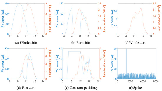
Figure 4.
Fault pattern for the actual observation.
4.2. Evaluation Metric
4.2.1. Fault Detection Performance Metric
A confusion matrix is widely used to evaluate classification performance, as depicted in Table 4. It matches the output label and target label for testing samples one by one; thus, target output label sets are sorted as true positive (TP), false negative (FN), false positive (FP), and true negative (TN). Based on these attributes, accuracy is derived as the ratio of correctly classified samples among all samples. The error rate is the opposite of accuracy, which indicates the error proportion for all samples. Precision is the ratio of TPs for all positives that are categorized in the test phase. Lastly, recall indicates the ratio of TPs out of all pre-labeled positives, as follows:
Table 4.
Confusion matrix.
4.2.2. Imputation Performance Metric
To evaluate the accuracy of imputation performance, normalized root mean square error (NRMSE) is adopted since the PV capacities in the fleet are different. In this study, RMSE was normalized by mean as described in Equations (14) and (15) Low NRMSE implies valuable imputation performance where abnormal pattern is restored similar to the real profile. The daily abnormal pattern for a corresponding site is then substituted by the reconstructed normal pattern.
where is the mean of during operation hours.
5. Results and Discussion
5.1. Feature Selection
The feature characterized in Section 3.2 can be assembled in various combinations. To determine the optimal parameter combination, an exhaustive search was followed by division into two scenarios: In one, combinations from were selected and the other involved . Table 5 and Table 6 list the detection performance for all datasets that included 2067 feature sets and labels with and without neighboring PV data, respectively. Accuracy, error rate, precision, and recall for all the combinations were surveyed. We selected high accuracy with a similar portion of false alarm and missing fault to increase detection accuracy and prevent inclination to one side. Features 1, 2, and 5 were selected from in the first scenario. However, the combination of features 1, 5, and 7 from and 1, 2, 3, and 5 from were selected for the second scenario to detect the fault pattern.
Table 5.
Feature selection from .
Table 6.
Feature selection from the combination of and .
5.2. Analysis of Fault Detection Results
To validate the proposed clustering-based method compared with previous approaches, SolarClique [50] was implemented, and the obtained results were evaluated. To give a brief information of SolarClique, it detects anomalies on the basis of prediction by employing solar generation data from geographically nearby sites. Each candidate site is predicted for 100 iterations and implemented by random forest with bootstrapping. Then, the local factor is excluded from prediction error and used to detect anomalies. The data are categorized into fault when the prediction error is outside the threshold, i.e., 4-sigma.
By performing numerical evaluation, the overall results of fault detection are indicated in Table 7. The fault identification by the proposed method with and without PV fleet data show accuracies of 0.9874 and 0.9777, respectively, which are more accurate than accuracy of 0.9247 obtained by the SolarClique technique. In the same context, the detection error rates derived by clustering with and without PVs are 0.0126 and 0.0223 which are smaller than 0.0753 of error rate obtained by SolarClique. Precision and recall for the proposed method are also improved, compared with those of SolarClique. This is because the prediction-based approach is sensitive to random fluctuations that depend on subtle unknown changes; the detection depends only on a threshold applied to the univariate component. As a result, clustering-based fault detection using neighboring PVs shows the best detection performance.
Table 7.
Fault detection comparison with SolarClique.
Fault detection performances for each site are provided in Table 8. Fault detection tested for all sites in a campus fleet showed a high accuracy rate that exceeded 98%, except for site 12. For interpretation, normal profiles and injected profiles that are distinguished as a fault are depicted in Figure 5. The green-shaded profile shown in Figure 5c indicates the missing fault that the clustering machine identified from an abnormal condition as a normal status. In contrast, the yellow-shaded area in Figure 5b represents false positives or false alarms with wrong identification despite the normal condition. However, the normal condition is not guaranteed in this case in that the false alarm profile seemed to spike, which showed a disparate profile with irradiance compared with Figure 5a. Hence, these false positives should be reassigned as true negatives to provide a more accurate detection rate.
Table 8.
Fault detection of individual sites.
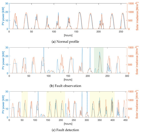
Figure 5.
Profiles of PV power and solar irradiance for (a) normal, (b) fault injected, and (c) fault detected days.The green-shaded profile in (b) denotes a missing fault and the yellow-shaded profiles in (c) correspond to false alarms occurring at site 12.
5.3. Analysis of Fault Imputation Result
The imputation accuracy computed with the NRMSE metric is presented in Table 9. As generally expected, most of the sites in the PV fleet show improved imputation performance when using each other self-labeled PV data, corresponding to Cases 4 or 5 as their overall NRMSEs are the lowest at 0.2359 and 0.2367, respectively. Comparing to Case 2 (only SWS data utilized), where overall imputation accuracy is 0.2925, the improvement is shown to be 19.35% and 19.08%, respectively. Likewise compared to Case 3 (PV without label) where NRMSE is 0.2888, Cases 4 and 5 have been improved by 18.32% and 18.04%, respectively. In addition, as depicted in Figure 6, Cases 4 and 5 are shown to have slightly tighter deviations in comparison with the other cases, which means more stable. In the following we present the details for each imputation case.
Table 9.
Imputation normalized root mean square error (NRMSE).
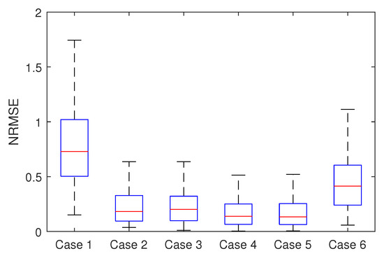
Figure 6.
Boxplot of imputation NRMSE for each imputation case.
Case 1 supposed that only historical PV data from a certain site is applicable, which means that information is restricted when considering weather variations. Therefore, an AR model was constructed in this case that focused only on the periodicity of the operation time without reflecting climatic properties. The imputation result showed insufficient performance compared to the other case studies for all sites in the fleet. Case 2 was a general case that applied the nearest meteorological data. The weather stations were lacking in the fleet, which resulted in representative station data being used after all. We concluded that when the PV site was close to the weather station, Case 2 showed better performance than when using surrounding PV data. For example, the imputation results from sites 3 and 4 that belonged to G2 were the best in this case. Case 3 used additional data obtained from neighboring PV systems beyond the labels of the system conditions. Because abnormal patterns were not removed in the previous stage, they were fed into the imputation phase as provided. This case was feasible only when the assumption that faults do not occur was satisfied. Case 4 was used to examine the effectiveness of a neighbor PV generation profile with labeled status. Because normal profiles were selected as candidates of explanatory data for the regression model, they showed reliable imputation results. In particular, PV sites from G4 showed improved results to those used in Case 2. This was because, even though the groups were slightly away from the weather station, they were crowded collectively, which provided more relevant information on the PV power output than distant weather data. As mentioned earlier, Case 5 merged Cases 2 and 4. It is observed that only sites in close distance to SWS have effects on combining SWS data to neighbor PVs. Otherwise, it did not appear to have a significant effect in faraway PVs despite of belonging to PV fleet. This demonstrates that even neighboring PVs in the same fleet have subtle differences in solar irradiance. The kNN in Case 6 shows low performance in PV fleet fault imputation. Since it depends on similar historical patterns of solar irradiance, it may not reflect random fluctuation especially in overcasting day which results in low imputation accuracy.
6. Conclusions
This paper presents a framework for PV fault detection and imputation method on PV fleets without the manual annotation of the state of the PV systems. We supplement the meteorological data measured at LWS, which had a relatively low value for the cross-correlation with PV generation, using the neighboring PV fleet data. Several features were derived to be used as input for K-means clustering to label normal or abnormal patterns. PV fleet on the campus and solar irradiance data measured at one of the PV sites in the fleet were utilized to extract the features for fault pattern detection. We arbitrarily injected a fault pattern based on actual observations, and the detection accuracy was evaluated using a confusion matrix. The detection error rate was compared for three cases: Using SolarClique (a conventional prediction-based detection method), a clustering-based method without PV fleet data, and a clustering-based method with PV fleet data which is the proposed method. The error rates for these three cases were 0.0753, 0.0223, and 0.0126, which means that the proposed clustering-based detection using neighboring PV fleet data can effectively detect the faults.
Data imputation was conducted for the distinguished abnormal patterns. Five cases of regression-based imputation and kNN were evaluated by NRMSE. In general, Cases 4 and 5, which utilized neighboring self-labeled PV data, showed better imputation performance than imputation without nearby sites or without labeled PV data by reducing NRMSE over 19% and 18%, respectively. In addition, according to earlier grouping information based on cross-correlation analysis, G3, which were close SWS, generally showed better performance when only solar irradiance data were used. However, the imputation result for G3 sites and neighboring PV profiles provided more relevant information than weather data obtained at SWS that was relatively far away. In summary, neighboring PV data are effective in improving fault detection and imputation accuracy in a dense PV fleet.
Author Contributions
All authors contributed to this work by collaboration. S.P. (Sunme Park) developed the idea and methodologies and is the first author in this manuscript. S.P. (Soyeong Park) reviewed previous literature and conducted data analysis for implementation, M.K. conducted detection performance comparisons and E.H. led and supervised the research and is the corresponding author. All authors have read and agreed to the published version of the manuscript.
Funding
This research was funded by the ETRI R&D program (19ZK1140) and the government of Korea and by the Korea Institute of Energy Technology Evaluation and Planning (KETEP).
Acknowledgments
This work was supported by the ETRI R&D program (19ZK1140), funded by the government of Korea and by the Korea Institute of Energy Technology Evaluation and Planning (KETEP) and the Ministry of Trade, Industry and Energy (MOTIE) of the Republic of Korea (No. 20171210200810).
Conflicts of Interest
The authors declare no conflict of interest.
Abbreviations
The following abbreviations are used in this manuscript:
| Feature associated with candidate PV and solar irradiance | |
| Feature associated with candidate PV and neighboring PVs | |
| N | Total number of PVs in PV fleet |
| n | ID number of candidate PV |
| k | ID number of neighboring PVs i.e., |
| t | Hourly time index |
| T | Set of PV operation time indexes |
| Duration of T | |
| Daily profile of PV | |
| Daily profile of solar irradiance |
References
- Mellit, A.; Tina, G.M.; Kalogirou, S.A. Fault detection and diagnosis methods for photovoltaic systems: A review. Renew. Sustain. Energy Rev. 2018, 91, 1–17. [Google Scholar] [CrossRef]
- Pvps, I. Strategic PV Analysis and Outreach. 2019. Available online: http://www.iea-pvps.org/fileadmin/dam/public/report/statistics/IEA-PVPS_T1_35_Snapshot2019-Report.pdf (accessed on 27 November 2019).
- Murdock, H.E.; Gibb, D.; André, T.; Appavou, F.; Brown, A.; Epp, B.; Kondev, B.; McCrone, A.; Musolino, E.; Ranalder, L.; et al. Renewables 2019 Global Status Report; UNEP: Nairobi, Kenya, 2019. [Google Scholar]
- Firth, S.K.; Lomas, K.J.; Rees, S.J. A simple model of PV system performance and its use in fault detection. Solar Energy 2010, 84, 624–635. [Google Scholar] [CrossRef]
- Daliento, S.; Chouder, A.; Guerriero, P.; Pavan, A.M.; Mellit, A.; Moeini, R.; Tricoli, P. Monitoring, diagnosis, and power forecasting for photovoltaic fields: A review. Int. J. Photoenergy 2017, 2017. [Google Scholar] [CrossRef]
- Yoon, S.; Hwang, E. Load Guided Signal-Based Two-Stage Charging Coordination of Plug-In Electric Vehicles for Smart Buildings. IEEE Access 2019, 7, 144548–144560. [Google Scholar] [CrossRef]
- Park, K.; Yoon, S.; Hwang, E. Hybrid load forecasting for mixed-use complex based on the characteristic load decomposition by pilot signals. IEEE Access 2019, 7, 12297–12306. [Google Scholar] [CrossRef]
- McCandless, T.C.; Haupt, S.E.; Young, G.S. The effects of imputing missing data on ensemble temperature forecasts. J. Comput. 2011, 6, 162–171. [Google Scholar] [CrossRef][Green Version]
- McCandless, T.; Haupt, S.; Young, G.S. A model tree approach to forecasting solar irradiance variability. Solar Energy 2015, 120, 514–524. [Google Scholar] [CrossRef]
- Hoff, T.E.; Perez, R. Quantifying PV power output variability. Solar Energy 2010, 84, 1782–1793. [Google Scholar] [CrossRef]
- Perez, R.; Kivalov, S.; Schlemmer, J.; Hemker, K., Jr.; Hoff, T.E. Short-term irradiance variability: Preliminary estimation of station pair correlation as a function of distance. Solar Energy 2012, 86, 2170–2176. [Google Scholar] [CrossRef]
- Hoff, T.E.; Perez, R. PV power output variability: Correlation coefficients. In Research Report of Clean Power Research; Clean Power Research: Napa, CA, USA, 2010. [Google Scholar]
- Widén, J. A model of spatially integrated solar irradiance variability based on logarithmic station-pair correlations. Solar Energy 2015, 122, 1409–1424. [Google Scholar] [CrossRef]
- Alsafasfeh, M.; Abdel-Qader, I.; Bazuin, B.; Alsafasfeh, Q.; Su, W. Unsupervised Fault Detection and Analysis for Large Photovoltaic Systems Using Drones and Machine Vision. Energies 2018, 11, 2252. [Google Scholar] [CrossRef]
- Chine, W.; Mellit, A.; Lughi, V.; Malek, A.; Sulligoi, G.; Pavan, A.M. A novel fault diagnosis technique for photovoltaic systems based on artificial neural networks. Renew. Energy 2016, 90, 501–512. [Google Scholar] [CrossRef]
- Garoudja, E.; Harrou, F.; Sun, Y.; Kara, K.; Chouder, A.; Silvestre, S. Statistical fault detection in photovoltaic systems. Solar Energy 2017, 150, 485–499. [Google Scholar] [CrossRef]
- Espinoza Trejo, D.; Bárcenas, E.; Hernández Díez, J.; Bossio, G.; Espinosa Pérez, G. Open-and short-circuit fault identification for a boost dc/dc converter in PV MPPT systems. Energies 2018, 11, 616. [Google Scholar] [CrossRef]
- Islam, H.; Mekhilef, S.; Shah, N.B.M.; Soon, T.K.; Seyedmahmousian, M.; Horan, B.; Stojcevski, A. Performance evaluation of maximum power point tracking approaches and photovoltaic systems. Energies 2018, 11, 365. [Google Scholar] [CrossRef]
- Chen, Z.; Han, F.; Wu, L.; Yu, J.; Cheng, S.; Lin, P.; Chen, H. Random forest based intelligent fault diagnosis for PV arrays using array voltage and string currents. Energy Convers. Manag. 2018, 178, 250–264. [Google Scholar] [CrossRef]
- Madeti, S.R.; Singh, S. Modeling of PV system based on experimental data for fault detection using kNN method. Solar Energy 2018, 173, 139–151. [Google Scholar] [CrossRef]
- Harrou, F.; Sun, Y.; Taghezouit, B.; Saidi, A.; Hamlati, M.E. Reliable fault detection and diagnosis of photovoltaic systems based on statistical monitoring approaches. Renew. Energy 2018, 116, 22–37. [Google Scholar] [CrossRef]
- Platon, R.; Martel, J.; Woodruff, N.; Chau, T.Y. Online fault detection in PV systems. IEEE Trans. Sustain. Energy 2015, 6, 1200–1207. [Google Scholar] [CrossRef]
- Zhao, Y.; Lehman, B.; Ball, R.; Mosesian, J.; de Palma, J.F. Outlier detection rules for fault detection in solar photovoltaic arrays. In Proceedings of the 2013 Twenty-Eighth Annual IEEE Applied Power Electronics Conference and Exposition (APEC), Long Beach, CA, USA, 17–21 March 2013; pp. 2913–2920. [Google Scholar]
- Alam, M.; Muttaqi, K.M.; Sutanto, D. A SAX-based advanced computational tool for assessment of clustered rooftop solar PV impacts on LV and MV networks in smart grid. IEEE Trans. Smart Grid 2013, 4, 577–585. [Google Scholar] [CrossRef]
- Mekki, H.; Mellit, A.; Salhi, H. Artificial neural network-based modelling and fault detection of partial shaded photovoltaic modules. Simul. Model. Pract. Theory 2016, 67, 1–13. [Google Scholar] [CrossRef]
- Pérez-Ortiz, M.; Jiménez-Fernández, S.; Gutiérrez, P.A.; Alexandre, E.; Hervás-Martínez, C.; Salcedo-Sanz, S. A review of classification problems and algorithms in renewable energy applications. Energies 2016, 9, 607. [Google Scholar] [CrossRef]
- Jones, C.B.; Stein, J.S.; Gonzalez, S.; King, B.H. Photovoltaic system fault detection and diagnostics using Laterally Primed Adaptive Resonance Theory neural network. In Proceedings of the 2015 IEEE 42nd Photovoltaic Specialist Conference (PVSC), New Orleans, LA, USA, 14–19 June 2015; pp. 1–6. [Google Scholar]
- Jazayeri, K.; Jazayeri, M.; Uysal, S. Artificial neural network-based all-sky power estimation and fault detection in photovoltaic modules. J. Photonics Energy 2017, 7, 025501. [Google Scholar] [CrossRef]
- Dhimish, M.; Holmes, V.; Mehrdadi, B.; Dales, M. Comparing Mamdani Sugeno fuzzy logic and RBF ANN network for PV fault detection. Renew. Energy 2018, 117, 257–274. [Google Scholar] [CrossRef]
- Chouay, Y.; Ouassaid, M. An intelligent method for fault diagnosis in photovoltaic systems. In Proceedings of the 2017 International Conference on Electrical and Information Technologies (ICEIT), Rabat, Morocco, 15–18 November 2017; pp. 1–5. [Google Scholar]
- Jiang, L.L.; Maskell, D.L. Automatic fault detection and diagnosis for photovoltaic systems using combined artificial neural network and analytical based methods. In Proceedings of the 2015 International Joint Conference on Neural Networks (IJCNN), Killarney, Ireland, 12–17 July 2015; pp. 1–8. [Google Scholar]
- Garoudja, E.; Chouder, A.; Kara, K.; Silvestre, S. An enhanced machine learning based approach for failures detection and diagnosis of PV systems. Energy Convers. Manag. 2017, 151, 496–513. [Google Scholar] [CrossRef]
- Zhu, H.; Lu, L.; Yao, J.; Dai, S.; Hu, Y. Fault diagnosis approach for photovoltaic arrays based on unsupervised sample clustering and probabilistic neural network model. Solar Energy 2018, 176, 395–405. [Google Scholar] [CrossRef]
- Akram, M.N.; Lotfifard, S. Modeling and health monitoring of DC side of photovoltaic array. IEEE Trans. Sustain. Energy 2015, 6, 1245–1253. [Google Scholar] [CrossRef]
- Wang, Z.; Balog, R.S. Arc fault and flash detection in photovoltaic systems using wavelet transform and support vector machines. In Proceedings of the 2016 IEEE 43rd Photovoltaic Specialists Conference (PVSC), Portland, OR, USA, 5–10 June 2016; pp. 3275–3280. [Google Scholar]
- Yi, Z.; Etemadi, A.H. A novel detection algorithm for line-to-line faults in photovoltaic (PV) arrays based on support vector machine (SVM). In Proceedings of the 2016 IEEE Power and Energy Society General Meeting (PESGM), Boston, MA, USA, 17–21 July 2016; pp. 1–4. [Google Scholar]
- Jufri, F.H.; Oh, S.; Jung, J. Development of Photovoltaic abnormal condition detection system using combined regression and Support Vector Machine. Energy 2019, 176, 457–467. [Google Scholar] [CrossRef]
- Zhao, Y.; Yang, L.; Lehman, B.; de Palma, J.F.; Mosesian, J.; Lyons, R. Decision tree-based fault detection and classification in solar photovoltaic arrays. In Proceedings of the 2012 Twenty-Seventh Annual IEEE Applied Power Electronics Conference and Exposition (APEC), Orlando, FL, USA, 5–9 February 2012; pp. 93–99. [Google Scholar]
- Belaout, A.; Krim, F.; Mellit, A.; Talbi, B.; Arabi, A. Multiclass adaptive neuro-fuzzy classifier and feature selection techniques for photovoltaic array fault detection and classification. Renew. Energy 2018, 127, 548–558. [Google Scholar] [CrossRef]
- Chen, Z.; Wu, L.; Cheng, S.; Lin, P.; Wu, Y.; Lin, W. Intelligent fault diagnosis of photovoltaic arrays based on optimized kernel extreme learning machine and IV characteristics. Appl. Energy 2017, 204, 912–931. [Google Scholar] [CrossRef]
- Liao, Z.; Wang, D.; Tang, L.; Ren, J.; Liu, Z. A heuristic diagnostic method for a PV system: Triple-layered particle swarm optimization–back-propagation neural network. Energies 2017, 10, 226. [Google Scholar] [CrossRef]
- Zhao, Y.; Ball, R.; Mosesian, J.; de Palma, J.F.; Lehman, B. Graph-based semi-supervised learning for fault detection and classification in solar photovoltaic arrays. IEEE Trans. Power Electron. 2014, 30, 2848–2858. [Google Scholar] [CrossRef]
- Zhao, Q.; Shao, S.; Lu, L.; Liu, X.; Zhu, H. A new PV array fault diagnosis method using fuzzy C-mean clustering and fuzzy membership algorithm. Energies 2018, 11, 238. [Google Scholar] [CrossRef]
- Lin, P.; Lin, Y.; Chen, Z.; Wu, L.; Chen, L.; Cheng, S. A density peak-based clustering approach for fault diagnosis of photovoltaic arrays. Int. J. Photoenergy 2017, 2017. [Google Scholar] [CrossRef]
- Ding, H.; Ding, K.; Zhang, J.; Wang, Y.; Gao, L.; Li, Y.; Chen, F.; Shao, Z.; Lai, W. Local outlier factor-based fault detection and evaluation of photovoltaic system. Solar Energy 2018, 164, 139–148. [Google Scholar] [CrossRef]
- Harrou, F.; Dairi, A.; Taghezouit, B.; Sun, Y. An unsupervised monitoring procedure for detecting anomalies in photovoltaic systems using a one-class Support Vector Machine. Solar Energy 2019, 179, 48–58. [Google Scholar] [CrossRef]
- Korea Weather Information (Korean). Available online: https://data.kma.go.kr/cmmn/main.do (accessed on 27 November 2019).
- Wang, F.; Zhen, Z.; Mi, Z.; Sun, H.; Su, S.; Yang, G. Solar irradiance feature extraction and support vector machines based weather status pattern recognition model for short-term photovoltaic power forecasting. Energy Build. 2015, 86, 427–438. [Google Scholar] [CrossRef]
- Shams, M.B.; Haji, S.; Salman, A.; Abdali, H.; Alsaffar, A. Time series analysis of Bahrain’s first hybrid renewable energy system. Energy 2016, 103, 1–15. [Google Scholar] [CrossRef]
- Iyengar, S.; Lee, S.; Sheldon, D.; Shenoy, P. Solarclique: Detecting anomalies in residential solar arrays. In Proceedings of the 1st ACM SIGCAS Conference on Computing and Sustainable Societies, San Jose, CA, USA, 20–22 June 2018; p. 38. [Google Scholar]


© 2020 by the authors. Licensee MDPI, Basel, Switzerland. This article is an open access article distributed under the terms and conditions of the Creative Commons Attribution (CC BY) license (http://creativecommons.org/licenses/by/4.0/).