Abstract
The implicit model of photovoltaic (PV) arrays in series-parallel (SP) configuration does not require the LambertW function, since it uses the single-diode model, to represent each submodule, and the implicit current-voltage relationship to construct systems of nonlinear equations that describe the electrical behavior of a PV generator. However, the implicit model does not analyze different solution methods to reduce computation time. This paper formulates the solution of the implicit model of SP arrays as an optimization problem with restrictions for all the variables, i.e., submodules voltages, blocking diode voltage, and strings currents. Such an optimization problem is solved by using two deterministic (Trust-Region Dogleg and Levenberg Marquard) and two metaheuristics (Weighted Differential Evolution and Symbiotic Organism Search) optimization algorithms to reproduce the current–voltage (I–V) curves of small, medium, and large generators operating under homogeneous and non-homogeneous conditions. The performance of all optimization algorithms is evaluated with simulations and experiments. Simulation results indicate that both deterministic optimization algorithms correctly reproduce I–V curves in all the cases; nevertheless, the two metaheuristic optimization methods only reproduce the I–V curves for small generators, but not for medium and large generators. Finally, experimental results confirm the simulation results for small arrays and validate the reference model used in the simulations.
1. Introduction
The continuous effects of climate change and environmental contamination have motivated a growing interest in the use of renewable energies to replace conventional energy sources based on fossil fuels. Within renewable energies, photovoltaic (PV) energy offers interesting advantages: long life cycle, lack of mobile parts, low maintenance costs, modularity, among others [1]; that is why the installed PV capacity has been growing in the last years [2]. In a PV system, one of the most important elements is the generator; therefore, it is important to have models of this element to reproduce its electrical behavior when they operate under homogeneous and non-homogeneous conditions [3]. These models are used in different applications like the sizing of PV generators, the power, and energy production estimation, the analysis, and evaluation of maximum power point tracking techniques, model-based diagnosis, and other applications [4]. A PV generator can be connected in different configurations, nonetheless, series-parallel (SP) is one of the most used configurations. In an SP generator, two or more modules are connected in series to form a string and two or more strings are connected in parallel to form the generator. As a consequence, all the strings have the same voltage and can be analyzed independently [5]. It is worth noting that each module is formed by one or more submodules connected in series and each submodule has a bypass diode connected in antiparallel. When the irradiance and temperature of all the submodules in the generator are the same, it can be said that the generator operates under homogeneous conditions [6]. In these conditions, the whole generator can be represented by the single-diode model (SDM) scaled in voltage, according to the number of modules in the string, and scaled in current, according to the number of strings in parallel [7]. In this case, the current vs. voltage (I–V) curve has a single knee and the power vs. voltage (P-V) curve has a single maximum power point (MPP), which can be easily tracked. In real applications, the PV generator is commonly shaded, or partially shaded, by surrounding objects, passing clouds, or other objects. Hence, the operating conditions (i.e., irradiance and temperature) of the shaded submodules are different than the operating conditions of the rest of the submodules [8]. In this case, it is said that the generator operates in nonhomogeneous conditions and the generator’s I–V curve may present multiple knees, which is translated into multiple MPPs in the P-V curve [9]. To model a PV generator operating in nonhomogeneous conditions, it is necessary to consider that each submodule in a module is represented by the SDM. In this way, it is possible to include the effects of the nonhomogeneous conditions in the electrical behavior of the generator [10]. Therefore, the generator can be analyzed as an equivalent circuit that is obtained by connecting strings in parallel, where each string is formed by a set of submodules connected in series [11,12].
In the literature, most of the models use the SDM to represent each submodule and they use the LambertW function [13] to obtain an explicit equation of the submodule’s current as a function of its voltage [7,14,15,16]. Then, each string formed by N submodules and a blocking diode is modeled independently by a system of N + 1 nonlinear equations, where the unknowns are the voltages of the blocking diode and the N submodules [7,14,15,16]. Solving the system of nonlinear equations of each string, it is simple to calculate the string current and finally the generator’s current. However, the evaluation of the LambertW function implies a high computational cost for the solution to the system of nonlinear equations associated with each string. For example, in [7] the modeling of a PV array based on the use of the Lambert W-function to obtain an explicit relationship between the voltage and current of any PV module is presented. In addition, the non-linear equations that describe the PV array are solved by means of explicit symbolic calculation of the inverse of the Jacobian matrix. A similar solution was published in [14], where a new formulation of the one-diode model of the PV module is solved using the LambertW function with the terminal voltage expressed as an explicit function of the current, this approximation resulting in a reduction of simulation calculation time. Another solution was presented in [16], where a model of the PV field is presented by means of a set non-linear equations characterized by a sparse Jacobian matrix, which requires a moderate computational burden, both in terms of memory use and processor speed. Optimization methods for estimating the PV module parameters are presented as a suitable option to overcome the drawbacks of deterministic and iterative methods. In addition, optimization methods are not only used in PV area for estimating parameters, since the reconfiguration of PV modules to mitigate the effect of partial shading conditions in PV arrays is currently one of the most studied topics [17]. The model proposed in [18] uses the implicit equation that describes the current-voltage relationship in the SDM. From such an equation, is it possible to construct a system of N + 2 implicit equations to model each string, where the unknowns are the string current and the N + 1 voltages of the N submodules and the blocking diode. Then, solving each string it is possible to calculate the generator’s current as in the other models. In [18] the system of N + 2 implicit equations is solved by using the Trust-Region Dogleg (TRD) algorithm, which is a deterministic optimization method. However, the authors in [18] do not formulate the solution of the system of N + 2 implicit equations as an optimization problem with restrictions; moreover, the authors do not provide any justification for the selection of TRD for solving the optimization problem nor evaluate other deterministic and metaheuristic optimization algorithms. Finally, those works [7,14,15,16,18] are focused on the model, i.e., the system of nonlinear equations, and not in the optimization algorithms used to solve such models. Therefore, from those papers it is not clear which type of optimization methods should be used to reduce the calculation time.
This paper formulates the solution of the system of N + 2 implicit equations, associated with each string, as an optimization problem with restriction for the N + 2 unknowns, i.e., string current and the voltages of the N modules and the blocking diode. Moreover, the paper evaluates four optimization algorithms, two deterministic and two metaheuristics, to solve the problem and generate the I–V and P-V curves of generators with different sizes. The two deterministic algorithms are TRD and Levenberg-Marquardt (LMA), which are widely used to solve optimization problems in different areas; while the two metaheuristic optimization algorithms are Weighted Differential Evolution (WDE) and Symbiotic Organism Search (SOS), which have been recently used for PV applications. The evaluation of the optimization algorithms is performed with simulations of small, medium, and large generators in homogeneous and non-homogeneous conditions. Finally, experimental results are used to evaluate the different optimization algorithms for a small PV generator. In light of the previous analysis, the main advantages of the proposed procedure are listed as follows:
- A solution of the system of N + 2 implicit equation as an optimization problem with restrictions, which can be used to explore other optimization methods to reduce the model’s solution time.
- Performance comparison of metaheuristic and deterministic optimization algorithms for solving the problem provides guidelines to continue exploring other optimization methods to reduce the computation time.
- A novel application of the algorithms of weighted differential evolution and search for symbiotic organisms to solve the implicit model of series-parallel photovoltaic arrays is presented.
The rest of the paper is organized as follows: Section 2 describes the implicit model used in this paper, Section 3 introduces the optimization problem and the operating principle of the optimization algorithms, Section 4 and Section 5 show the simulation and experimental results, respectively, and Section 6 closes the paper with the conclusions.
2. Implicit Model of a Series-Parallel Generator
This section shows a brief description of the implicit model of SP generators proposed in [18], which includes the SDM used to represent each submodule, the system of N + 2 implicit equation of each string, and the calculation of the array current.
2.1. Submodule Model
The SDM (see Figure 1) has been widely used in the literature to represent the electrical behavior of PV submodules [10,19,20], which can be defined as a set of cells connected in series. Such a model is able to represent mono-crystalline and poly-crystalline PV cells technologies [20]; in this paper PV modules formed by poly-crystalline cells have been used in simulation and experimental validations. In the SDM, represents the current generated by the photovoltaic effect, the diode D models the nonlinearities of the PN junction, and the resistors and represent the leakage currents and ohmic losses, respectively. The bypass diode (BD) is an additional connected in antiparallel to the submodule (see Figure 1) to limit the power dissipated in the cells in mismatching conditions. The calculation of the PV module parameters has been widely reported in literature, not only for the SDM model [21] but also for the two-diode [22] and three-diode model [23]. Nevertheless, the estimating parameter techniques have been more widely studied for the SDM. Such an issue has been addressed by means of different approaches which can be grouped into: analytical, deterministic and metaheuristic [24,25]. The first two groups present drawbacks concerning accuracy and convergence. Therefore, metaheuristic algorithms have been introduced as an attractive alternative for estimating the PV cells and modules parameters [25]. Such approaches may include particle swarm optimization [26], genetic algorithms [27], differential evolution [28], cuckoo search [29], among others.
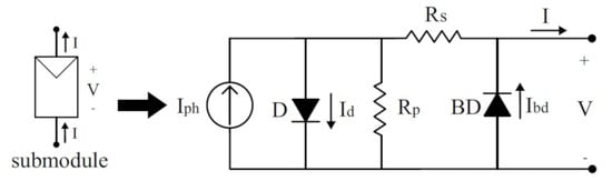
Figure 1.
Submodule model including the bypass diode.
From the circuit shown in Figure 1, it is possible to write an implicit equation that describes the relationship between the submodule’s output voltage (V) and current (I), as shown in (1), where and are the inverse saturation current, and ideality factor of D, respectively, is the diode thermal voltage and is the current through BD. The thermal voltage is defined as , where k is the Boltzmann constant, q is the electron charge and T is the cell’s temperature in K. Moreover, is defined in (2), where and are the inverse saturation current and ideality factor of BD. It is worth noting that is the same for diodes D and BD since it can be assumed that the cell’s temperature and the bypass diode temperature are the same if there isn’t a fast change in the irradiance [30].
Although the SDM parameters (i.e., and ) may vary with the irradiance and temperature [31,32,33], is directly proportional to the irradiance; therefore, it can be used as an indication of the incident irradiance on the submodule.
2.2. Generator’s Model
In general, an SP generator is formed by M parallel-connected strings (see Figure 2), where each string is formed by a set of PV modules () and a blocking diode connected in series. In turn, each module is formed by one or more submodules connected in series (); then, each string is formed by N submodules, where . The generator is connected to a power converter, which sets the generator voltage () to perform the MPP tracking; therefore, is known for the model and the objective is to find: the generator current (), the current of each string, the voltage of each submodule, and the voltage of each blocking diode.
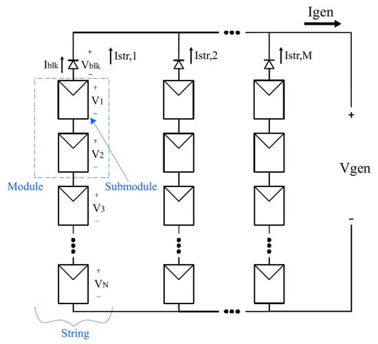
Figure 2.
Series–parallel photovoltaic generator with M strings, of N submodules each, connected in parallel, where each string includes a blocking diode and each module has two submodules.
Considering the is common for all the strings, each string can be analyzed and solved independently. Then, a string formed by N submodules and a blocking diode connected in series can be represented by a system of N + 2 nonlinear and implicit equations, as shown in (3) [18]; where is a vector formed by the voltages of the N submodules and the blocking diode () and is the string current.
The first N equations of (3), correspond the voltage-current relationship in each submodule given in (1), while equation N + 1 describes the model of the blocking diode and it is described in (4), where , and are the inverse saturation current and the ideality factor of the blocking diode, respectively, and is the diode thermal voltage defined in Section 2.1, since the blocking diode temperature is assumed the same of the submodules. Finally, equation N + 2 in (3) is obtained from the Kirchhoff voltage law in the loop formed with the string and .
3. Optimization Problem Formulation and Solution Methods
This Section defines the solution of (3) as an optimization problem with its restrictions and presents a brief explanation of the optimization algorithms used in the paper to solve the optimization problem.
3.1. Optimization Problem and Restrictions
Let be the set of real numbers and a non-empty subset of , i.e., ; then, the system of nonlinear equations given in (3) can be expressed as shown in (6), where and . The solution of (6) is given by all vectors , such that .
Now, let’s consider the function a function defined as shown in (7).
Note that is a well-defined function that guarantees the existence of a minimum, since for all is a totally ordered set where exists the infimum of and this infimum is non-negative, i.e., . Therefore, the minimum of over exists and it is a non-negative minimum.
Theorem 1.
Proof.
If is a solution of the system of equations given in (3), then , therefore, . Moreover, considering that for all , then is the minimum point of . Now, if minimizes but it is not a solution of (3), then must be positive, since for all . Taking into account that (3) has a solution in , then there is a solution such that and . Hence, , which contradicts that is a minimum point for . ▢
The last paragraph proves that the minimum point of the objective function given in (7) is the set of values that solve the system of equations shown in (3). Such a solution contains the unknown voltages in the string () and the string current (). However, to minimize (7) using numerical methods, it is necessary to establish the limits of and each unknown in as shown in Table 1.

Table 1.
Upper and lower limits of the electrical variables in a string.
The lower limit of the string current is 0 A; while the upper limit is , which corresponds to the submodule short-circuit current in Standard Test Conditions (STC), i.e., irradiance of 1 kW/m2 and the submodule temperature is 25 °C (i.e., = 298.15 K). Moreover, the upper limit of the submodules voltages () is open-circuit voltage in STC (), which corresponds to the submodule voltage when A. The lower limit of is the negative value of the maximum bypass diode voltage (), defined in (8), which corresponds to the bypass diode voltage when . This current corresponds to the worst-case scenario where the submodule is completely shaded, and the string current is maximum. Finally, the upper limit of the blocking diode voltage is 0 V, which corresponds to A; while the lower limit corresponds to the negative value of the maximum blocking diode voltage () defined in (9).
3.2. Optimization Methods
This section presents a brief description of the optimization algorithms used to minimize the objective function introduced in (7) and to find the solution to the system of nonlinear equations associated with the string (3).
3.2.1. Trust-Region Dogleg (TRD)
This is a deterministic algorithm with a single search agent. It starts from an initial point , that belongs to the domain of , and searches the point that minimizes the function f through the iterative process indicated in (10), where is the actual position of the search agent and is the step of the k-th iteration.
To determine the magnitude and direction of the vector that approaches to is posed as an optimization problem, as shown in (11), where is an approximate function of formed by the two first terms of the Taylor series in a region that contains .
If is a good approximation of the objective function in a region , then this region is denominated thrust-interval and it is defined as , where is the radius of the thrust-region in the k-th iteration. Once the vector is found, i.e., the solution of (11), it is necessary to verify the fulfillment of the condition expressed in (12).
If condition (12) is fulfilled, the actual position is updated as ; then, the next step is to calculate a new model and a new trust-region from the updated point . Otherwise, if condition (12) is not fulfilled, the algorithm keeps the actual position, i.e., , and the trust-region is reduced by reducing its radius (). The details of this algorithm can be found in [34] along with different variants of this method.
3.2.2. Levenberg-Marquardt (LMA)
This is a deterministic optimization algorithm that requires the calculation of the jacobian matrix (J) and it is especially effective for solving nonlinear problems, where methods that used linear models, like Gauss–Newton, are not effective for the entire solution region [35]. The essence of this method is to select the search direction of the next step between the one given by the Gauss–Newton method and a direction close to the one provided by the gradient descent method. That direction search is selected by a criterion denominated .
Let’s consider an optimization problem that has the structure of a trust-interval, as shown in (13) and (14) [35].
This is a least-squares problem, which is linear with restrictions because is a linearized model valid in the trust-region defined by . The solution to the problem described in (13) and (14) is obtained by solving (15), where , and the position of the next iteration is given by (16) [35].
When , then and (16) is solved by ; in this case, the best search direction is the same as the Gauss–Newton method. Otherwise, and the solution of (16) fulfills ; with this condition, it is possible to find the solution of (16) and the value of . When , the search direction is close to the one of the gradient descent method and (15) approaches to (17). Further details of the Levenberg–Marquardt algorithm are provided in [35].
3.2.3. Weighted Differential Evolution (WDE)
This metaheuristic optimization method uses the evolution concept to solve numerical optimization problems and it is characterized by calculating the search direction and the search steps in an evolutionary way [36]. The general process of the WDE algorithm is introduced in Figure 3, where the first step is to generate two populations denominated initial population (P) and subpopulation (SubP), both randomly created with a normal distribution. Then, SubP is mutated to create TempP and vector F and binary map M are generated, by using random variables. Population SubP, F and M are used in a mutation and crossover proves to generate the new population (T), which requires verification that all the individuals fulfill the problem restrictions (boundaries control). The individuals that do not fulfill the restrictions are adjusted to be within the problem borders. Now, the objective function is evaluated for all the individuals of T and SubP and the best individuals in both populations are identified ( and ). If is a better solution than , then is updated ( = ), and population P is updated from SubP; otherwise, TempP, F and M are calculated to generate a new T. Finally, the best individual of P is evaluated to verify if it fulfills the stop criteria; else, a new algorithm iteration starts.
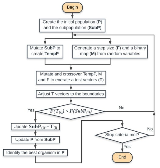
Figure 3.
Flow chart of the weighted differential evolution algorithm.
3.2.4. Symbiotic Organism Search (SOS)
This is a metaheuristic optimization algorithm inspired by the different interactions between the living beings of different species that share an ecosystem, named symbiotic relationships. The first phase of the algorithm is to create an initial population of particles that represents an ecosystem, and each particle represents an organism. Then, it is necessary to define some parameters, like the solution boundaries and the stop criteria, before starting the iterative process, which is based on three types of relationships: mutualism, commensalism, and parasitism. In the mutualism phase, two organisms participate, and , where is the i-th organism into the ecosystem and is a randomly chosen organism within the ecosystem. In this phase, both organisms could be benefited from each other through the creation of a new vector () described in (18)
Then, the algorithm calculates two new candidates to replace and by using (19) and (20), which model the mutualist symbiotic relationship between two organisms. In (19) and (20) is a vector with random numbers between 0 and 1, and is the organism with the lowest value of the cost function, also known as the organism with the best adaptation in the ecosystem. Moreover, in mutualist relationships some species benefit more than the others; this phenomenon is represented by the factors and in (19) and (20), which are randomly assigned with 1 or 2. Once and are calculated, the algorithm evaluates the objective function for both organisms. If and are better solutions than and , then and replace and in the ecosystem.
In the commensalism phase, is the same organism used in the previous phase, while is an organism randomly selected from the ecosystem, but it is different than used in the mutualism stage. The commensalism relationship between and is represented by (21), where benefits from . If the objective function of the is less than the one of the objective function of , then is updated in the ecosystem.
The last symbiotic relationship is parasitism, where the organism is aleatory chosen from the ecosystem and is the same organism used in the commensalism phase, but with a random modification of one of its components. The modified is named parasite vector and if its objective function if better than , then the parasite vector replaces ; otherwise, the parasite vector is discarded, and it is said that developed immunity to the parasite. Once the three phases end for the i-th organism, the algorithm moves to the next organism to repeat the process until all the organisms in the ecosystem have been processed. At this point, one iteration if finished and the stop criteria are evaluated, if no stop condition is met, then the algorithm starts a new iteration. The detailed explanation of this algorithm is shown in [37]. Keep in mind that the evaluated algorithms (many of them) are sensitive to the assumed values for their multiple parameters. It is so sensitive that if they are not chosen with caution, they may not even converge to the expected solution even for PV arrays operating under uniform conditions. This aspect is a notable disadvantage of this metaheuristic solution strategy. Until now, there is no solid mathematical basis to predict the convergence and influence of these parameters. It is certainly possible that the results presented could have been obtained in shorter computation times, having selected other values for the algorithm parameters. However, it is worth noting that we tune the optimization algorithms in order to obtain the best results for all the algorithms. Particularly, the parameters of the metaheuristic methods selected for this work were defined randomly.
4. Simulations Results
This section introduces the simulation results for small, medium and large generators, i.e., PV generators formed by a single string with 6, 36 and 72 series-connected submodules, respectively. All the simulated generators are formed by Trina Solar TMS-PD05 de 270 W [38] modules, which are composed of three series-connected submodules. Moreover, the bypass diodes of the three submodules in this section are GF3045T [39]. It is worth noting that the generators considered in this section only have one string. This is because for generators with M strings each string is independently solved, which is equivalent to solve one string M times and then to sum the currents of all the strings to calculate the array current. The SDM parameters in STC are calculated, with the procedure proposed in [40], from the module datasheet information. Then, the parameters are adjusted for a module temperature of C (C) and an irradiance of 1 kW/m2 ( kW/m2), by following the procedure proposed in [31], obtaining the following values: A, A, , and . Afterward, the bypass diode parameters are calculated from the datasheet information as follows: A and . The irradiance condition of each submodule in the generator is represented by using the linear dependence on with the submodule irradiance. Therefore, the irradiance reduction in a submodule produced by some kind of shading is represented by a coefficient that multiplies and varies between 0 and 1. Thus the reduction of is proportional to the reduction of the submodule irradiance. The coefficients of all the string submodules are grouped in a vector () that represents the shading conditions of the string. The solutions obtained with the four optimization methods used in this paper are compared with the solution of the equivalent electrical circuit (EEC) of each generator. Those EECs for the small, medium, and large generators are implemented in Simulink of Matlab; hence, the errors calculated for the optimization algorithms are calculated concerning the EEC solution.
4.1. Small Generator
This generator is formed by two modules connected in series that correspond to six submodules. This low power generator may be used in grid-connected applications, by using a microinverter, or in stand-alone applications to charge a battery or to feed a set of lights. The simulation results of this generator operating under homogeneous (i.e., ) and partial shading (i.e., ) conditions are introduced in Figure 4 and Figure 5, respectively. Those figures show the I–V curves and the error in the current calculation for all the implemented optimization methods, which use the stop criteria shown in Table 2. Moreover, the evaluation criteria of the simulation results (see Table 3) are: the computation time, the root mean square error (RMSE), and the number of evaluations of the objective function ().
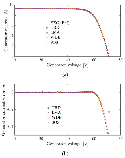
Figure 4.
Simulation results of the small generator (six submodules) under homogeneous conditions. (a) Current vs. voltage (I–V) curve. (b) Current calculation error.
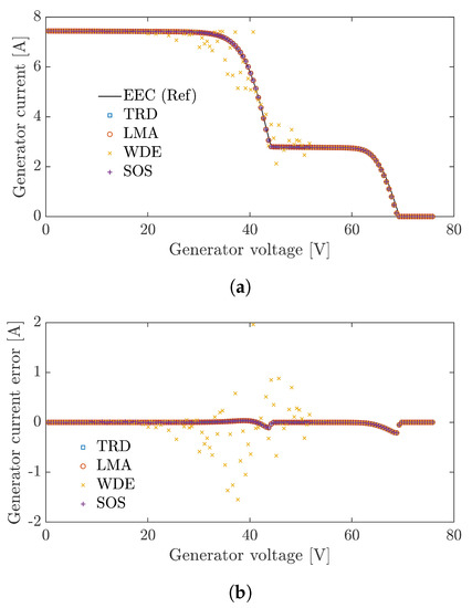
Figure 5.
Simulation results of the small generator (six submodules) under partial shading conditions. (a) Current vs. voltage (I–V) curve. (b) Current calculation error.
Table 2.
Stop criteria for the optimization methods used for the small generator.
Table 3.
Evaluation criteria for the small generator operating under homogeneous and partial shading conditions.
In Figure 4a it can be observed that all the implemented optimization methods can reproduce the I–V curve of a small string (six submodules) under homogeneous conditions. Additionally, the errors in the string current calculation are similar for the different methods, as shown in Figure 4b and Table 3. When the generator operates in partial shading conditions, three of the four algorithms (TRD, LMA, and SOS) can solve the system of implicit equations for all the voltages to reproduce the I–V with similar errors (see Figure 5 and Table 3). However, the WDE algorithm presents significant errors in the current calculation for voltages between 20 V and 55 V, as it is evidenced in Figure 5 and Table 3. Therefore, WDE is not a suitable algorithm to solve the model of a small generator in partial shading conditions. Note that under homogeneous and partial shading conditions the computation time and number of cost function evaluations () of the deterministic optimization methods (TRD and LMA) are significantly less than the computation time and of the metaheuristic algorithms (WDE and SOS), as shown in Table 3. Moreover, the RMSE values of the methods able to solve the optimization problem provide similar errors in the I–V curve reproduction.
4.2. Medium Generator
In this case, the generator is formed by one string with 12 modules (36 submodules) connected in series, which is a typical configuration for a residential application with a string inverter (e.g., ABB UNO-7.6-TL-OUTD). For this generator, the stop criteria of the optimization algorithms are modified concerning the previous subsection, as shown in Table 4, to improve the performance of the algorithms.
Table 4.
Stop criteria for the optimization methods used for the medium and large generators.
The medium generator I–V curves for homogeneous and partial shading conditions are presented in Figure 6 and Figure 7, respectively; while the computation time, RMSE and are introduced in Table 5. Moreover, the vectors that define the homogeneous () and partial shading conditions () have 36 elements and are defined as follows: all elements in are 1 and has 24 elements equal to 0.8, 6 elements equal to 0.6, and 6 elements equal to 0.2.
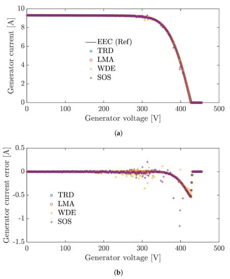
Figure 6.
Simulation results of the medium generator (36 submodules) under homogeneous conditions. (a) Current vs. voltage (I–V) curve. (b) Current calculation error.
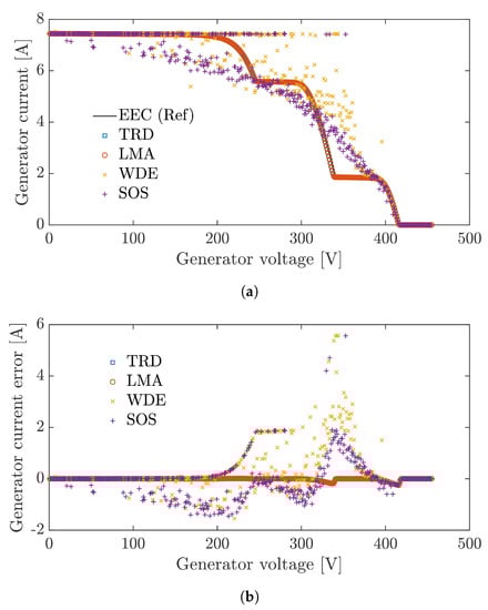
Figure 7.
Simulation results of the medium generator (36 submodules) under partial shading conditions. (a) Current vs. voltage (I–V) curve. (b) Current calculation error.
Table 5.
Evaluation criteria for the medium generator operating under homogeneous and partial shading conditions.
The results in Figure 6 and Figure 7 and Table 5 show that the deterministic methods (TRD and LMA) solve the system of equations of the string for homogeneous and partial shading conditions. Additionally, the RMSE values for the I–V curves are the same for both deterministic methods (less than 0.1 A); nevertheless, computation times of TRD are less than the computation times of LMA for both homogeneous and partial shading conditions. In general, metaheuristic methods present greater errors and computation times than the deterministic methods in the I–V curve’s calculation. For homogeneous conditions, the current errors are concentrated in medium and high generator voltages (from 250 V to 400 V), as shown in Figure 6; those errors generate RMSE values between 13% and 60% greater than the ones of the deterministic methods. Whilst for partial shading conditions, the RMSE values of the metaheuristic methods between 15.3 and 21.3 times greater than the RMSE values of the deterministic methods, and the errors occur in the entire range of the generator voltage (see Figure 7). As observed, the computation times of the metaheuristic algorithms are two orders of magnitude greater than the computation times of the deterministic methods, which is also reflected in the number of cost function evaluations (). Finally, the results in Table 5 indicate that the implemented metaheuristic optimization methods are not suitable for solving the implicit model of a medium PV generator.
4.3. Large Generator
This generator is formed by a single string with 24 modules (72 submodules) connected in series, which can be found in industrial applications or high-power generators that use inverters whit maximum input voltages of 1 kV (e.g., Sunny Tripower 20000TL). The stop criteria are the same shown in Table 4 and the vectors that define homogeneous () and partial shading () conditions have 72 elements defined as follows: all elements in () are 1 and () has 30 elements equal to 0.8, 30 elements equal to 0.6, and 12 elements equal to 0.2. The generator I–V curves and the errors in the current calculation are shown in Figure 8 and Figure 9 for homogeneous and partial shading conditions, respectively; while the computation time, RMSE and are presented in Table 6.
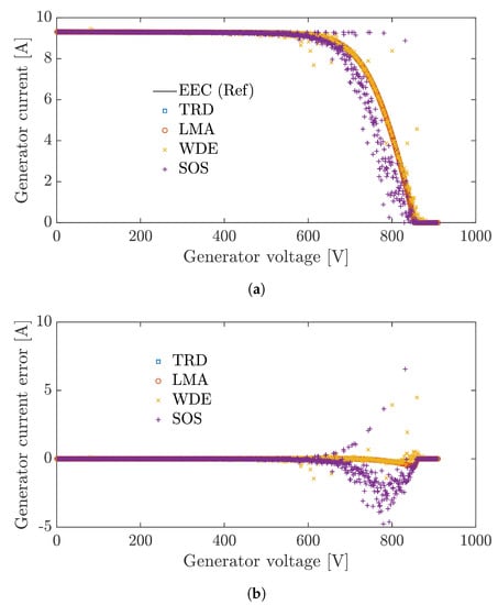
Figure 8.
Simulation results of the large generator (72 submodules) under homogeneous conditions. (a) Current vs. voltage (I–V) curve. (b) Current calculation error.
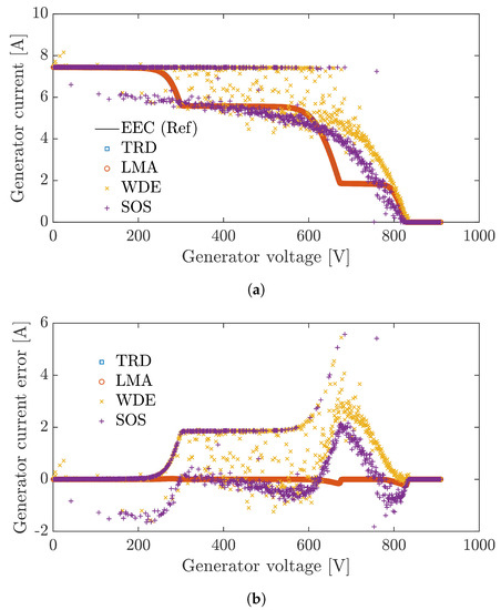
Figure 9.
Simulation results of the large generator (72 submodules) under partial shading conditions. (a) Current vs. voltage (I–V) curve. (b) Current calculation error.
Table 6.
Evaluation criteria for the large generator operating under homogeneous and partial shading conditions.
Once more, the results in Figure 8 and Figure 9 and Table 6 indicate that the deterministic optimization methods (TRD and LMA) are capable to reproduce the I–V curves for the evaluated conditions with RMSE less than 0.10 A. In homogeneous conditions, the computation time of LMA is 12.9% less than the one of TRD; while in partial shading conditions the computation time of TRD is 15.5% less than the computation time of LMA. Moreover, the values of for TRD and LMA have similar behavior to the computation time. The metaheuristic algorithms show errors and computation time greater than the deterministic algorithms in the reproduction of the I–V curves in the evaluated operating conditions. For homogeneous conditions (see Figure 8) the biggest errors are present in high voltages; as consequence, the RMSE values of the metaheuristic methods are significantly greater (between 132% and 700%) than the deterministic algorithms. In partial shading conditions (see Figure 9) the errors are in the whole voltage range, making the RMSE values of the metaheuristic methods between 24.2 and 31.9 times the RMSE values of the deterministic methods. Additionally, the computation time of the metaheuristic algorithms is two orders of magnitude greater than the one of the deterministic algorithms, which is similar to the differences in (see Table 6). After the evaluation of the four optimization algorithms for small, medium and large PV arrays, it seems that metaheuristic optimization methods do not worth their evaluations because the evaluated deterministic optimization methods outperform the evaluated metaheuristic methods. However, those results could not be obtained if the comparison is not performed; therefore, we consider that the evaluation is proposed in the paper is valid, since it is necessary to explore different optimization methods to reduce the computation time of the model. Such a reduction is important for applications like reconfiguration, energy production estimation, evaluation of MPPT techniques, among others.
5. Experimental Results
The performance of the optimization methods was validated with experimental data, which were obtained with the test bench shown in Figure 10 This test bench if formed by a PV with Matlab, a programmable electronic load BK Precision 8500, and a Trina Solar TMS-PD05 de 270 W [38] PV module. The PV module is the same one used in the simulations (formed by 3 submodules); however, the SDM parameters of the submodules ( A, nA, , and ) and the bypass diodes (A and are calculated from experimental I-V curves. The experimental validation considers two cables AWG 12 of 28.96 m each, which introduce losses that can be represented by resistance in series with the module of 313 m. Therefore, such resistance was included in the parameter of each submodule; thus, the ohmic losses introduced by the cables are lumped in the of the submodules.
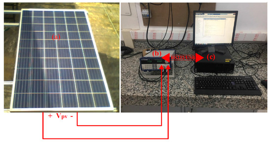
Figure 10.
Test bench used to obtain the experimental data. (a) PV module with three submodules. (b) Electronic load. (c) PC with Matlab.
The small generator used for the experimental validation was formed by one string of three submodules, which was evaluated for homogeneous (C-1) and partial shading (C-2) defined by the vectors () = [0.4 0.4 0.4] and () = [0.620 0.598 0.210], respectively. Moreover, the stop criteria used for the optimization algorithms were the same ones defined in Table 2. The experimental results for conditions C-1 and C-2 are summarized in Figure 11 and Table 7. Figure 11 introduces the I–V curves obtained with the experimental test bench, the four optimization algorithms (TRD, LMA, WDE, and SOS), and the equivalent electrical circuit (EEC) for conditions C-1 and C-2; while Table 7 shows the computation time, RMSE values, and for the different methods.
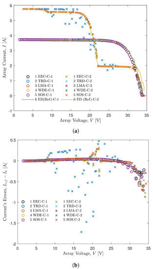
Figure 11.
Experimental results in a small generator (3 submodules) under homogeneous and partial shading conditions. (a) Current vs. voltage (I–V) curve. (b) Current calculation error.
Table 7.
Evaluation criteria for a small generator operating under homogeneous and partial shading conditions from experimental results.
In general, the experimental results agree with the simulation results obtained for small generators (Section 4.1) regarding computation time and current errors. On the one hand, in homogeneous conditions (C-1), the four optimization algorithms generate I–V curves that fit the experimental data with practically the same RMSE values. Moreover, the error in the current calculation for condition C-1 increases for high voltages (circles in Figure 11b), which agrees with the behavior shown in the simulation results for small generators (see Figure 4b). On the other hand, in partial shading conditions (C-2) three algorithms (TRD, LMA and SOS) reproduce the experimental I–V curves with the same RMSE values. However, the WDE presents significant errors in the current calculation for medium voltages (blue x in Figure 11b), which agree with the simulation results in Figure 5 of Section 4.1 (small generators). The behavior of the computation time in the experimental validation is similar to the one presented in simulation results. The computation time of the metaheuristic algorithms are, approximately, two orders of magnitude greater than the deterministic algorithms. Additionally, the computation time of the deterministic methods was less than the EEC in a proportion similar to the one presented above. The computation time of the four optimization algorithms is reflected in the values, which are similar to the values in the simulation results. Finally, Table 7 shows that the smallest errors were obtained with the EEC model, which verifies the usefulness of this model to be used as the reference in the simulation results.
6. Conclusions
The solution of the implicit model of a PV generator in SP configuration as an optimization problem has been proposed and solved with deterministic and metaheuristic algorithms. The implicit model of an NxM SP generator (M strings with N submodules each) is formed by M systems of N + 2 implicit equations, where each system of equations corresponds to one string and it can be solved independently. Moreover, in a system of N + 2 implicit equations, the unknowns correspond to the N submodules voltages, the blocking diode voltage, and the string current. To solve a system of N + 2 implicit equations, the paper proposes an objective function and defines the upper and lower restrictions for the unknowns. Finally, the paper evaluates two deterministic optimization algorithms (TRD and LMA) and two metaheuristic algorithms (WDE and SOS) to solve the optimization problem and generate the I–V curves of small, medium, and large generators.
The proposed objective function and the performance of the four evaluated methods were validated with simulation and experimental results. The simulations show that the deterministic optimization methods can solve the optimization problem for small, medium and large generators operating in homogeneous and partial shading conditions; therefore, with these algorithms, it is possible to reproduce the generator I–V curves. Moreover, simulation results show that the metaheuristic algorithms are not able to solve the optimization problem in all cases. On the one hand, SOS correctly reproduces the I–V curves for small generators under homogeneous and non-homogeneous conditions and medium generators in homogeneous conditions. Nevertheless, for the other simulation scenarios, the errors were significant. On the other hand, WDE only solved the optimization problem for small generators under homogeneous conditions; while the errors were large for the other cases concerning the deterministic methods. We believe that metaheuristic algorithms performed worse because due to the random selection of parameter values instead of the nature of the selected algorithms (weighted differential evolution and search for symbiotic organisms). This could even be explained based on the No Free Lunch Theorems (NFL) for Optimization. Additionally, experimental results confirm simulation results for small generators in homogeneous and non-homogeneous conditions, where all the methods correctly reproduce the I–V curves except for WDE under partial shading conditions. Moreover, experimental results illustrate the usefulness of the EEC model as a reference for simulation results.
Finally, the results suggest that the solution of the implicit model of SP generators should be performed with deterministic algorithms, which suggests the necessity of evaluating other metaheuristic optimization methods to solve the proposed problem and reduce the computation time. Those presented results should be used to evaluate different solutions for energy yield calculations or economic analysis of a PV system; hence as future work, an addition to the presented algorithms with energy predictions or economic calculations will be considered.
Author Contributions
Conceptualization and methodology was performed by J.D.B.-R. and R.C.; software was developed by L.M.P.A. and J.D.B.-R.; simulation were performed by L.M.P.A.; experiments were developed by L.A.T.G. and D.G.-M.; analyses were performed by L.M.P.A., J.D.B.-R., R.C., L.A.T.G. and D.G.-M.; writing of the original paper draft was performed by L.M.P.A., J.D.B.-R., R.C.; writing of the reviewed draft was made by R.C., L.A.T.G. and D.G.-M. All authors have read and agree to the published version of the manuscript.
Funding
This work was funded by Universidad Industrial de Santander under the scholarship “Crédito Condonable para Estudiantes de Posgrado” and Universidad Nacional de Colombia Sede Manizales under de project “Desarrollo de un micro-inversor solar multietapa de inyección a red con capacidad de seguimiento del punto de máxima potencia” code HERMES 43049.
Conflicts of Interest
The authors declare no conflict of interest.
References
- Lu, Q.; Yu, H.; Zhao, K.; Leng, Y.; Hou, J.; Xie, P. Residential demand response considering distributed PV consumption: A model based on China’s PV policy. Energy 2019, 172, 443–456. [Google Scholar] [CrossRef]
- International Energy Agency (IEA). 2018 Snapshot of Global Photovoltaic Markets; IEA: Paris, France, 2018; pp. 1–16. ISBN 978-3-906042-72-5. [Google Scholar]
- Tsafarakis, O.; Sinapis, K.; van Sark, W.G.J.H.M. A time-series data analysis methodology for effective monitoring of partially shaded photovoltaic systems. Energies 2019, 12, 1722. [Google Scholar] [CrossRef]
- Manganiello, P.; Balato, M.; Vitelli, M. A survey on mismatching and aging of PV modules: The closed loop. IEEE Trans. Ind. Electron. 2015, 62, 7276–7286. [Google Scholar] [CrossRef]
- Pendem, S.R. Performance Evaluation of Series, Series-Parallel and Honey-Comb PV Array Configurations under Partial Shading Conditions. In Proceedings of the 2017 7th International Conference on Power Systems (ICPS), Pune, India, 21–23 December 2017; pp. 749–754. [Google Scholar] [CrossRef]
- Petrone, G.; Ramos-paja, C.A.; Spagnuolo, G. PV Simulation under Homogeneous Conditions. In Photovoltaic Sources Modeling; John Wiley & Sons, Ltd.: Chichester, UK, 2017; Chapter 3; pp. 45–80. [Google Scholar] [CrossRef]
- Orozco-gutierrez, M.L.; Ramirez-scarpetta, J.M.; Spagnuolo, G.; Ramos-paja, C.A. A technique for mismatched PV array simulation. Renew. Energy 2013, 55, 417–427. [Google Scholar] [CrossRef]
- Pandian, A.; Bansal, K.; Thiruvadigal, D.J.; Sakthivel, S. Fire hazards and overheating caused by shading faults on photo voltaic solar panel. Fire Technol. 2016, 52, 349–364. [Google Scholar] [CrossRef]
- Sameeullah, M.; Swarup, A. Modeling of PV module to study the performance of MPPT controller under partial shading condition. In Proceedings of the India International Conference on Power Electronics, IICPE, Kurukshetra, India, 8–10 December 2014; pp. 1–6. [Google Scholar] [CrossRef]
- Qing, X.; Sun, H.; Feng, X.; Chung, C.Y. Submodule-based modeling and simulation of a series-parallel photovoltaic array under mismatch conditions. IEEE J. Photovolt. 2017, 7, 1731–1739. [Google Scholar] [CrossRef]
- Gallardo-saavedra, S.; Karlsson, B. Simulation, validation and analysis of shading e ff ects on a PV system. Sol. Energy 2018, 170, 828–839. [Google Scholar] [CrossRef]
- Humada, A.M.; Hojabri, M.; Mekhilef, S.; Hamada, H.M. Solar cell parameters extraction based on single and double-diode models : A review. Renew. Sustain. Energy Rev. 2016, 56, 494–509. [Google Scholar] [CrossRef]
- Corless, R.M.; Gonnet, G.H.; Hare, D.E.G.; Jeffrey, D.J.; Knuth, D.E. On the Lambert W function. Adv. Comput. Math. 1996, 5, 329–359. [Google Scholar] [CrossRef]
- Batzelis, E.I.; Routsolias, I.A.; Papathanassiou, S.A. An explicit pv string model based on the lambert w function and simplified mpp expressions for operation under partial shading. IEEE Trans. Sustain. Energy 2014, 5, 301–312. [Google Scholar] [CrossRef]
- Petrone, G.; Ramos-paja, C.A. Modeling of photovoltaic fields in mismatched conditions for energy yield evaluations. Electr. Power Syst. Res. 2011, 81, 1003–1013. [Google Scholar] [CrossRef]
- Petrone, G.; Spagnuolo, G.; Vitelli, M. Analytical model of mismatched photovoltaic fields by means of Lambert W-function. Sol. Energy Mater. Sol. Cells 2007, 91, 1652–1657. [Google Scholar] [CrossRef]
- Sai Krishna, G.; Moger, T. Reconfiguration strategies for reducing partial shading effects in photovoltaic arrays: State of the art. Sol. Energy 2019, 182, 429–452. [Google Scholar] [CrossRef]
- Bastidas-Rodriguez, J.D.; Cruz-Duarte, J.M.; Correa, R. Mismatched series–parallel photovoltaic generator modeling: An implicit current–voltage approach. IEEE J. Photovolt. 2019, 1–7. [Google Scholar] [CrossRef]
- Pendem, S.R.; Mikkili, S. Modelling and performance assessment of PV array topologies under partial shading conditions to mitigate the mismatching power losses. Sol. Energy 2018, 160, 303–321. [Google Scholar] [CrossRef]
- Petrone, G.; Ramos-paja, C.A.; Spagnuolo, G. Single-diode Model Parameter Identification. In Photovoltaic Sources Modeling; John Wiley & Sons, Ltd.: Chichester, UK, 2017; Chapter 2; pp. 21–44. [Google Scholar] [CrossRef]
- Hansen, C. Parameter Estimation for Single Diode Models of Photovoltaics Modules; Technical Report; Sandia National Laboratories: Albuquerque, NM, USA, 2015. [Google Scholar]
- Chin, V.; Salam, Z.; Ishaque, K. An accurate and fast computational algorithm for the two-diode model of PV module based on a hybrid method. IEEE Trans. Ind. Electron. 2017, 64, 6212–6222. [Google Scholar] [CrossRef]
- Elazab, O.S.; Hasanien, H.M.; Alsaidan, I.; Abdelaziz, A.Y.; Muyeen, S.M. Parameter estimation of three diode photovoltaic model using grasshopper optimization algorithm. Energies 2020, 13, 497. [Google Scholar] [CrossRef]
- Khan, M.F.; Ali, G.; Khan, A.K. A Review of Estimating Solar Photovoltaic Cell Parameters. In Proceedings of the 2019 International Conference on Computing, Mathematics and Engineering Technologies—iCoMET 2019, Sukkur, Pakistan, 30–31 January 2019. [Google Scholar]
- Sheng, H.; Li, C.; Wang, H.; Yan, Z.; Xiong, Y.; Cao, Z.; Kuang, Q. Parameters extraction of photovoltaic models using an improved Moth-Flame optimization. Energies 2019, 12, 3527. [Google Scholar] [CrossRef]
- Yousri, D.; Allam, D.; Eteiba, M.B.; Suganthan, P.N. Static and dynamic photovoltaic models’ parameters identification using Chaotic Heterogeneous Comprehensive Learning Particle Swarm Optimizer variants. Energy Convers. Manag. 2019, 182, 546–563. [Google Scholar] [CrossRef]
- Bastidas-Rodriguez, J.D.; Petrone, G.; Ramos-Paja, C.A.; Spagnuolo, G. A genetic algorithm for identifying the single diode model parameters of a photovoltaic panel. Math. Comput. Simul. 2017, 131, 38–54. [Google Scholar] [CrossRef]
- Jiang, L.L.; Maskell, D.L.; Patra, J.C. Parameter estimation of solar cells and modules using an improved adaptive differential evolution algorithm. Appl. Energy 2013, 112, 185–193. [Google Scholar] [CrossRef]
- Kang, T.; Yao, J.; Jin, M.; Yang, S.; Duong, T. A novel improved cuckoo search algorithm for parameter estimation of photovoltaic (PV) models. Energies 2018, 11, 1060. [Google Scholar] [CrossRef]
- Ko, S.W.; Ju, Y.C.; Hwang, H.M.; So, J.H.; Jung, Y.S.; Song, H.J.; Song, H.E.; Kim, S.H.; Kang, G.H. Electric and thermal characteristics of photovoltaic modules under partial shading and with a damaged bypass diode. Energy 2017, 128, 232–243. [Google Scholar] [CrossRef]
- De Soto, W.; Klein, S.; Beckman, W. Improvement and validation of a model for photovoltaic array performance. Sol. Energy 2006, 80, 78–88. [Google Scholar] [CrossRef]
- Villalva, M.; Gazoli, J.; Filho, E. Comprehensive approach to modeling and simulation of photovoltaic arrays. IEEE Trans. Power Electron. 2009, 24, 1198–1208. [Google Scholar] [CrossRef]
- Bai, J.; Liu, S.; Hao, Y.; Zhang, Z.; Jiang, M.; Zhang, Y. Development of a new compound method to extract the five parameters of PV modules. Energy Convers. Manag. 2014, 79, 294–303. [Google Scholar] [CrossRef]
- Nocedal, J.; Wright, S. Numerical Optimization; Springer Series in Operations Research and Financial Engineering; Springer: New York, NY, USA, 2006. [Google Scholar] [CrossRef]
- Sun, W.; Yuan, Y.X. Optimization Theory and Methods; Springer Optimization and Its Applications; Kluwer Academic Publishers: Boston, MA, USA, 2006; Volume 1. [Google Scholar] [CrossRef]
- Civicioglu, P.; Besdok, E.; Gunen, M.A.; Atasever, U.H. Weighted differential evolution algorithm for numerical function optimization: A comparative study with cuckoo search, artificial bee colony, adaptive differential evolution, and backtracking search optimization algorithms. Neural Comput. Appl. 2018, 5. [Google Scholar] [CrossRef]
- Cheng, M.Y.; Prayogo, D. Symbiotic Organisms Search: A new metaheuristic optimization algorithm. Comput. Struct. 2014, 139, 98–112. [Google Scholar] [CrossRef]
- Trina-Solar. TSM-PD05 Datasheet; Trina-Solar: Changzhou, China, 2017. [Google Scholar]
- Huajing Microelectronics. GF3045T Photovoltaic Bypass Diodes Datasheet; Huajing Microelectronics: Zhuhai, China, 2018. [Google Scholar]
- Accarino, J.; Petrone, G.; Ramos-Paja, C.A.; Spagnuolo, G. Symbolic algebra for the calculation of the series and parallel resistances in PV module model. In Proceedings of the 4th International Conference on Clean Electrical Power: Renewable Energy Resources Impact, ICCEP 2013, Alghero, Italy, 11–13 June 2013; pp. 62–66. [Google Scholar] [CrossRef]


© 2020 by the authors. Licensee MDPI, Basel, Switzerland. This article is an open access article distributed under the terms and conditions of the Creative Commons Attribution (CC BY) license (http://creativecommons.org/licenses/by/4.0/).