Abstract
Solar energy does not always follow the normal distribution due to the characteristics of natural energy. The system advisor model (SAM), a well-known energy performance analysis program, analyzes exceedance probabilities by dividing solar irradiance into two cases, i.e., when normal distribution is followed, and when normal distribution is not followed. However, it does not provide a mathematical model for data distribution when not following the normal distribution. The present study applied the skew-normal distribution when solar irradiance does not follow the normal distribution, and calculated photovoltaic power potential to compare the result with those using the two existing methods. It determined which distribution was more appropriate between normal and skew-normal distributions using the Jarque–Bera test, and then the corrected Akaike information criterion (AICc). As a result, three places in Korea showed that the skew-normal distribution was more appropriate than the normal distribution during the summer and winter seasons. The AICc relative likelihood between two models was more than 0.3, which showed that the difference between the two models was not extremely high. However, considering that the proportion of uncertainty of solar irradiance in photovoltaic projects was 5% to 17%, more accurate models need to be chosen.
1. Introduction
The variation of annual performance in solar energy systems is the essential factor considered in a project’s economic feasibility [1]. The risk evaluation of P50/P90 is mainly used to evaluate the economic feasibility of wind farm projects. Since solar irradiance is a more predictable resource than wind velocity, it can be applied to risk evaluations of photovoltaic (PV) or concentrated solar thermal power projects [2,3].
P50 means that the predicted solar resource/energy yield may either be exceeded or not be exceeded, with a 50% probability of either occurring. The P90 value is expected to be exceeded in 90% of the cases. Thus, P90 is less than P50. For example, in the PV power generation system, a P50 value of 30,000 kWh means the system output may exceed 30,000 kWh with a probability of 50%. Similarly, a P90 value of 30,000 kWh would mean that the system is likely to generate over 30,000 kWh 90% of the time. Figure 1 shows the concept of P50 and P90 as a graph.
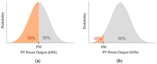
Figure 1.
P50 and P90 values represented in a normal distribution: (a) P50; (b) P90.
For PV system, which is widely used as a simulation program of solar energy systems [4], annual solar irradiance is assumed to follow the normal distribution in the P50/P90 calculation [5]. With the system advisor model (SAM) algorithm, two methods are used. Depending on whether or not the solar irradiance data distribution follows the normal distribution, P50/P90 is calculated from the cumulative distribution function (CDF) of the normal distribution if the solar irradiance data follow the normal distribution. Otherwise, P50/P90 is calculated from the empirical CDF, based on the assumption that all data occurrence probabilities are the same, by sorting the data in ascending order [3]. Furthermore, the results of a study performed in Spain, which exhibited the characteristics of annual global horizontal irradiance (GHI) in 13 locations in the USA, Europe, etc., reported that they followed the normal distribution [6].
However, real solar irradiance is a variable natural energy source that does not always follow the normal distribution, as shown in Figure 2. This graph shows the probability density function (PDF) of the normal distribution and probability histogram of the GHI on Mokpo over a 27-year period (1991 to 2017). Moreover, existing studies have also reported that the actual solar irradiance follow the asymmetric distribution rather than the normal distribution [1].
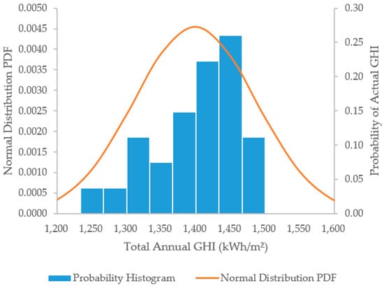
Figure 2.
Probability density function (PDF) of the normal distribution and probability histogram of the global horizontal irradiance (GHI) in Mokpo, Korea.
This study calculated the P50/P90 PV power potential from the skew-normal distribution, whereby skewness was applied to the normal distribution rather than assuming that the probability was the same, after sorting the data in ascending order if the solar irradiance simply did not follow the normal distribution.
In previous studies, the skew-normal distribution was found to be ideal for presenting appropriate models of real data that did not follow the normal distribution. Thus, a large number of studies on the application of the skew-normal distribution have been conducted [7,8,9]. In particular, the authors of Reference [7] improved the predictability of probabilistic solar irradiance using Bayesian model averaging (BMA), to which the skew-normal PDF was applied using the ensemble technique in Singapore. Moreover, when producing a daily solar irradiance using the CLImate GENerator (CLIGEN) model for regions in China, the model’s performance was improved by adding a skew coefficient to the normal distribution [9]. In addition, a study on daily solar irradiance modeling was also conducted based on various distributions in a tropical climate in France and Nigeria [10,11,12].
In this paper, four cities in Korea, which is located in the mid-latitude temperate zone and has four distinct seasons (spring, summer, autumn, and winter), were targeted to apply the normal distribution, skew-normal distribution, and empirical cumulative distribution, from which the P50/P90 PV power potential was calculated and the results were compared. The Jarque–Bera test was used as the goodness-of-fit test to determine whether solar irradiance data followed the normal distribution, and the AICc was used to determine which method produced a better result between normal and skew-normal distributions.
2. Research Area and Data
2.1. Research Area
As shown in Table 1, the average GHI value from 9 a.m. to 5 p.m. during the period 1991–2017 was calculated, and the result showed that the average GHI in Daejeon and Mokpo was highest at around 0.40 kWh/m2 among four cities, and that of Seoul was the lowest at 0.34 kWh/m2. Figure 3 shows the GHI map at four cities during the period 2013–2017.

Table 1.
City information.
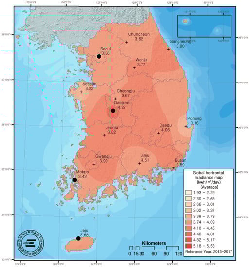
Figure 3.
GHI map of South Korea [13].
2.2. Data
This study used hourly GHI and air temperature data supplied by the Korea Meteorological Administration (KMA), as presented in Table 2. The data were produced using the Automatic Synoptic Observing System (ASOS), which comprises a pyranometer and an atmospheric temperature sensor. The GHI is stored every minute and observed once every second, thereby storing a mean solar irradiance of 60 observations. Each observatory stores the mean GHI per min (W/m²) data and the hourly cumulative GHI data (MJ/m²). A pyranometer from Kipp & Zonen CM21 was used. The air temperature sample was taken every 10 s using an electric resistance temperature sensor (100 Ω platinum resistance), and six recordings taken at 10-second intervals were averaged to obtain the minute-unit data. The hourly air temperature means the air temperature measured at 00 min of each hour [14,15].
Table 2.
Data information.
3. Methodology
As shown in Figure 4, whether the annual GHI data follow the Gaussian shape was determined by performing the Jarque–Bera test after inputting the hourly cumulative GHI data. Which distribution is more appropriate, i.e., which quality of the normal and skew-normal distribution is better, was determined using the AICc. Finally, the P50/P90 PV power potential was calculated using three methods, and their results were compared. In this paper, the simplest P50/P90 calculation method was used, and uncertainties such as data quality and climate change were not considered.
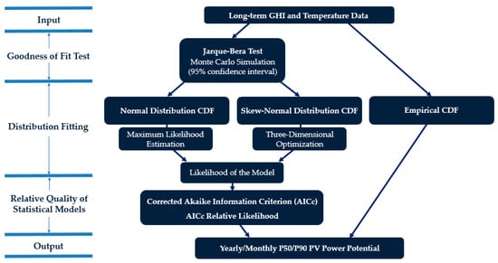
Figure 4.
Flowchart of P50/P90 photovoltaic (PV) power potential.
3.1. Three Distributions
3.1.1. Normal Distribution
P50 or P90 is calculated from the normal distribution CDF if the data distribution follows the normal distribution. The normal distribution is one of the continuous probability distributions, which is also called the Gaussian distribution. The shape is determined by mean μ and standard deviation σ. The mean and standard deviations were determined using the Maximum Likelihood Estimation (MLE). The P50 value means a mean value, and the P90 value can be calculated through the CDF of the normal distribution, such as Equation (1) [16]. The P90 value is obtained when .
- erf: Error function (also called the Gauss error function);
- μ: Mean;
- σ: Standard deviation.
3.1.2. Skew-Normal Distribution
This study attempted a new method using skew-normal distribution, in which skewness was applied to the normal distribution. This distribution was originally introduced by Azzalini (1985) [17], and its PDF is presented in Equation (2) [18].
In Equations (3) and (4), and refer to the standard normal PDF and CDF. α refers to the shape parameter, which has a range of . As shown in Figure 5, when α is a negative value according to the sign of α, it is skewed toward the right, but when α = 0, normal distribution, and when α is a positive value, it is skewed toward the left.
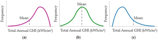
Figure 5.
Skew-normal distribution [19]: (a) Negatively skewed distribution; (b) Normal skewed distribution; and (c) Positively skewed distribution.
The CDF in the skew-normal distribution is presented in Equation (5), through which P50 and P90 were calculated. The scale parameter ω, mean ξ, and the shape parameter α have to be fitted to the data. This three-dimensional optimization problem was solved by creating a 3D parameter grid and testing the objective function at the grid points.
- T(h, α): Owen’s T function;
- ω: Scale parameter;
- ξ: Mean;
- α: Shape parameter.
3.1.3. Empirical Distribution
This method is used when the data do not follow the normal distribution, in which the data distribution is skewed when abnormal climate conditions, such as a blizzard or a volcanic eruption, occur. This method does not assume a specific statistical probability distribution, but the data are sorted in ascending order based on the assumption that each set of data occurs at the same probability to calculate P50 and P90. Table 3 presents the calculation process of the empirical CDF using the example of a four-point dataset.
Table 3.
Example of empirical cumulative distribution function (CDF) calculation.
3.2. Goodness of Fit Test
To determine whether the data follow the normal distribution, the Jarque–Bera test (usually shortened to just JB test) was used, as described above. Through the skewness of the Jarque–Bera test, the tendency of the data distribution shape to deviate toward either side of the mean can be found, and kurtosis can be used to determine the extent to which the data distribution shape is concentrated in the center. This can be expressed by Equation (6) [20]. The critical values and the p-value were calculated with a 0.05 significance level using the Monte Carlo simulation to accommodate the small sample size.
- n: Sample size;
- S: Sample skewness;
- K: Sample kurtosis.
3.3. Relative Quality of Statistical Models
Next, the relative quality of normal and skew-normal distributions were evaluated using AICc, as presented in Equation (7) [21,22,23], and an evaluation was conducted to determine which model was more appropriate. Since the relative information loss due to the model through the AIC value can be known, it can be estimated that the smaller the AIC value, the higher the quality of the model, which represents the data well. Because of the small sample size in this study, the AICc that best accommodated a small sample size was used.
- n: Sample size;
- k: Number of model parameters;
- L: Likelihood of model.
The difference between the two models can be found through the relative likelihood of the model, as presented in Equation (8). When selecting the high-quality model, it is better to choose a model whose relative likelihood is smaller. This value is between 0 and 1.
3.4. PV Power Potential
The PV power potential in this study was affected by the solar irradiance, temperature, and conversion efficiency of the solar cell array, as presented in Equation (9) [24]. This study exemplified a 3-kW small-scale PV power generation system, and the PV power potential was calculated using the target system, whose efficiency was 15% and area was 24 m2 array.
- : Conversion efficiency of the solar cell array (%);
- : Array area ();
- : Solar irradiance ();
- : Outside air temperature (°C).
4. Results and Discussion
4.1. Distribution Results
The AICc results showed that the information loss was relatively smaller when the normal distribution was selected, rather than the skew-normal distribution for Seoul, as presented in Table 4. However, the skew-normal distribution seemed more appropriate for Daejeon in the summer season (May to July) and the winter season (November to December). Similarly, for Mokpo and Jeju Island, the skew-normal distribution seemed more appropriate during May and November, and July or August. This result was obtained due to variables such as the rainy season and typhoon during the summer, when solar irradiance is high, and variables such as the heavy snowfall during the winter, when solar irradiance is low.
Table 4.
Distributions of four cities.
However, given that the range of the AICc relative likelihood was from 0 to 1, and that the difference between the two models increased as the AICc relative likelihood came closer to 0, the fact that the AICc relative likelihood was 0.3 on average indicated that there was no significant difference between the two models. Table 5 presents the annual and monthly AICc values in Daejeon. These values show how much data information was lost when fitting with each of the models. Figure 6 shows the PDF and the CDF of the normal and skew-normal distributions in Daejeon in December. The more appropriate distribution for Daejeon was the skew-normal distribution in December, in which the AICc value was 7.31 smaller than that obtained when the normal distribution was selected, and the difference between the two models was the largest among the four selected cities.
Table 5.
Annual and monthly Akaike information criterion (AICc) values in Daejeon.
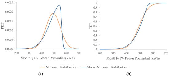
Figure 6.
PDF and CDF of normal distribution and skew-normal distribution in Daejeon on December: (a) PDF; (b) CDF.
4.2. Comparison of the Three Distributions
The difference between the three distributions was calculated based on the distribution recommended by AICc, as shown in Table 6. In the comparison, the area showing the greatest difference is Daejeon. If the normal distribution is the reference, the difference in the P90 value between the normal distribution and the empirical distribution is 4.37%. The next difference is Mokpo, which is the difference in the P90 value between the skew-normal and empirical distributions. Figure 7 shows the annual CDF graph of Mokpo’s annual PV power potential with three distributions. Based on the skew-normal distribution, which had a smaller AICc value than the normal distribution, the difference in the P90 value between the skew-normal distribution and the empirical distribution was 2.14%. In addition, there was a 0.54% difference in P90 between the skew-normal and normal distributions.
Table 6.
P90 and P50 PV power potentials of four cities.
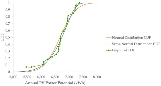
Figure 7.
CDF of the three distributions in Mokpo.
At P90, the average difference was 1.35% more than at P50. We further inferred that the reason for the difference in the P90 value is that it was less likely to occur than the average meaning of P50 and showed irregular characteristics.
The seasonal analysis of each region shows that Seoul, Daejeon, and Mokpo produced the highest generation in spring and the lowest in summer. However, in the case of Jeju Island, the lowest power potential was produced in winter. It is inferred that the main reason is the high temperature of Jeju Island in winter. Based on the data from 1991 to 2017, the average winter temperatures in the four regions were analyzed to be 7 °C in Jeju Island, while the other three regions were as low as −0.4 °C to 3 °C. According to the KMA, in January 2020, despite the winter season, the highest daytime temperature on Jeju Island was 23.5 °C, the highest temperature in January.
5. Conclusions
This study determined the best goodness-of-fit distribution when applying the normal, skew-normal, and empirical distributions based on the long-term solar irradiance database in four major cities in Korea, and compared the results after calculating the P50/P90 PV power potentials. In PVsyst, which has been widely used as a performance simulation program in existing solar energy systems, the normal distribution was assumed for annual solar irradiance data, and the P50/P90 values were calculated from the empirical CDF, whose data were sorted in ascending order based on the assumption that the probability of occurrence of all data was the same when the solar irradiance data did not follow the normal distribution in the existing SAM algorithm. However, this study presented a distribution, which was closer to the actual solar irradiance distribution mathematically, by applying the skew-normal distribution when the solar irradiance data did not follow the normal distribution. The Jarque–Bera test was used as the goodness-of-fit test to determine whether the solar irradiance data followed the normal distribution, while the AICc was used to determine which model produced a better quality result between the normal and skew-normal distributions.
- For Seoul, the result of AICc was obtained that the solar irradiance distribution was appropriate to the normal distribution. In contrast, for Daejeon, Mokpo, and Jeju Island, the skew-normal distribution was more appropriate during May and November, and July and August. The above results show that the appropriate distribution shape may differ depending on the region and season.
- Considering that the relative likelihood of the annual AICc was at least 0.3 or larger in the four regions, the quality of any single distribution model was not considered to be much better than the others. Information loss occurred upon selecting a single model, which showed that any one distribution would be appropriate for all. For the purposes of this study, only 27 samples were used, but at least 30 samples would be needed for model fitting [25]. Thus, the larger the number of samples, the lower the uncertainty will be [26]. Therefore, it is necessary to secure more annual solar irradiance data than the current study because this will make possible a more accurate model fitting.
- The results of the comparison of the P90 and P50 values when applying three distributions showed a larger difference in the P90 values than in the P50 values. The greatest difference between distributions was obtained in Daejeon, where the difference between the normal and empirical distributions was around 4.37%, followed by Mokpo, where the difference between the skew-normal and empirical distributions was around 2.14%.
- Based on the PV power potential, according to the seasonal analysis of the four cities, Jeju Island produced the lowest generation in winter, unlike the other three cities. In addition, in the previous study, when the PV power generation ramp analysis was conducted on 1450 PV power plants in Korea, the average ramp rate of Jeju Island was 11.5%, which was the most variable region in Korea [27]. Therefore, when the PV penetration level increased, especially in Jeju Island, it was necessary to thoroughly prepare for the worst case and take complementary measures when estimating backup facility capacity and reserve.
Projects that utilize solar energy, such as photovoltaics and concentrated solar thermal power, entail a certain degree of uncertainty, with the proportion attributable to solar resource uncertainty being around 5% to 17% [28]. This uncertainty could increase the project risk. As such, we hope that the results of this study could be used as the main data in an effort to reduce the degree of uncertainty in PV projects in Korea, where the proportion of PV power is being steadily increased by identifying the difference, although the difference was found to be just under 5% after applying a more realistic distribution to Korea, which has a continental climate.
Author Contributions
Conceptualization, software and formal analysis, S.Y.K. and B.S.; data curation, writing—original draft preparation, review and editing, S.Y.K.; supervision, G.J.; review and funding acquisition, H.-G.K.; funding acquisition, Y.-H.K. All authors have read and agreed to the published version of the manuscript.
Funding
The article processing charges (APC) was funded by the Korea Institute of Energy Technology Evaluation and Planning (KETEP) and the Ministry of Trade, Industry & Energy (MOTIE) of the Republic of Korea (No. 20194210200010).
Acknowledgments
This work was supported by the Korea Institute of Energy Technology Evaluation and Planning (KETEP) and the Ministry of Trade, Industry & Energy (MOTIE) of the Republic of Korea (No. 20194210200010).
Conflicts of Interest
The authors declare no conflict of interest.
Abbreviation
| AICC | Corrected Akaike Information Criterion |
| ASOS | Automatic Synoptic Observing System |
| BMA | Bayesian Model Averaging |
| CDF | Cumulative Distribution Function |
| CLIGEN | CLImate GENerator |
| GHI | Global Horizontal Irradiance |
| KMA | Korea Meteorological Administration |
| MLE | Maximum Likelihood Estimation |
| Probability Density Function | |
| PV | Photovoltaic |
| SAM | System Advisor Model |
References
- Kleissl, J. Solar Energy Forecasting and Resource Assessment, 1st ed.; Academic Press: Waltham, MA, USA, 2013. [Google Scholar]
- Cebecauer, T.; Suri, M. Typical Meteorological Year data: SolarGIS approach. Energy Procedia 2015, 69, 1958–1969. [Google Scholar] [CrossRef]
- Dobos, A.; Gilman, P.; Kasberg, M. P50/P90 Analysis for Solar Energy Systems Using the System Advisor Model. In Proceedings of the World Renewable Energy Forum, Denver, CO, USA, 13–17 May 2012. [Google Scholar]
- Lee, H.; Kim, S.; Yun, C. Comparison of solar radiation models to estimate direct normal irradiance for Korea. Energies 2017, 10, 594. [Google Scholar] [CrossRef]
- P50-P90 Evaluations. Available online: https://www.pvsyst.com/help/p50_p90evaluations.htm (accessed on 17 January 2020).
- Peruchena, C.M.F.; Ramírez, L.; Silva-Pérez, M.A.; Lara, V.; Bermejo, D.; Gastón, M.; Moreno-Tejera, S.; Pulgar, J.; Liria, J.; Macías, S.; et al. A statistical characterization of the long-term solar resource: Towards risk assessment for solar power projects. Sol. Energy 2016, 123, 29–39. [Google Scholar] [CrossRef]
- Aryaputera, A.W.; Verbois, H.; Walsh, W.M. Probabilistic accumulated irradiance forecast for Singapore using ensembel techniques. In Proceedings of the 2016 IEEE 43rd Photovoltaic Specialists Conference (PVSC), Portland, OR, USA, 5–10 June 2016. [Google Scholar]
- Na, J.; Yu, H. Saddlepoint approximation for distribution function of sample mean of skew-normal distribution. J. Korean Data Inf. Sci. Soc. 2013, 24, 1211–1219. [Google Scholar]
- Xie, Y.; Yin, S.; He, Q.; Liu, B.; Lin, X. Modifications of CLIGEN for simulation of daily solar radiation in China. ASABE 2011, 54, 451–459. [Google Scholar] [CrossRef]
- Soubdhan, T.; Emilion, R.; Calif, R. Classification of daily solar radiation distributions using a mixture of Dirichlet distributions. Sol. Energy 2009, 83, 1056–1063. [Google Scholar] [CrossRef]
- Linguet, L.; Pousset, Y.; Olivier, C. Identifying statistical properties of solar radiation models by using information criteria. Sol. Energy 2016, 132, 236–246. [Google Scholar] [CrossRef]
- Ayodele, T.R. Determination of probability distribution function for modelling global solar radiation: Case study of Ibadan, Nigeria. Int. J. Appl. Sci. Eng. 2015, 13, 233–245. [Google Scholar]
- Kang, Y.; Kim, H.; Yun, C.; Kim, C.; Kim, J.; Nho, N.; Kang, E.; Lee, J.; Chung, M.; Kim, H.; et al. Korea Atlas of New & Renewable Energy Resources, 3rd ed.; Korea Institute of Energy Research: Daejeon, Korea, 2019. [Google Scholar]
- Observation Policy Division. Partial Revision of Ground Weather Observation Guidelines; Korea Meteorological Administration: Seoul, Korea, 2011.
- Jee, J.; Kim, Y.; Lee, W.; Lee, K. Temporal and spatial distributions of solar radiation with surface pyranometer data in South Korea. J. Korean Earth Sci. Soc. 2010, 31, 720–737. [Google Scholar] [CrossRef]
- Normal Distribution. Available online: https://en.wikipedia.org/wiki/Normal_distribution (accessed on 17 January 2020).
- Azzalini, A. A Class of Distributions Which Includes the Normal Ones. Scand. J. Stat. 1985, 12, 171–178. [Google Scholar]
- Skew Normal Distribution. Available online: https://en.wikipedia.org/wiki/Skew_normal_distribution (accessed on 17 January 2020).
- University of Connecticut. Available online: https://researchbasics.education.uconn.edu/normal-distribution/# (accessed on 17 January 2020).
- Jarque-Bera Test. Available online: https://en.wikipedia.org/wiki/Jarque%E2%80%93Bera_test (accessed on 17 January 2020).
- Akaike Information Criterion. Available online: https://en.wikipedia.org/wiki/Akaike_information_criterion#How_to_use_AIC_in_practice (accessed on 17 January 2020).
- Hurvich, C.M.; Simonoff, J.S.; Tsai, C.L. Smoothing parameter selection in nonparametric regression using an improved Akaike information criterion. J. R. Statist. Soc. B 1998, 60, 271–293. [Google Scholar] [CrossRef]
- Burnham, K.P.; Anderson, D.R. Model Selection and Multimodel Inference A Practical Information-Theoretic Approach, 2nd ed.; Springer: New York, NY, USA, 2002. [Google Scholar]
- Zhao, J.; Wan, C.; Xu, Z.; Li, J. Impacts of large-scale photovoltaic generation penetration on power system spinning reserve allocation. In Proceedings of the 2016 IEEE Power and Energy Society General Meeting (PESGM), Boston, MA, USA, 17–21 July 2016. [Google Scholar]
- Wolf, E.J.; Harrington, K.M.; Clark, S.L.; Miller, M.W. Sample size requirements for structural equation models: An evaluation of power, bias, and solution propriety. Educ. Psychol. Meas. 2013, 76, 913–934. [Google Scholar] [CrossRef] [PubMed]
- Kim, S.; Lee, H.; Kim, H.; Jang, G.; Yun, C.; Kang, Y.; Kang, C.; Choi, J. A study on uncertainty to direct normal irradiance of typical meteorological year data. New Renew. Energy 2016, 12, 36–43. [Google Scholar] [CrossRef]
- Kim, S.; Kim, H.; Kim, B.; Kim, C.; Kang, Y.; Jang, G. Ramp characteristics of photovoltaic and wind power in south Korea. In Proceedings of the IEEE International Conference on Smart Cities: Improving Quality of Life Using ICT & IoT and AI, Charlotte, NC, USA, 6–9 October 2019. [Google Scholar]
- Schnitzer, M.; Thuman, C.; Johnson, P. Reducing Uncertainty in Solar Energy Estimates; AWS Truepower: Albany, NY, USA, 2012. [Google Scholar]


© 2020 by the authors. Licensee MDPI, Basel, Switzerland. This article is an open access article distributed under the terms and conditions of the Creative Commons Attribution (CC BY) license (http://creativecommons.org/licenses/by/4.0/).