Article

Modelling Future Agricultural Mechanisation of Major Crops in China: An Assessment of Energy Demand, Land Use and Emissions

1
Department of Chemical Engineering, Imperial College London, London SW7 2AZ, UK
2
Department of the Built Environment, School of Design, University of Greenwich, London SE10 9LS, UK
3
Instituto de Ingeniería, Universidad Nacional Autónoma de México, Mexico City 04510, Mexico
4
Department of Earth Science & Engineering, Imperial College London, London SW7 2AZ, UK
*
Author to whom correspondence should be addressed.
Energies 2020, 13(24), 6636; https://doi.org/10.3390/en13246636
Submission received: 22 November 2020 / Revised: 9 December 2020 / Accepted: 11 December 2020 / Published: 16 December 2020
(This article belongs to the Special Issue Changes of Global Energy Systems)

Abstract

:
Agricultural direct energy use is responsible for about 1–2% of global emissions and is the major emitting sector for methane (2.9 GtCO2eq y−1) and nitrous oxide (2.3 GtCO2eq y−1). In the last century, farm mechanisation has brought higher productivity levels and lower land demands at the expense of an increase in fossil energy and agrochemicals use. The expected increase in certain food and bioenergy crops and the uncertain mitigation options available for non-CO2 emissions make of vital importance the assessment of the use of energy and the related emissions attributable to this sector. The aim of this paper is to present a simulation framework able to forecast energy demand, technological diffusion, required investment and land use change of specific agricultural crops. MUSE-Ag & LU, a novel energy systems-oriented agricultural and land use model, has been used for this purpose. As case study, four main crops (maize, soybean, wheat and rice) have been modelled in mainland China. Besides conventional direct energy use, the model considers inputs such as fertiliser and labour demand. Outputs suggest that the modernisation of agricultural processes in China could have the capacity to reduce by 2050 on-farm emissions intensity from 0.024 to 0.016 GtCO2eq PJcrop−1 (−35.6%), requiring a necessary total investment of approximately 319.4 billion 2017$US.

1. Introduction

1.1. Emissions and Energy Use in Agriculture

Agricultural lands, due to their sheer proportion of overall land use and rigorous management, have a significant environmental impact on the earth’s carbon and nitrogen cycles. Houghton and Nassikas [1] estimated that since 1850, over 145 ± 16 GtC (µ ± 1σ) from biomass and soils has been emitted worldwide as a consequence of land-use and land-use changes. Deforestation due to crop and pastureland expansion accounted for 77% of the total emissions. Additionally, the sector is responsible for 2.9 GtCO2eq y−1 emissions of methane (CH4) due to manure management and enteric fermentation, and around 2.3 GtCO2eq y−1 of nitrous oxide (N2O) due to widespread use of fertiliser, increasing rice cultivation, manure inputs and soil degradation [2,3]. As a whole, the agriculture, forestry and land use sector is responsible for around 10–12 GtCO2eq y−1, which represents 25% of net anthropogenic greenhouse gas (GHG) emissions [4]. These estimates have an inherent high uncertainty and might vary considerably from study to study depending on the selected system boundaries.
Agricultural and land use emissions are especially critical for developing countries, where it is estimated that to cover the future food demand by 2050, productivity will have to increase to at least the double [5]. According to the Food and Agriculture Organization [6], current average daily energy food intake is about 11.6 MJ day−1 (2770 kcal day−1). Projections suggest that by 2050, due to an increase in population income, average daily intake could reach about 12.8 MJ day−1 (3050 kcal day−1) and 12.4 MJ day−1 (2970 kcal day−1) per person for developed and developing economies, respectively. Considering an increase in global population, it is estimated that the global food demand will increase by 60%–110% [5,7,8,9]. Moreover, it is expected that livestock production will increase driven by meat-based demand in developing countries. Thornton [10] expects that by 2050 food demand for livestock products will double in South Asia and sub-Saharan Africa, followed by South American and former-Soviet Union countries, while developed OECD countries will experience minimal change. In the case of China, He et al. [11] projects that with current diet patterns, by 2032, demand for land and water could increase around 14%; however, if recommended nutrition is followed, it is expected that China’s existing land would be insufficient to meet future demand, especially if appropriate measures and technological change is in place. If current trends of food production are kept (by intensification in developed economies and land clearing in developing economies), about 1 Gha of land would need to be cleared by 2050 for agricultural purposes only [7]. This represents emissions of about 3 GtCO2eq y−1 and 250 Mt y−1 of Nitrogen (N) from land management only.
Depending on the country, agricultural direct energy demand is between 2–8% [6,12] of the country’s demand. If the entire food supply chain is considered, this means including inputs for food processing, manufacturing and transport, this figure could increase to up to 30% [13]. Globally, in 2014 the sector was responsible for the consumption of 8.2 EJ or 0.46 GtCO2eq y−1. The main energy sources were electricity and diesel, representing three quarters of the whole consumption (Figure 1). In the past, several authors have investigated the impact of energy-related greenhouse gas (GHG) emissions in the sector [14,15,16,17,18,19,20]. Robaina-Alves and Moutinho [21] and Li et al. [22] found that two main cost-efficient paths exist to reduce sectoral emissions: (i) increase use of improved machinery (efficiency) and farming practices and (ii) promotion of production and utilisation of renewable energy sources.

Energy Inputs in Agricultural Crops

The agricultural sector is being and will be even more affected by climate change: even in a 2 °C world, the chance of major heatwaves will go to 49% with risk for maize heat damage equal to 18%, compared to 5% chance in 1981–2010 [23]. Global and regional impacts of climate change at different levels of global temperature increase). However, it is still missing a framework encompassing energy, environmental, and economic aspects in a single tool supporting effectively policy decision-making in the field. In this respect, the lack of comprehensive datasets is worsened by high heterogeneity of the sector.
On the energy use accounting side, although national energy balances publish the amount of energy demand and related emissions in the agriculture sector, the lack of disaggregated data by crop type is the main problem for a reliable understanding of the sector’s dynamics. Researchers have tried to disaggregate the impacts on GHG emissions due to individual crops. For example, Woods et al. [24] described the importance of a precise analysis of agricultural products, especially if emissions are to be modelled. Camargo et al. [25] used the ’Farm Analysis Tool’ to compare direct energy use and emissions for different crops in the north-east of the USA. Similarly, Pimentel [26] analysed the required direct and indirect energy inputs for twelve different crops in developed and developing nations.
As each crop is characterised by specific farming practices and machinery, the lack of crop disaggregation in the statistics generate a huge variability also in the labour inputs. For example, employment from the agricultural sector could make up anywhere within 50% to 90% of the population in developing economies [27], represented mainly by small independent farming operations with variation due to factors such as weather, technology diffusion and other geographical factors [28,29]. This variability reflects differences between developed and developing countries. For example, it has been estimated that the average input of human labour in the USA is around 11.4 h ha−1, while in developing countries such as India and Indonesia are about 634 h ha−1 [26].
Overall, the lack of comprehensive databases limits the modelling capabilities and in turn limits agricultural energy policy design.

1.2. Agricultural Mechanisation

In the last century, mechanisation in developed economies has dramatically reshaped the agricultural landscape [30]. Farm mechanisation have also brought higher yields and lower demand for land at the expense of higher inputs in the form of fossil-based energy and fertilisers. As the sector is very sensitive to social impacts and energy prices, rising prices usually force producers to seek new technological advances or methods to stay competitive, especially for large farms. The sector is very sensitive to environmental and social impacts as well as energy prices. Population and demand increase, diet change behaviour, impacts of climatic variability and weather extremes and rising energy prices usually force producers to seek new technological advances or methods to stay competitive [31]. Effects are more relevant for large farms as they have a more flexible structure which enables them to respond to market dynamics faster [32].
Economic growth and the commercialisation of agricultural systems is leading to further mechanisation of agricultural systems in developing countries in Asia and Latin America [33]. Over recent decades and mainly due to the introduction of new technologies, yields for most crops have been increasing between 1–2% y−1 [6]. Nevertheless, it is likely that these rates will be reduced for the foreseeable future [5]. The FAO [6] forecasts that crop yields will continue to grow at an average rate of 0.8% y−1; this value is half compared to previous decades (1.7% y−1). In fact, the appropriate mechanisation planning and the use of improved and efficient machinery and farming practices have the potential to enhance crop productivity while reducing energy intensity, land use and related emissions [22,34]. For instance, the European Commission [35] has developed a series of 28 agri-environmental indicators. One of those, number 12 refers to intensification/extensification. This indicator not only showcases the current farming intensity and agricultural productivity of each country members, but also provides an index that could be used for planning for sustainable agricultural practices in the region as well as to show the potential future socioenvironmental impacts of the sector.
Many authors have tried to characterise a mechanisation index to define the level of adoption of agricultural technologies. Nevertheless, the definition of a mechanisation index remains highly uncertain due to the simplification of the agricultural production process and the impact of other biophysical factors such as weather, water availability and soil characteristics. Conforti and Giampietro [18] defined a mechanisation index based on output-input ratio of global crop production, which was then later used by Ozkan et al. [36] for Turkey. Later, Singh [37] proposed a mechanisation index based on the ratio of cost of use of machinery to the total cost of use of human labour, draught animals and machinery.
Mechanisation has mainly concerned land preparation [38,39], tractorisation [40] and harvesting practices (crop rotation management [41]), but also the integration of reforestation practices [42,43,44,45] and which have led to energy consumption reduction. Finally, for the case of China, for example, Yang et al. [46] investigated the rapid mechanisation diffusion in China in in the previous decade; they show a five-fold increase in horsepower stock for medium and large tractors, and 25-fold for small tractors. Considering farms of around 133 ha of size, the study shown that the implementation of mechanisation and tractorisation has allowed farms to reduce harvesting time to only 2–3 h per farm.

1.3. Agricultural-Based ESM and Relevance for Policy Makers

To properly implement any energy-related technological measure in the sector, a rigorous analysis must be undertaken by simulation models to estimate the projected value of technical advances that would aid in the implementation of informed decisions by key actors in the sector. Generally, the agriculture sector has been neglected in energy systems modelling (ESM) due its lack of adequate direct and indirect energy use and emissions data that could aid to better characterise production processes in the sector. The increased role of bioenergy in the last years has been the main reason that a handful of ESMs started to consider the agricultural sector in its modelling approaches [47]. The sector’s interactions with other energy vectors as well with ecosystems makes it important for the inclusion in climate change mitigation studies and policies. For example, important dynamics exist such as the indirect energy input from fertilisers and other agrochemicals as well as the amount of total emissions related to the entire food, forestry products and bioenergy production processes [48].
Walker [15] described a method for modelling integrated energy systems in agriculture. The modelling algorithm helped identify the different classes of an agricultural process (including the material’s transformation, transport and storage). Each class is also associated with a cost, which can be monetary, labour, energy or land. Uri [49] provided a model to address fuel substitution between alternative types of energy focusing in the US agricultural sector. The author found the responsiveness of the sector to fuel price change. Later, he provided similar studies focusing on sectoral price responsiveness on diesel, gasoline, LPG and natural gas [16,17]. More recently, some authors have linked energy system models and detailed agricultural modelling to provide answer to specific questions [50,51,52,53].
Daioglu et al. [54] used the IMAGE, a spatial model with the capability of determining supply and demand of biomass and bioenergy products and its potential effect on the wider energy system by 2050. The model has been used to determine the future share of bioenergy in a 1.5 °C scenario. Results show that biomass could represent up to 20% (180 EJ/year) of the global energy consumption; nevertheless, for this to be achieved significant improvement in agricultural production and land zoning is needed. Similarly, Wu et al. [55] estimated bioenergy potential under carbon constrained scenarios and societal transformation measures. The authors based the analysis using a Computable General Model combined with a spatial Land Use and Environmental model. Authors found similar results for bioenergy production (up to 200 EJ/year by 2050) to the previous paper, with supply prices between USD 5/GJ and USD 10/GJ.
Other efforts where the modelling of the agricultural sector is essential is on the water-food-energy nexus research area. For instance, Li et al. [56] develop a stochastic model to optimise irrigated agriculture. This allows policy makers to develop programmes to optimise land, energy and water resources while maximising environmental and economic benefits of the agriculture sector. Elkadeem et al. [57] presented a techno-economic optimisation analysis for renewable energy integration aiming at agriculture and irrigation electrification. This study has the ability to present different technological systems structure that minimise environmental impact and maximise economic returns.
While the ESMs which integrate the agricultural sector, have a simplified description of the mechanisation in terms of emissions, energy demand and land use for specific crop types, the agriculture-oriented models include specific crops [58] but lacks of the integration with the rest of the energy system. To the best of the authors’ knowledge, there is no ESM which integrates a technology-rich agricultural sector modelling with a dynamic modelling of the whole energy sector. This modelling approach guarantees a comprehensive assessment of the energy use, agrochemical demand, land use as well as the emissions associated to the agricultural sector.

1.4. Study’s Aim

The aim of the paper is to assess the potential decarbonisation in the agricultural sector by proposing a comprehensive methodology in which mechanisation levels diffusion interplays with food and feed demand. The methodology is based on a modelling framework, the MUSE-Ag & LU model [59] which belongs to the MUSE modelling suite [60]. The proposed approach allows us to model the cross-dependencies between (i) socio-economic development, driving an expectedly high growth in demand of agricultural commodities, (ii) the energy demand linked to the technology development in agriculture, as represented by mechanisation levels, low-carbon fuels, and agrochemicals demand, and (iii) the sector emissions.
In addition, this tool has the capability to model the techno-economics as well as the environmental benefits of mechanisation on the harvest of specific crops. The main difference of MUSE-Ag & LU with other agricultural energy models is that energy technologies in the sector are represented by different levels of mechanisation; therefore, the model is capable to model and inform future mechanisation adoption in the sector. The model is part of a broader ESM which considers all the sectors in the economy, providing straightforward connections to model the dynamics between agriculture and the rest of energy vectors in the wider energy system. To demonstrate the model’s capabilities, this study will focus on analysing the following: (i) future specific crop demand for maize, soybean, wheat and rice under different scenarios (such as low and high food and feed demand and population growth), (ii) modelling of mechanisation adoption, labour and necessary investment, and (iii) analysing energy demand, land use change and related emissions for the selected crops.
To demonstrate the applicability of the novel framework, China has been selected as case study mostly due to data availability from the FAO [6] and USDA [61]. Another reason for the selection has been due to their importance in global food production, the potential for modern agricultural mechanisation and the expected dietary increases for the population. According to the FAO [6], currently the average vegetable-based daily food production for China is 9.9 MJ day−1 (2382 kcal day−1), and 58.4 and 37.1 g day−1 for protein and fat, respectively. However, if feed demand is also considered, these figures would increase by 803 kcal day−1 or 25%. As comparison, the USA food production stands at stands at 11.3 MJ day−1 (2697 kcal day−1), with supplies of 39.8 and 93.9 g day−1 of protein and fat, respectively; if feed demand is considered, the total value would increase by 23%. Usually a low share in feed demand (>20%) can be related to ruminants-based production systems, while larger shares is due non-ruminants fed production systems. Additionally, Pradhan et al. [62] considers that for the case of China, if the expected diet changes projections take place, feed demand share could increase to 1203 kcal day−1, representing 33% of the crop production share.
The paper is organized as follows. First the advancement compared to the MUSE-Ag & LU is described. Secondly, an overview of the modelled scenarios is presented. Next, the paper showcases the results, followed by discussions and conclusions.

2. Materials and Methods

2.1. MUSE-Ag & LU Additions

The general MUSE framework aims to simulates future decarbonisation scenarios in regional energy systems [63]. The Agriculture and Land Use (Ag & LU) module [59] is a model within the MUSE framework [63]. MUSE-Ag & LU, similar to other demand sectors in MUSE (buildings, transport and industry), contains investment decisions, as well as energy technologies representation with a particular land-use oriented modelling approach. Furthermore, the model determines the impact of the sector on global warming, quantifying emissions due to direct and indirect energy use as well as land use management and land use change. In doing so, the model applies a bottom-up approach and assesses the effects of technology innovation. The model produces a time series of fuel, agrochemicals and land demand to meet four general agricultural services: (a) crops, (b) animal-based food, (c) forestry products and (d) bioenergy [59]. The model accounts for CO2 emissions linked with on-farm energy use as well as N2O emissions (e.g., from fertiliser utilisation) and CH4 emissions (e.g., from rice production or manure management). The Ag & LU module generic simulation framework and integration with MUSE is represented in Figure 2.
The model has been expanded to model specific agricultural crops. In this sense, demand projections are necessary. To cover this demand, new mechanisation technologies have been characterised using cluster analysis and optimisation techniques. It is to this mechanisation processes, that data on energy inputs, yields, fertiliser demand, costs and related emissions have to be defined.
The modelling approach proposed does not explicitly model regional soil, climate, and non-technological factors affecting farming practices, but uses crop yields as a proxy which reflect the abovementioned factors. Crop yields are based on datasets which reflect the variability of local soil, climate and farming practices at an aggregated level. This paper will focus on the land, energy, emissions, and cost implications related to four main crops. However, land implications include constraints which refer the use for animal food, forest-based products, and bioenergy.
The following subsections explain the main steps followed in the development of the model.

2.1.1. Crop Selection

Originally, MUSE-Ag & LU [59] only modelled four general agricultural services: (a) food crops, (b) meat-based products, (c) forestry products and (d) bioenergy. In ESMs this simplification is a common approach due to its low global share of direct energy consumption and related greenhouse gas emissions [59]. In this study, the expansion of food crops is suggested. Table 1 displays the top 6 crops by global production for China as well as for the USA for comparison purposes.
Although, sugarcane is the most produced crop is also very sensitive to temperature, humidity, and other factors that vary largely by country. Thus, food has been disaggregated into four crops: maize, wheat, rice, and soybeans, mainly because their price is highly correlated with oil prices [64]. In China, where these crops represent about 33% of Chinese crop production [6], this would potentially have higher implications on food security.

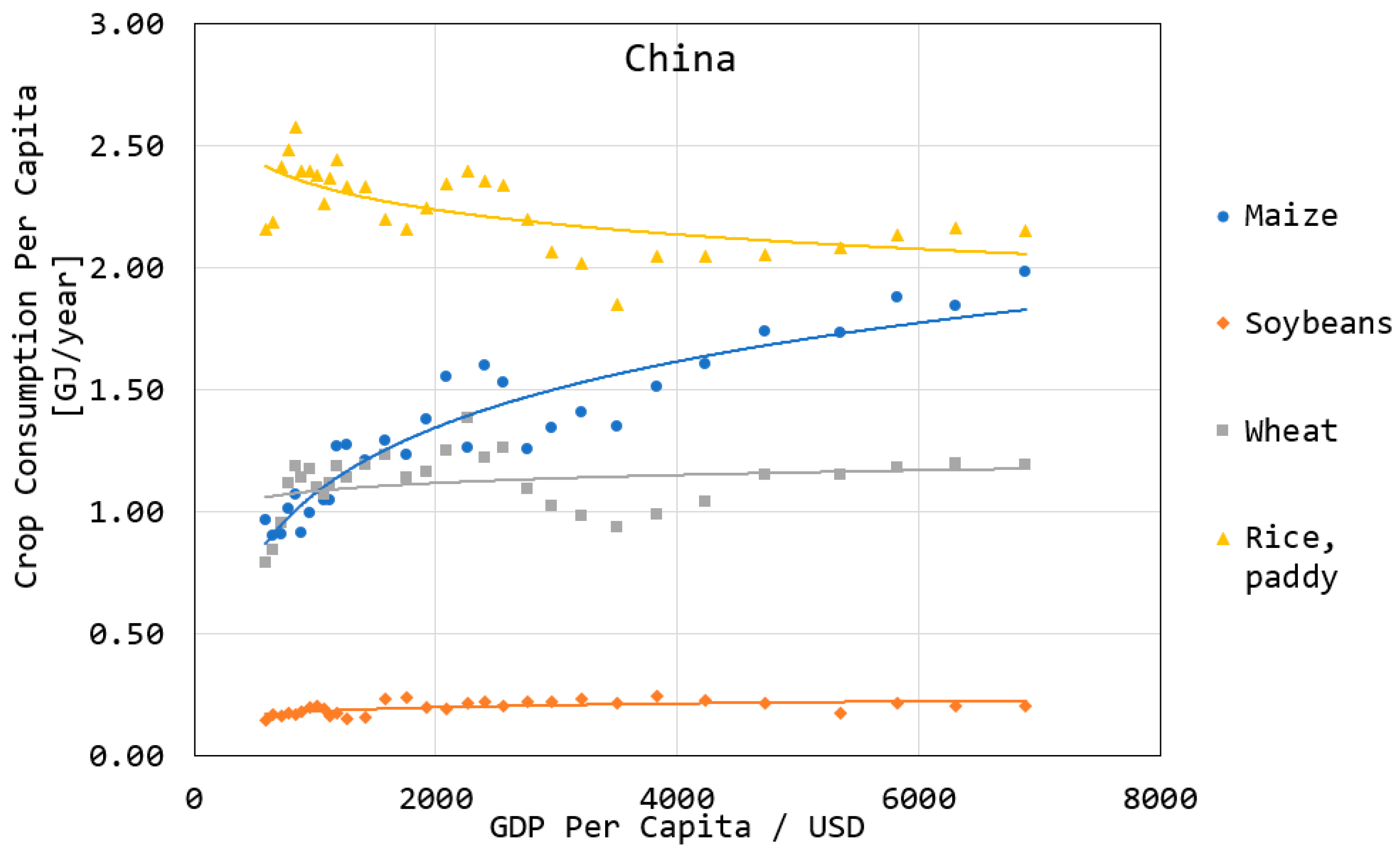
2.1.2. Crop Demand Projections

MUSE uses exogenously given macrodrivers (population and GDP) [27] to project future demands of services. Based on historical data, future crop demands are derived using regression models. As demand services are specified in Joules in MUSE, data on total calorie production per crop collected from the FAO [6] has been converted into Joules through the raw calorie density per crop type (Table 2).
Following, and similarly to van Ruijven et al. [65], linearised regression models have been used to identify that related economic activity (GDP per capita) to specific crops. In this case, four linear regression models were tested and implemented to forecast future crop demand:
Linear(L): C = a + b × GDPpc
Exponential(E): C = a × eb GDPpc
Semi-log(SL): C = a + b × ln(GDPpc)
Log-log(LL): lnC = a + b × ln(GDPpc)
In which a and b are constants estimated in the regression and serve as an input to the model. Both the R2 value and the root mean square error (RMSE) on per capita consumption values for all models are reported. The R2 values for the linear models are not all comparable, since some are for absolute consumption levels and others are for logarithmic values (ln(C)). Hence, the lowest RMSE model is selected for future predictions. The historical crop production per capita data, as well as the regressions tables highlighting the selected linear function for each crop model, are presented in Figure 3 and Table 3, respectively.

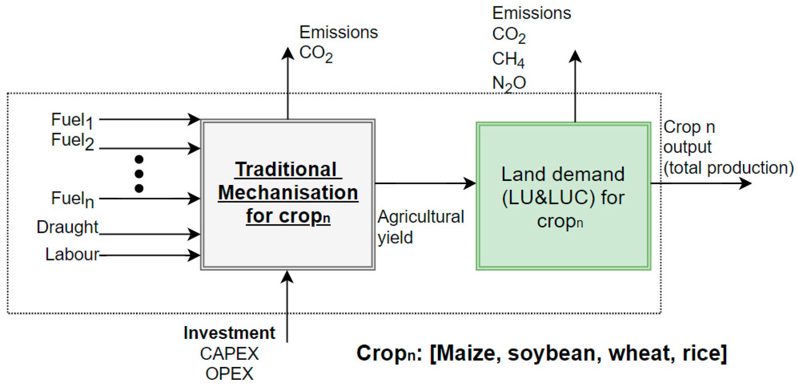
2.1.3. Mechanisation Levels
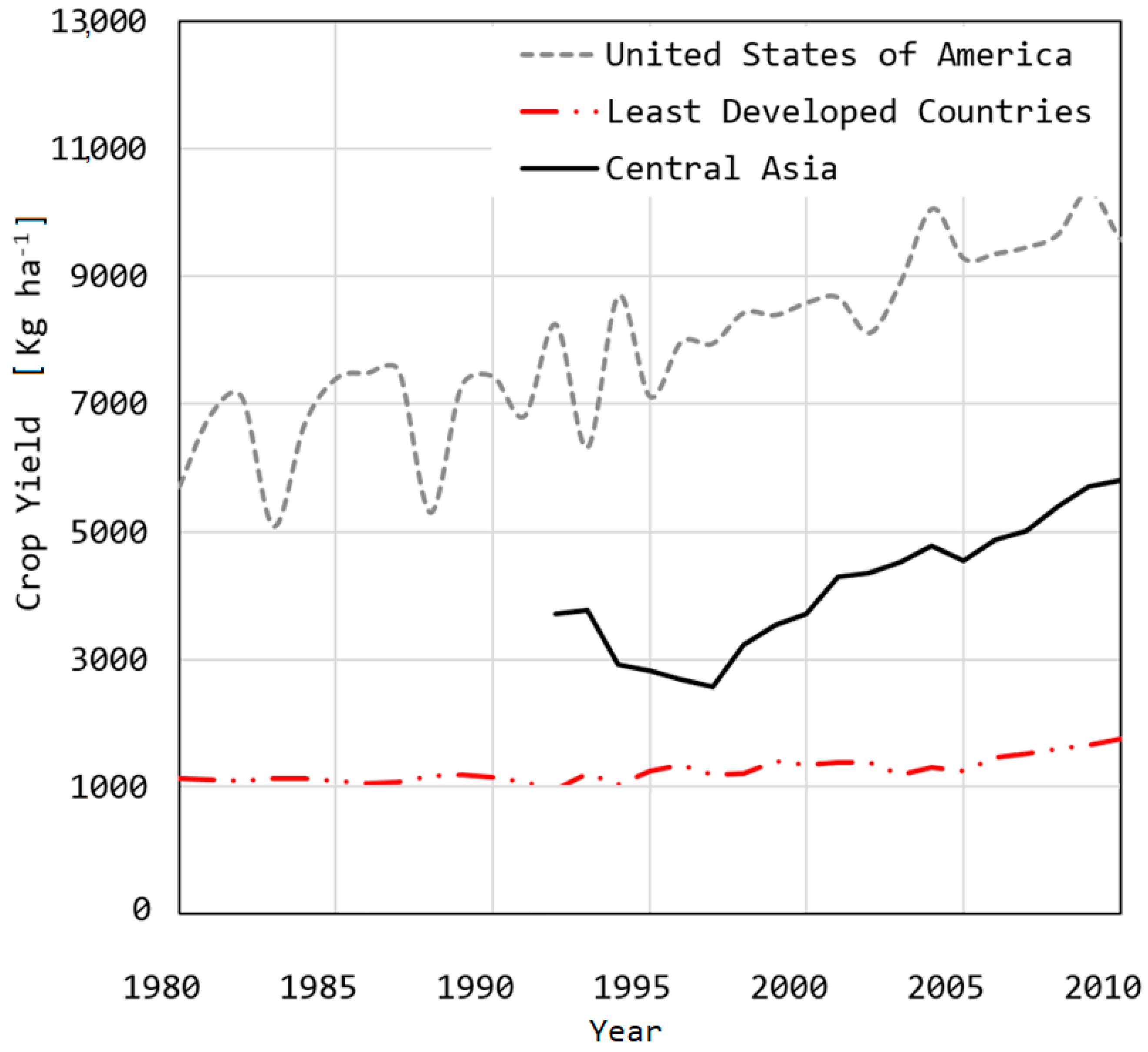
Similarly to [34], the model considers three levels of mechanisation: traditional, transitional and modern, with distinct inputs for fuel use, costs and production efficiencies. A basic representation of the agricultural mechanisation concept applied in the model is shown in Figure 4.
Traditional mechanisation considers both manual and some level of mechanised agriculture (e.g., tillers) with a minimum amount of direct and indirect energy. Transitional mechanisation presents mechanisation in some parts of the agricultural production chain. Tractors, tilling machines, mechanical heating/drying and irrigation using mainly electricity and other traditional fossil fuels are considered in this process. The use of fertilizers and agrochemicals is also common in this level.
Modern mechanisation, apart from a fully mechanised supply chain, it is considered technologically advanced equipment and other inputs in the form of irrigation water, fertilizers and pesticides. Additionally, an extra mechanisation level called “modern renewable” is represented. This level represents the data outliers or cutting-edge agricultural practices; therefore, it is assumed higher efficiency levels (input/output), a larger share of renewable energy and an optimised fertiliser utilisation.
Modern mechanisation levels (with high production rates) would come at much higher capital costs, representing how technical improvements are not attractive by default as farmers are al-ready operating in an area of decreasing marginal return. In MUSE, the demand for higher farm mechanisation emerges at the point when it becomes cost-effective for farmers to use it over other available options.
The identification of a mechanisation level and its characterisation requires the qualitative and quantitative assessment of a mechanisation index, and its impact on agricultural production (yield) and economic factors (cost of cultivation, deployment of mechanical power, agrochemical demand, animal power, etc.). The index should incorporate the significance and economic utility of using equipment with animate and electro-mechanical power for different farm operations in different crops. To generate the modelling technologies, a pre-processing approach is required and detailed in Appendix A. The characterisation of technologies has been obtained by applying the non-hierarchical method approach [18], based on cluster analysis of different countries at different levels of data observations from FAO [6].
To create technologies which adequately represent the heterogeneity of farming practices, mechanisation, and the relationship between climate, energy and agrochemical inputs and yields and mechanisation levels, cluster analysis has been conducted on national data. Among diverse economic variables, we have used GDP agricultural share (% GDPagr) aiming at providing a more robust insight into the agricultural technological development in a region. As described in [59] k-means clustering was used to reduce heterogeneity. For this, the following Hartigan–Wong minimization algorithm [66] was used:
W ( C k ) = x i C k ( X i   μ k ) 2
where X i is the actual cluster data, μ k is the cluster k data mean value. To identify the optimal amount of clusters, the Average Silhouette Method [67] was used:
S i = b i a i max ( b i , a i )
where b i and a i is the lowest average distance and average distance of data i with respect to the entire observations within one cluster, respectively.
Inputs for labour and draught are based in hours per crop output obtained from [37]. Table 4 presents the input values per mechanisation process for each analysed crop used in this study.

2.1.4. Crop Yields

A yield needs to be assigned for each mechanisation level for each crop. The crop yield has been obtained from historical data. For instance, Figure 5 displays the historical maize yields for three different regions of interest demonstrating different levels of agricultural development. As presented in [59], the ‘Least Developed Countries’ (countries considered have a %GDP agriculture share of above 16%) can be found to have yields between 1000 and 1400 kg ha−1; thus in this study, it has been assigned around 1200 kg ha−1 for traditional mechanisation for maize. On the other hand, the highest levels (represented by countries with a %GDP agricultural share of below 2%) present yields to around 8500 kg ha−1, which has been considered the yield for modern mechanisation processes The same approach was applied to the four crops assessed in this work. Yields values for each crop and mechanisation level is shown in Table 5.

2.1.5. Fertiliser Demand

Modern synthetic fertilisers are usually a combination of three main nutrients: nitrogen, phosphorous, and potassium (N, P2O5 and K2O). Levels of Nitrogen-based fertiliser per ton of production were obtained from FAO data [6] and USDA [61]. Observing the trends of global fertiliser use over the past century, a steady increase in total N-based fertiliser use for all crop types can be observed. This increase is linear for countries in time periods determined as traditional to modern but then lowers when a country reaches a cutting-edge level (above modern mechanisation levels). For instance, maize and wheat production in the USA, have experienced constant production growth and fertiliser use reductions. As time passes and yields increase with modern technologies, fertiliser application rates could become even more efficient. As Calaby–Floody [68] suggest, the inclusion of biotechnology and nanotechnology in the form of smart fertilisation with controlled nutrient release, could dramatically improve fertiliser efficiency.
To represents nutrient input for each mechanisation level and crop type historical data [61] a cluster analysis (using fertiliser input against crop yield) have been used. A full tabulated summary of fertiliser use for each level can be found in Table 6. Data analysis shows that the progression from traditional to modern is almost linear, but further modernisation to modern renewable lowers the demand of fertiliser, as application is starting to be optimised [6].

2.1.6. Integrating CH4 and N2O Emissions

FAO [6] data show that more than 70% of N2O emissions linked with farming are the result of synthetic and organic N fertilisers and crop residues. The sources of N2O are extremely varied for crop growth. To account for N2O emissions in the model, the following equation is used and highlights the different factors used to estimate direct N2O emissions [69]:
N2Otot,emm = (Fsn + Fon + Fcr + Fvol + Fleach) × EF1
where N2Otot,emm is total emissions by crop, Fsn is the N input from fertiliser use, Fon is the organic N applied as fertiliser (e.g., animal manure, compost, sewage sludge, rendering waste), Fcr is the above and below-ground N content of each crop, Fvol is N volatilization, Fleach is N from leaching processes, and EF1 is the emission factor per kg N fertiliser applied (assumed as 0.01 kg N2O-N). These concern all nitrogen-related processes, such as synthetic and organic fertilisation and crop residues. The sum of both direct and indirect emissions from these sources is then reduced to units of kt PJ−1 of crop produced for each mechanisation level (which uses different fertilisation amounts) and entered as a model input. For example, for transitional maize production, the Fsn = 215 kg ha−1; therefore, the associated emissions due to fertiliser input are considered at 2.15 kg N2O ha−1, which in turn converts to 0.027 kt N2O PJ−1 of maize.
Similarly, methane (CH4) emissions are considered due to their significance in the agricultural sector’s contribution to global GHG releases. All modelled values for GHG per mechanisation level are illustrated in Table 7.

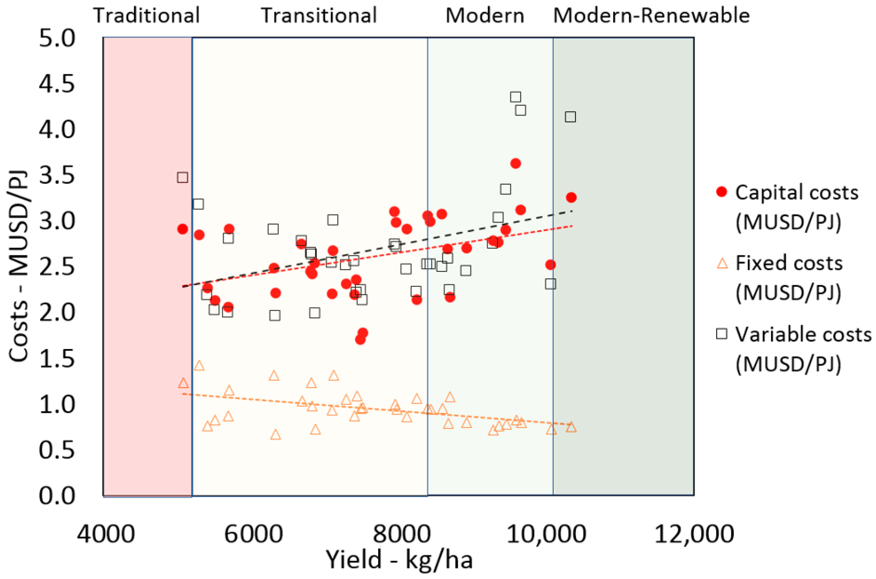
2.1.7. Techno-Economics of Mechanisation

MUSE-Ag & LU uses a bottom-up approach for technology characterisation, on which the net present value (NPV) is estimated to determine the investment in new technologies. In particular, new investments would favour technologies with a higher NPV.
For a detailed techno-economic characterisation of each mechanisation level, data on costs and return estimates from USDA [61] has been collected. The values are available in USD per planted acre. These values have been converted into USD per hectare using historic yield data [6] and then to USD per PJ y-1 to show unit price for installed capacity (also, USD values were scaled for inflation). The data has been plotted against the achieved yield (for instance, maize yields in Figure 6), and by locating the mechanisation level according to the yield, the capital, fixed and variable costs have been assigned. The obtained costs per mechanisation level for each crop are displayed in Table 8.

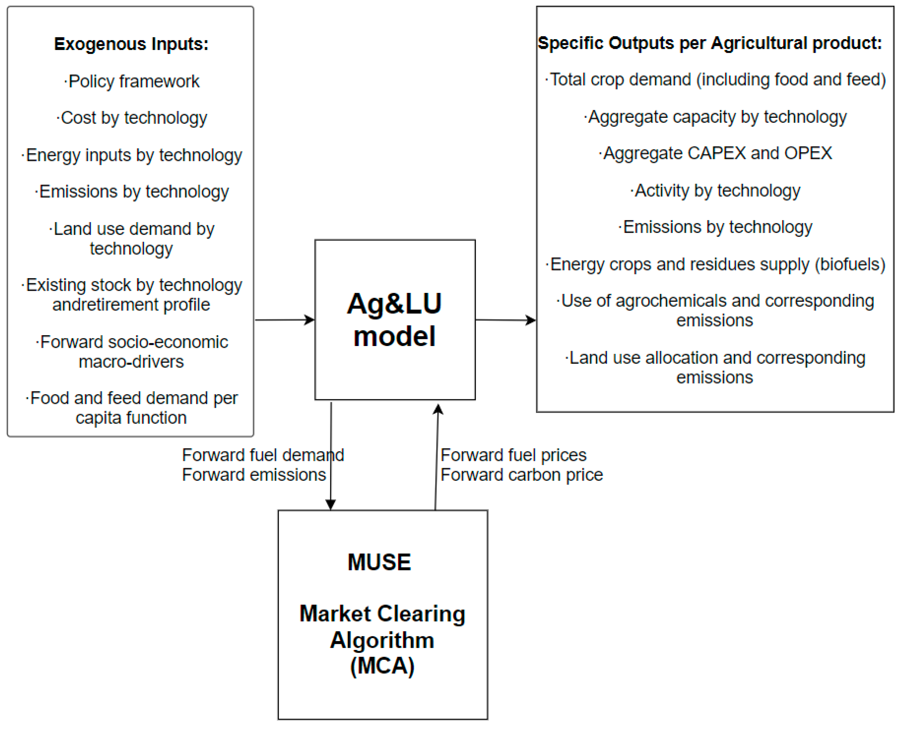
2.1.8. Model’s Inputs/Outputs

A summary of the main inputs used in the model as well as outputs provided by the model is shown in Table 9.

2.2. Calibration and Validation

Values on agriculture energy use, emissions, and land use have been calibrated using 2010 as a base year [6]. This year has been selected because of the existence and reliability of data for all the sectors as well as being a year without unusual political, economic or environmental circumstances. Additionally, the model has been validated by projecting values for 2010–2014 on food demand, fuel consumption, fertiliser demand, and emissions [6].
Due to lack of explicit data to account for the base-year installed capacities of the proposed mechanisation levels, a linear programming (LP) optimisation problem has been developed in the General Algebraic Modelling System [70] aiming at minimising the difference between actual and modelled sectoral emissions based on a set of constraints (share of mechanisation level and share of fuel per technology). To obtain modelled sectoral emissions, this pre-processing procedure considers the generated mechanisation levels by the LP, its fuel input share and the related emissions factors given by the [4]. By minimising the difference between modelled and actual emissions in the sector, the optimisation model is capable to calculate installed capacity of mechanisation levels per technology (t), crop (s) and region (r). The model mathematical formulation is presented in Appendix B. By solving this constrained optimisation problem, all structural alternatives are evaluated, and the programme identifies the best solution. The installed capacities by mechanisation level and its production shares by crop and by country obtained by the optimisation model are displayed in Table 10.

2.3. Scenarios

A set of three main scenarios have been developed to test the model:
  • Reference: To drive service demands, the SSP2 narrative, which describes a middle-of-the-road development for mitigation and adaptation [71], has been considered. The scenario considers a carbon price that is endogenously calculated by MUSE.
  • Low development: In this scenario, the SSP3 narrative, which describes a fragmented world, failing to achieve sustainable development goals, with little efforts in reducing fossil fuel utilisation and negative environmental effects has been considered. In this scenario, higher population growth (resulting in higher food and feed demand), as well as increases in technological costs and fuel prices, and a reduction in yield growth rates have been varied considering a 20% deviation from the Reference scenario. Additionally, no carbon price is considered.
  • High development: In this scenario, the SSP1 narrative, which describes a sustainable pathway, with constant efforts in reaching development goals and reducing dependency on fossil fuels mainly driven by rapid technological development, has been considered. In this scenario, lower population growth (resulting in lower food and feed demand), as well as reduction in technological costs and fuel prices, and increase in yields growth rates have been varied considering a 20% deviation from the Reference scenario. Apart from a carbon price for CO2 emissions, a specific tax has been imposed also on N2O and CH4. However, an imposed tax on these emissions needs to be weighted. Simulations have shown that a tax similar to the existing carbon level is too low, not only since N2O and CH4 are considerably more potent than CO2 but also due to the lower level of emissions; therefore, a low tax would be insignificant. On the other hand, applying a tax that reflects the global warming potential (e.g., N2O 298 times as strong as CO2) pushes technology levels back down to traditional agricultural practices and thus has an important impact on predicted land use and food security. At high GHG price rates, it is of interest for a farmer to revert to cheap, traditional technologies and use significantly more land to make up for the emissions costs. Therefore, compared to CO2 prices, a tax range between 0–300 times larger for N2O and 0–50 times larger for CH4 has been studied. After a sensitivity analysis, outputs suggest an optimal emission price of 10 times larger for CH4 and 25 times larger for N2O.
A linear decommissioning profile of existing technologies (existing mechanisation levels) has been applied. The imposed decommissioning profile implies that the capacity is totally renewed by 2040, 10 years ahead of the modelling horizon. Capital and operational costs of modern technologies are varied to understand the importance of price/subsidies in modern efficient technologies. Finally, yields annual growth rates are varied for both scenarios. A summary of each scenario is presented in Table 11.

3. Results

3.1. Reference Scenario

3.1.1. Mechanisation Adoption and Investment

The reference scenario estimates that by 2050, China’s overall demand (PJ y−1) for the analysed crops is projected to increase by 71%. Based on the modelling outputs, the technological shift in Chinese agriculture by 2050 is illustrated in Figure 7. The shift towards technologies with higher efficiencies is exhibited for maize, wheat and rice. The overall crop supply increases constantly until 2035 when population starts declining and crop production stabilises.
Overall, and considering all analysed crops, in the base year, “transitional” mechanisation is still responsible for 47.4% of the production, while “modern” and “modern renewable” for 44.5% and 5.3%, respectively. By 2050, “transitional” share decreases to 6.9%, overtaken by “modern” mechanisation with 61.9% of the production, followed by “modern renewable” with 31.1%. The forecast for soybean is rather different, but its low production compared to the rest of the crops, has barely any effect on the sector’s performance. Nevertheless, soybean results show a steep decrease reducing crop production as GDP per capita improves. This is in line with data from the previous decade, where soybean reached a maximum production level of 17 Mt y−1 in 2004, followed by an average annual decrease rate of 2.7% y−1. The main reason behind this was due to an increase in imports from Brazil, USA and Argentina in the last two decades [6]. It is possible that the country has been replacing more of its soybean production with other higher value crops. Additionally, in the short term it is not expected for soybean to play an important role in biodiesel production as currently the feedstock for Chinese biodiesel is mostly based on cotton, rapeseed and Jatropha [75].
In terms of investment and operational costs, the model suggests a necessary expenditure of around 319.4 billion 2017US$ by 2050, each crop requiring the following investment share: rice, 38.2%; maize, 35.3%; wheat, 25.2%; and soy, 1.3%. Modern technologies across the analysed crops would be responsible for around 95.8% of the total cost.

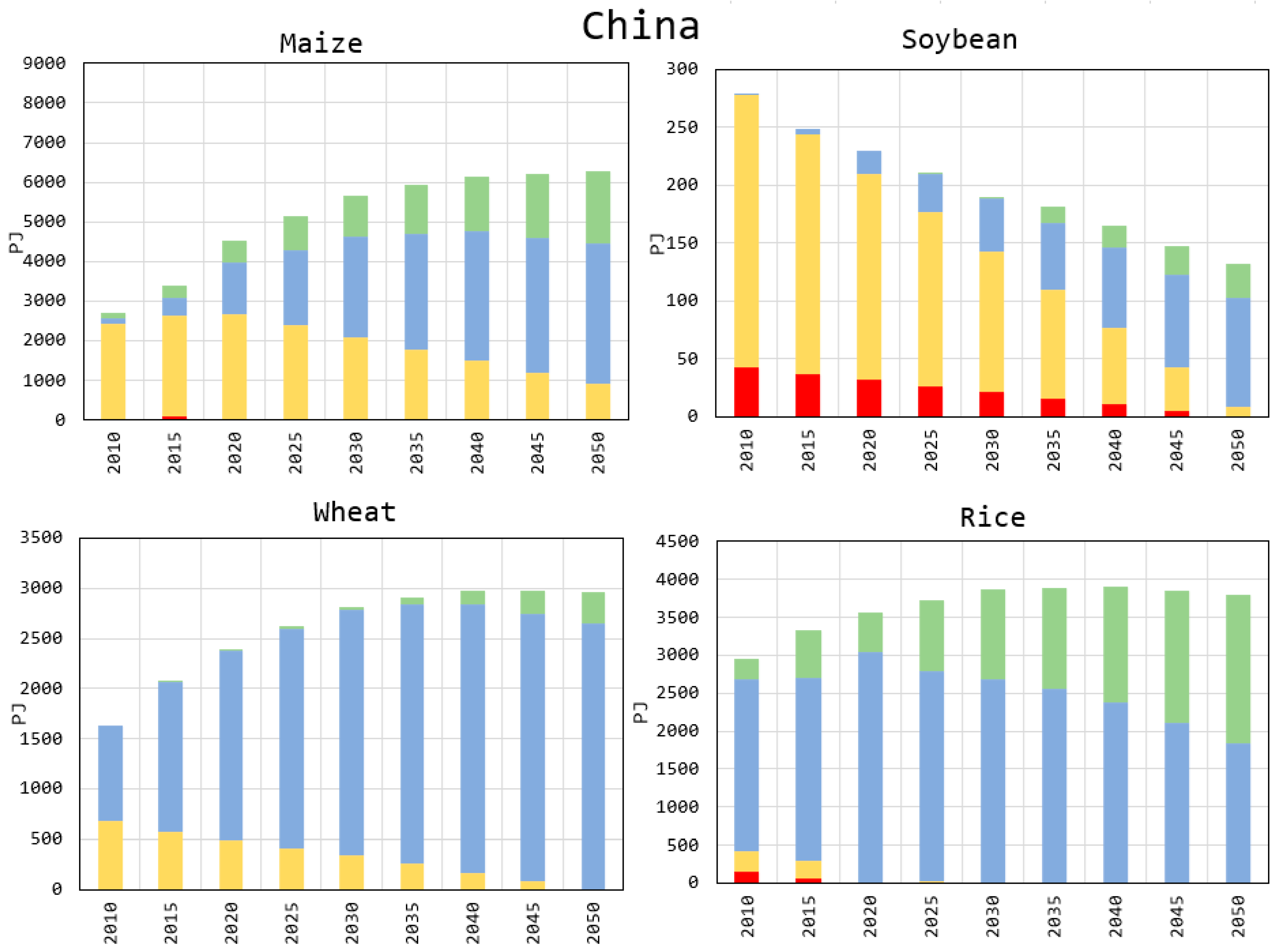
3.1.2. Energy/Fertiliser Demand and Related Emissions
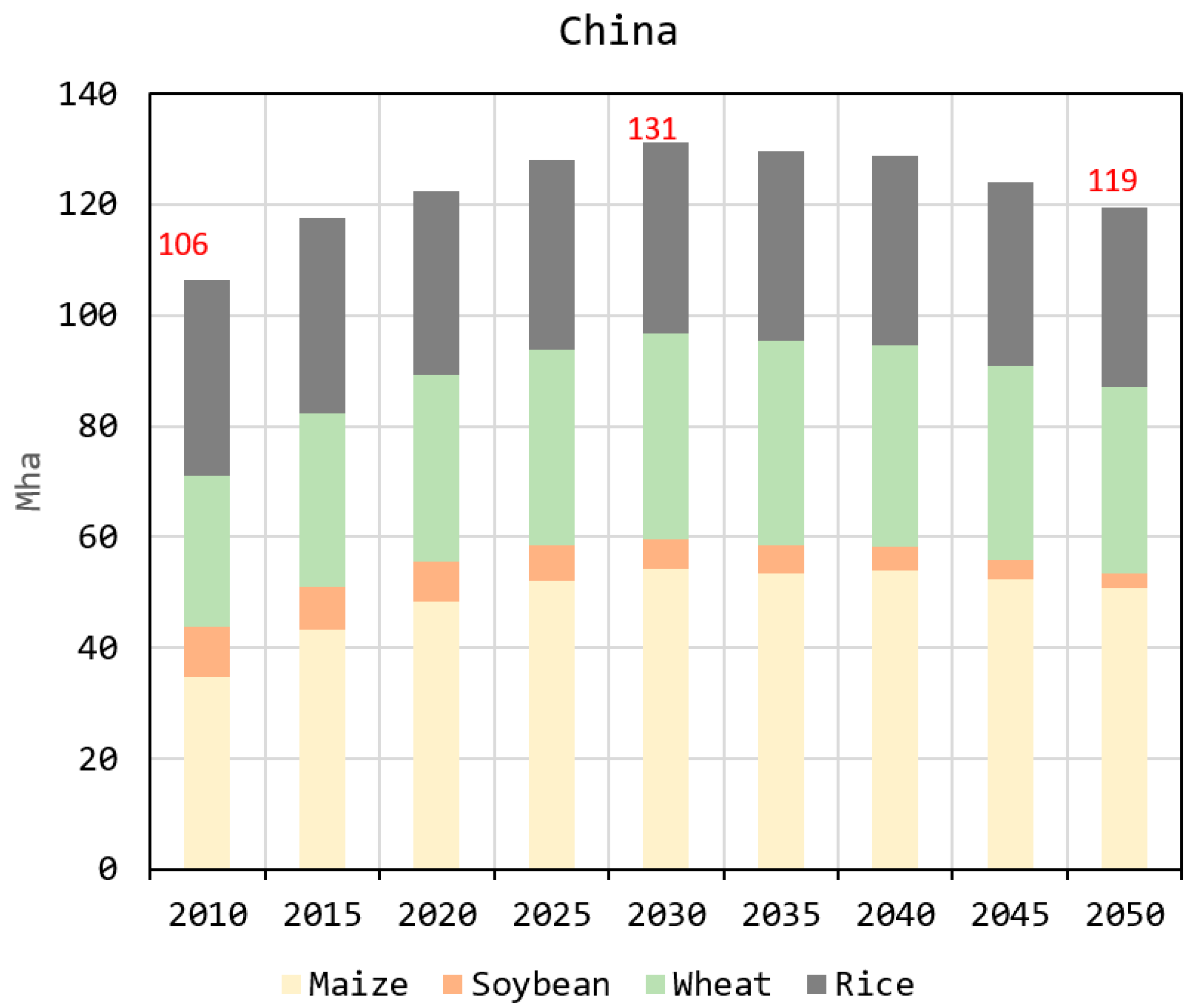
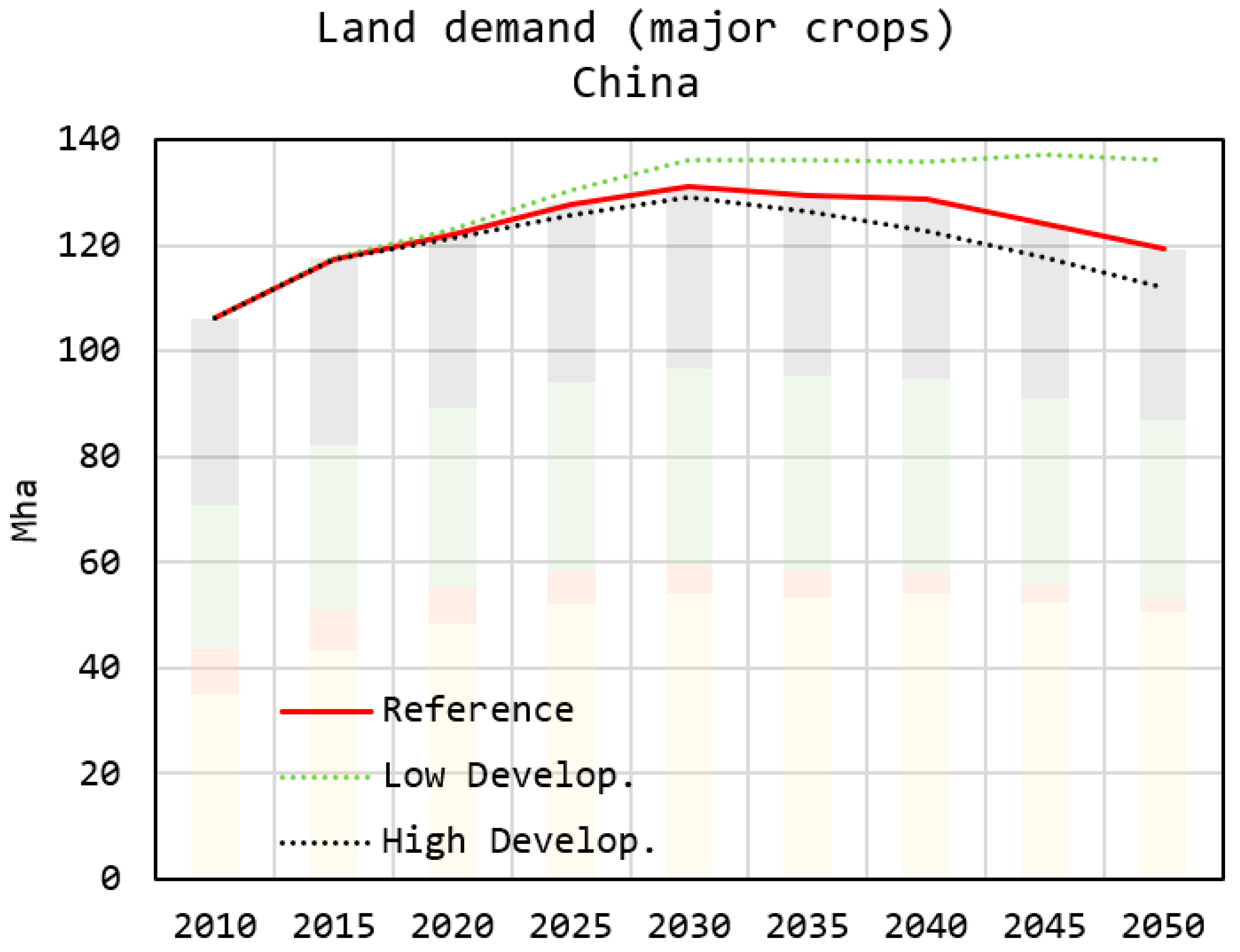
Table 12 shows the regional fuel consumption aggregated for the four crops. Outputs show two main drivers that impact the future projections: (i) the high prevalence of coal in the sector and (ii) the current low mechanisation levels and high labour/draught inputs. In 2010, the analysed crops demand 525 PJ y−1 of conventional energy (fossil and renewable), representing 39.1% of the total national agriculture energy use of 1342 PJ y−1 [6]. Demand is similar to countries such as the USA; however, for China, labour and animal input is higher, as it is estimated that 12.4 × 10⁹ h y−1 and 182.7 × 10⁹ h y−1 (or 88.9 million workers) comes from draught and labour work, a value estimated to be 40 times higher than in the USA.
Regarding to conventional energy sources, diesel, coal and electricity are the major fuels, representing 93.7% of the total fossil fuel inputs in the base year. By 2050, electricity and diesel retain their dominance of the overall fuel share, with coal reaching its maximum demand by 2025 and later being displaced by other energy sources used in modern technologies. Despite the growth in biofuels, their overall share remains small by 2050 (<5%), as “modern renewable” mechanisation is responsible of 31.1% compared to 61.9% of “modern” mechanisation that exclusively has fossil fuels as inputs. In terms of labour, it is expected a reduction of 69% reaching 56.6 × 10⁹ h y−1 or 27.9 million workers. For emissions, CH4 related emissions due to rice production represent the highest share, followed by N2O from fertiliser use and CO2 from fuel combustion. Overall emissions (CO2eq) grow by 11.9%, with N-related emissions with the highest increase (+46.1%), followed by CO2 (+30.2%). On the other hand, CH4 emissions due to rice cultivation are reduced by 8.6%, mainly due to the installation of more efficient technologies. In terms of emission intensity, this is reduced from 0.025 to 0.016 GtCO2eq PJcrop−1 (−35.6%).
N-based fertiliser demand in Mt is shown in Figure 8. For comparison, a projected demand for the USA has been included. In China, the consumption has been calculated at 16.2 Mt y−1, which represents 29.1% of the national demand. As seen, China’s fertiliser demand is higher than in the USA due to differences in production. This difference becomes more pronounced as the Chinese agricultural sector intensifies. By mid-century, China reaches 23.0 Mt y−1 of fertiliser demand (after peaking in 2040 to 24.2 Mt y−1).

3.1.3. Land Use

Figure 9 shows the land use modelling outputs for the four crops. In the base year, the analysed crops demand 106 Mha, with rice (33%) and maize (33%) as the as the largest croplands. Modelling results suggest that land demand will peak in 2030, increasing by 23%, to then shrink to 119 Mha by 2050, thus liberating land that could be used for other crops or for reforestation purposes. Apart from a reducing population at the end of the simulation period, the adoption of more efficient agricultural mechanisation processes with higher yields produces a decrease in land demand. The crop with the highest dynamism is maize, going from 35 Mha in 2010 to 51 Mha in 2050, while soybean gets reduced from 9 to 3 Mha.

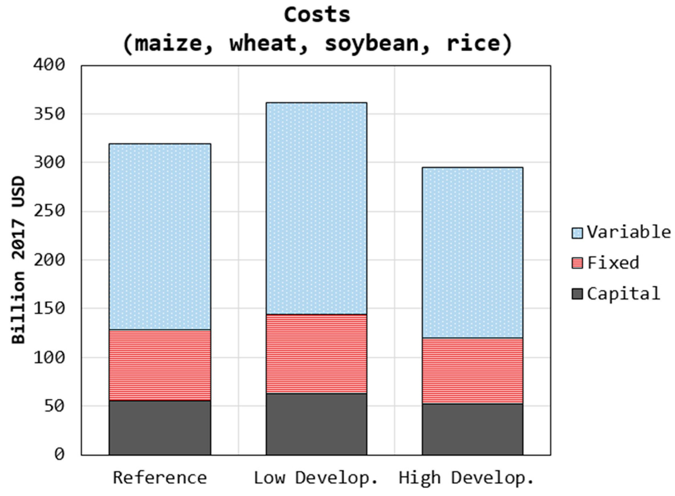
3.2. “Low” and “High” Development Scenarios

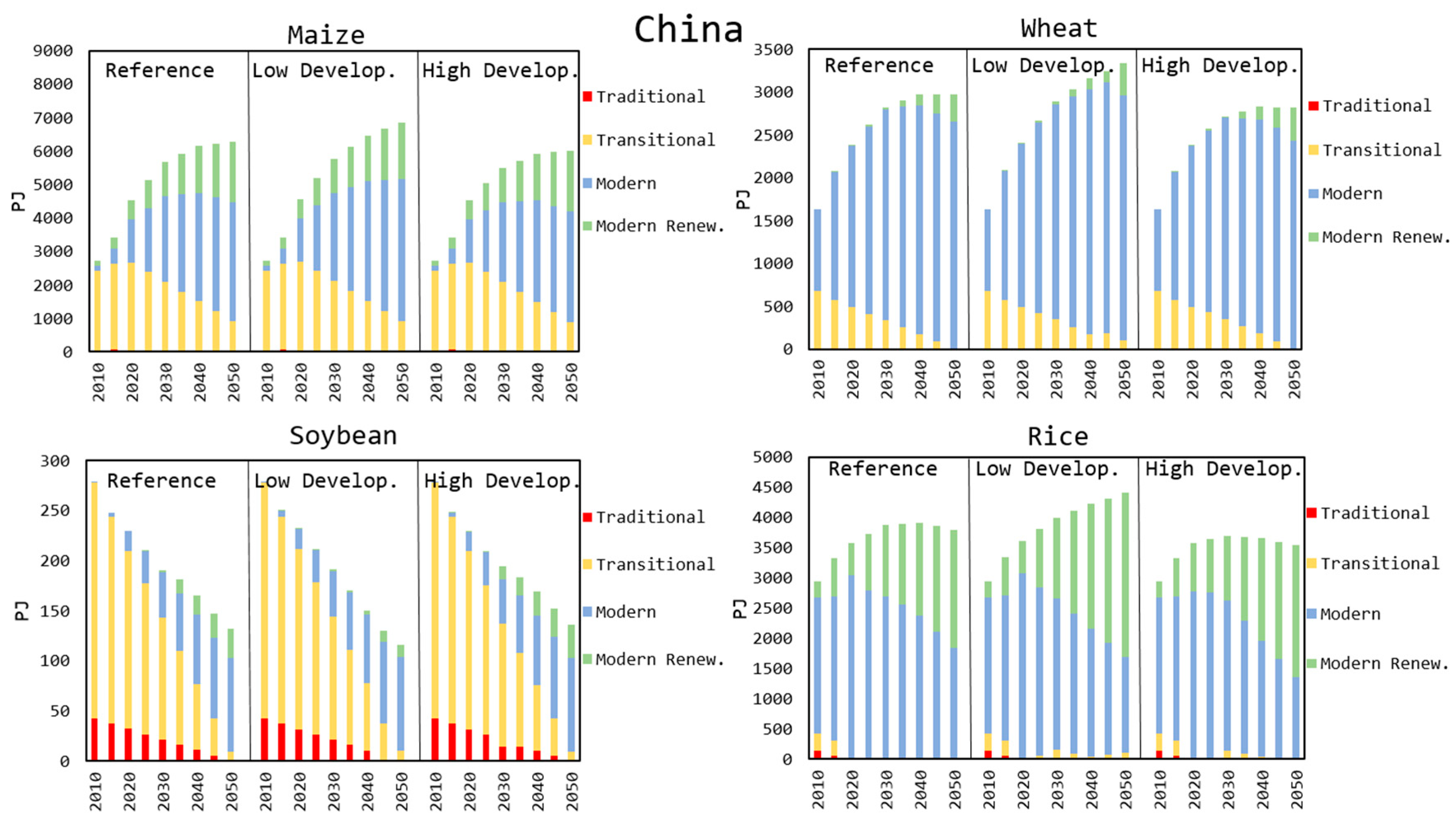
3.2.1. Mechanisation Adoption and Investment

In the “Low” development scenario, food demand increases due to higher population growth and per capita food intake. Additionally, it is expected that fossil fuels are not hit by carbon prices and advanced more efficient technologies become more expensive. Productivity diminishes due to the decreased investment in modern efficient technologies, as both the NPV differential between modern and transitional technologies is reduced. In the “High” development scenario, food demand reduces due to lower population growth and food intake per capita. Additionally, fossil fuels become more expensive as carbon tax is implemented (including CH4 and N2O), and advanced technologies become more competitive, as capital cost reduces and fuel cost becomes cheaper than the traditional options.
As illustrated in Figure 10, China would take up to 2040 to decommission transitional mechanisation, especially for maize and soybean. The outputs showcase the rate of adoption of modern technologies, where “modern” mechanisation almost overtakes by 2050 in all analysed scenarios. This result is expected as current trends in mechanisation diffusion in the country is following modernisation, thus moving to a slight increase in efficiency and renewable fuel share. However, modern efficient technologies with renewable energy share are not as predominant as fossil-based modern, being the latter the preferred choice for investors. In 2030, renewable energy starts to enter the sector, especially for maize and rice crops.
Sector mechanisation and intensification is expected for all analysed crops. For the reference case in China, in the base year, “transitional” mechanisation is still responsible of 47.4% of the production, while “modern” is responsible of 44.5%. By 2050, a shift is expected as “transitional” will only be responsible of 6.9%, while “modern” and “modern renewable” will be responsible for 61.9% and 31.1% of the total production. In the “High” development scenario, the “modern renewable” share increases to 35.2%.
The 2010–2050 investment required for the “Low” development scenario has been calculated at around 361.6 billion 2017US$, while for the “High” development at 295.4 billion 2017US$. Apart from a reduced installed capacity in the “High” development scenario which directly explains the lower costs, other important cost difference is found in the higher investment in “transitional” mechanisation processes in the “Low” development scenario (22.4 against 11.7 billion 2017US$), mainly due to lower fossil fuel prices and high cost of modern technologies. Figure 11 presents a cost comparison among the analysed scenarios.

3.2.2. Energy/Fertiliser Demand and Related Emissions

While in the “Low” development scenario, fuel use increases by 33.9% by 2050 (Table 13), in the “High” development scenario, a reduction of 34.1% compared to the reference is observed. For the reference and “Low” development scenarios, coal still represents the major energy source; however, in the “Low” development scenario that coal has a predominant share. Electricity and diesel are expected to still be major energy sources, but it is gasoline that has the highest growth rates regardless the scenario. Moreover, outputs show a low share of biofuels in future Chinese agriculture. However, if policies are made that promote the use of biofuels in the country’s energy system, this might slowly replace the demand of fossil fuels. For example, biodiesel or biomethane-fuelled agricultural technologies (e.g., farm machinery, farm equipment) could easily replace the demand of diesel in agriculture, which currently accounts for 8% of the national diesel consumption.
In terms of total emissions, the model shows a range between 191.0 Mt y−1 and 211.2 Mt y−1. Compared to the reference case base-year emission intensity of 0.025 GtCO2eq PJcrop−1, even a “Low” development would decrease the index to 0.019 GtCO2eq PJcrop−1, while a “High” development has the potential to reduce even further to 0.014 GtCO2eq PJcrop−1.
Finally, the most striking output is the reduction of labour demand. In the “Low” development scenario, labour is reduced by 61.1% (reaching 70.92 × 10⁹ h y−1 or 34.9 million workers), while in a highly mechanised sector, the reduction is in the order of 73.6% (employing 23.6 million workers). These values are important, as currently 20% of the Chinese workforce is employed in the agricultural sector [27]. To put this into perspective, the USA only employs 1.6% of its workforce for agricultural purposes.
Lastly, Table 14 shows the fertiliser demand for every scenario.

3.2.3. Land Use Change

Figure 12 illustrates the total land use demand projections for both scenarios compared to the outputs from the reference case. As previously discussed, for the “Low” development case, yields annual growth declines from 0.8% to 0.5%, thus putting more pressure on land. On the other hand, a “High” development scenario explores a yield growth increase to 1.3%.
Regardless of the scenario, it is expected an increase in land demand compared to the base year. However, the peak demand of land is expected between 2030 and 2035 for the reference case, in 2045 for the “Low” development, and in 2030 for the “High” development due to higher investment and more accessibility to modern technologies. At the end of the “High” scenario, land requirements for the four crops is expected to reach 112 Mha, compared to worst case of 136 Mha in the “Low” development. The “High” development scenario in turn could reduce emissions due to lower levels of deforestation and soil degradation.

4. Discussion

It is expected that developing economies will follow mechanisation diffusions similar to the past century trends experienced in developed economies. While some develop economies already have reached peak yields and technological diffusion in the majority of their crops, developing economies still have large potential for improvement, but also expect higher growth rates in food and feed demands due to the increase in population and per capita income. However, the greatest barrier for sustainable agricultural development is access to modern technologies, as most of the modern machinery is being developed in advanced economies thanks to larger and constant investment in R&D in the sector. As Safdar and Gevelt [76] discuss, developed economies are constantly strengthen its competitive advantage by combining investment and political lobbying. This has caused substantial barriers to local Chinese firms, that regardless of the state-support that the sector possesses, the technological gap of state-of-the-art machinery and processes between advanced economies and those from Chinese firms keeps widening.
Nevertheless, China keeps emphasising the development of the agricultural sector. The future development of the sector is not without related challenges. Among others, food demand security would require policies supporting smaller businesses and promoting advancements in production practices [77,78]. In addition to the economic implications, the introduction of advanced practices in agriculture becomes even more crucial when linked to emissions reduction from a perspective of low carbon transition.
Modelling outputs suggest that for all four crops analysed for the case of China, a shift towards modernisation is inevitable. The existence of some “transitional” agriculture is because in some rural regions, farmers are cultivating on marginal lands, where the access to more efficient technology might not be economically attractive. In this situation, it is the economic constraint that prevents the movement to the “modern” mechanisation levels, and not the lack of technological availability.
Analysis of variations over the reference scenario illustrate the dependence of the results on the made assumptions. In the “Low” development scenario, food demand is increased, fossil fuels are not hit by carbon taxes, and advanced technologies become more expensive. As expected, by mid-century, yields could decline in the range 10–14% for all crops compared to the reference scenario. This is due to the lower investment in modern technologies, as both the NPV differential between modern and transitional technologies is reduced, and the capacity gap is narrowed. On the other hand, in the “High” development scenario, food demand is reduced, fuels become more expensive, a tax on CH4 and N2O emissions is implemented, and advanced technologies become cheaper. In this case, yields improve in the range 16–24% for all crops compared to the reference scenario. In terms of direct energy use, despite the scenario, outcomes demonstrate that by 2050, electricity and diesel will still make up the largest portion of overall fuel use. However, if low development occurs in China, coal could still have a high share by 2050, hampering the national efforts to reduce economy-wide emissions.
The “High” development scenario shows a dramatic uptake of modern technologies in 2040—precisely when the current traditional and transitional technologies are fully decommissioned. It would be highly beneficial if policies promoting an early retirement of the existing technologies, when capital costs are outweighed by running costs, were put in place, accelerating decommissioning, namely if the resultant increase in capital costs is outweighed by the decrease in running costs.
Carbon taxes can have a significant impact on resource use and emissions. However, countries and relevant organisations are recommended to properly balance these taxes and subsidies. In the 2050 horizon, an optimal methane tax for controlling rice field emissions was observed at around USD 500/ton CH4, specifically for Chinese agriculture, contributing to around 20.1% emission reduction compared to the base case. Due to the extremely high emissions linked with permanently flooded rice fields, the pathways to reduce these emissions focus mainly on reducing the flooded period as much as possible, close control of water levels on fields, new seeding techniques, and/or sequentially managing wetting and drying of patties to prevent methane build-up [79]. Erda et al. [80] investigated potential carbon reduction options in the Chinese agriculture sector. The author found a potential reduction of 4–40% of CH4 emissions from better practice in rice, ruminants and animal waste, as well as reductions of 20% of N2O from micro-dosing fertilisation.
New land use techniques such as precision agriculture [81], i.e., any form of agriculture that changes conventions by utilizing new technologies, are expected in the future. As Stafford [82] suggests, precision agriculture has the potential to reduce environmental impacts by providing better crop and land management while increasing economic returns, thus providing a stronger market. In the methodology, it was highlighted that fertiliser use and its subsequent emissions incur high investment and pollution costs. The emergence of precision agriculture and the optimised outputs it promises are, therefore, of high interest for policy makers. Considering the already high yields achieved by farms in some countries, it is reasonable to assume that when this technology is made globally available, a high increase in application efficiency could be observed. Although not analysed in this study, diet changes towards less meat-based products (which in turn would reduce feed crop demand) combined with waste minimisation could be the most cost-effective measure aiming at reducing sectoral emissions to lower levels [83].

5. Conclusions

In this paper, a specific crop model for the agricultural sector integrated in an energy systems model has been proposed. This study proposed a simulation framework capable of modelling the future energy use, production, fertiliser demand, land use and related emissions as a function of mechanisation diffusion for specific crops. Four main crops have been studied to demonstrate the model capabilities. The techno-economic inputs refined by crop type provided a deeper under-standing of the value of technological advances within the sector and their implication in the wider energy system and environment.
Agricultural and land use models are set to play a significant role in helping decision makers to make informed decisions to ensure a future for the energy system, farming and global food production in line with a sustainable development. Mechanisation planning allows for both a quantitative assessment of advancement and serves as a tool for analysis in countries where specific data are lacking.
The current study presents scenarios of mechanisation in agriculture using China as a case study, which represents about 20% of global crop production. The results obtained demonstrate the complex variations by crop in technology investment, yields, fuel use, land demand and GHG emissions. Additionally, it is expected that the energy demand in the sector will increase driven by projected higher food demand, especially if more efficient technologies are not deployed. This can be seen in the “Low” development scenario, where higher investments in “transitional” mechanisation processes instead of “modern” mechanisation have been found, mainly driven by lower fossil fuel prices and high cost of modern technologies. Although coal would remain as an important source for Chinese agriculture, there would be room for electrification in the sector. On the other hand, biofuels would merely increase their share from 0.5% to up to 4.4% by mid-century. Despite the increase in energy demand expected across scenarios, outputs suggest a reduction in sectoral emissions compared to the base year, mainly due to a larger share of renewable energy and more efficient use of fertilisers and land.
The model also revealed important socio-economic implications in the reduction in dedicated human labour. If the modelled trends of increased mechanisation are extrapolated to the entire sector [27], a reduction of up to 114.5 million workers by 2050 could be expected. A workforce that eventually would need to switch either the industry and/or the service economic sectors.
For future work, the characterisation of the majority of agricultural crops is envisioned, as well as the different types of animal-based food production, forestry products and energy crops. Additionally, we expect to integrate a spatially explicit model that will characterise land suitability based on several biophysical characteristics such as temperature, soil, or water availability, aiming at understanding its effects in crop productivity and reduce uncertainties in the outputs.

Author Contributions

Conceptualization, I.G.K. and S.G.; methodology, I.G.K.; software, I.G.K. and S.G.; validation, I.G.K., E.S. and M.T.; formal analysis, I.G.K., E.S. and M.T.; investigation, I.G.K., E.S. and M.T.; resources, A.H.; data curation, I.G.K., E.S. and M.T.; writing—original draft preparation, I.G.K.; writing—review and editing, I.G.K., S.G. and A.H.; visualization, I.G.K.; supervision, I.G.K. and A.H.; project administration, I.G.K and S.G.; funding acquisition, A.H. All authors have read and agreed to the published version of the manuscript.

Funding

This work was supported by the Natural Environment Research Council (NERC) with grant number: NE/N018656/1.

Conflicts of Interest

The authors declare no conflict of interest.

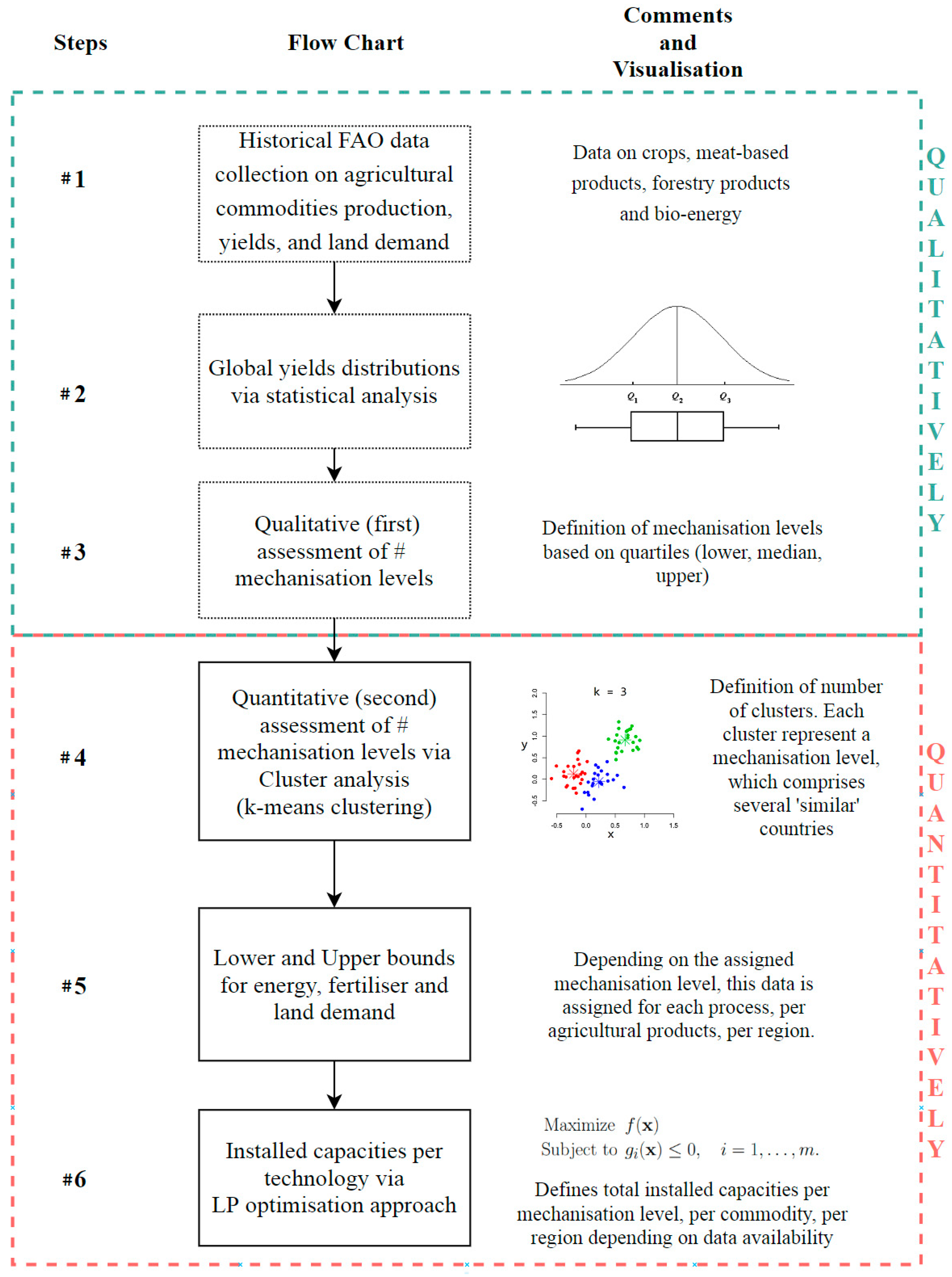
Appendix A. Framework to Characterise Agricultural Processes Based on Qualitative and Quantitative Approaches

A pre-processing six step approach combining qualitative and quantitative methods has been developed.
Step 1. Data on total production by country has been collected for the main agricultural commodities (crops, meat, and forestry products) and converted into energy units. Following, land use demands have been obtained for each agricultural commodity per region.
Step 2. Finally, after aggregating total production and land use demand per type of commodity, it is possible to obtain yields in energy units per area (PJ Mha−1). Distributions for each agricultural product on a global scale has been obtained.
Step 3. The outputs have been used to get a first qualitative definition of mechanisation levels depending on empirically observed yields (Step 3). In this case, as detailed in Section 2.1.3, three different levels of mechanisation have been defined using the quartiles calculated from the distributions. This technological classification is similar to mechanisation levels defined by the [6] (traditional, transitional, and modern) and by [84] (low level, intermediate level, and high level).
Step 4. To provide fuel share and land demand for each mechanisation process per agricultural product, a cluster analysis (k-means) has been implemented by locating countries with similar energy input/output ratios and yields characteristics per agricultural product.
Step 5. After grouping countries accordingly for each agricultural product, data on energy, fertiliser and land demand per unit product has been aggregated and probability distributions have been assigned to the different inputs to characterise those specific groups. Therefore, for each mechanisation level (traditional, transitional, and modern) and agricultural product (crops, meat, and forest) per region, fuel share, agrochemicals demand, yields and investment parameters have been defined with lower and upper bounds.
Step 6. To finalise the approach, it is necessary to calculate the total installed capacities by mechanisation level and by agricultural product for each region. For this, an optimisation problem (OP), based on integer linear programming (ILP) implemented in GAMS has been proposed, considering that only data on total sectoral energy demand and emissions by region are available.
Figure A1. Framework to characterise agricultural processes based on qualitative and quantitative approaches.
Energies 13 06636 g0a1

Appendix B. Mechanisation Installed Capacity Optimisation Model

To quantitatively characterise mechanisation levels into modelling processes, an optimisation problem (OP), based on linear programming (LP), has been implemented in GAMS [71]. The OP model aims to minimise the difference between real emissions and estimated emissions values for 2010, based on a series of constraints. As main modelling assumptions, different shares of mechanisation level are allocated to every region based on regional yields and the level of economic development. This means every country and region has some level of mechanisation level to greater or lesser extent. Depending on the region’s GDP agricultural contribution, different mechanisation share by level are characterize and used as bounds. Therefore, individual regions and crops would have to some extent a mechanisation level share. These bounds are shown in Table A1.
Table A1. Mechanisation share lower and upper bounds assumptions for different type of economies [59].
Type of EconomyTraditionalTransitionalModernModern Renewable
θtradθtranθmodθmodern
Least Developed (%GDPagr share > 0.16)50–70%10–20%10–20%1–2%
Emerging (0.02 < %GDPagr share < 0.16)10–20%50–70%10–20%3–5%
Developed (%GDPagr share < 0.02)10–20%10–20%50–70%5–10%
Along upper and lower bounds in other input parameters, the optimisation problem is formulated as follows:

Appendix B.1. Objective Function

The objective function minimises the difference between modelled emissions from real emissions in the sector:
m i n Z = r | Δ E r | + r , f | s l r , f |
where E r is the difference in emissions, while the sum of s l r , f represents the aggregation of all calculated slack variables.

Appendix B.1.1. Emissions Difference

The difference in emissions ( Δ E r ) can be obtained by:
Δ E r = R E M E
where R E represent the real emissions (obtained from FAO or IEA), and M E is the modelled emissions obtained by the model.

Appendix B.1.2. Emissions of the Model

The modelled emissions are calculated as follows:
M E = f , t C N r , f , t x F E f
where C N r , f , t is the fuel consumption for region r and technology t, and F E f is the emission factor for fuel type f.

Appendix B.2. Constraints

The OP is subject to the following quality and inequality constrains:

Appendix B.2.1. Mass Balance

First, the mass balance must be satisfied for every region, technology and agricultural service:
t T S s C P r , t > D M r , s   T S s
where CP refers to installed capacity, DM to service demand, r refers to region, t to technology mechanisation level, s to service type and T S s are the technology mechanisation levels available for service s.

Appendix B.2.2. Service Demand

The demand per service must be met by the sum of the share of production per mechanisation levels:
D M s = t θ s , t
where θ refers to the demand share covered by technology mechanisation level t.

Appendix B.2.3. Mechanisation Level Share

The share of production per mechanisation level ( θ s , t ) is obtained by dividing the demand met by specific mechanisation level over the total demand for service s:
θ s , t = D M s , t t T S s D M s     T S s
The share sum of mechanisation levels is constrained by the following equality:
θ t = θ s , t r a d + θ s , t r a n + θ s , m o d + θ s , m o d _ r e n = 1

Appendix B.2.4. Fuel Balance

The capacity per region and technology ( C P r , t ) is calculated from the total fuel consumption by technology in PJ multiplied by the technology yield or efficiency (PJ/PJ):
C P r , t = f C N r , f , t x   Υ t , s  
where f refers to fuel type, C N r , f , t to fuel consumption per region and technology, and Υ to efficiency of technology t for service s.

Appendix B.2.5. Fuel Constraint

The sum of fuel consumption by region and technology ( C N r , f , t ) is constrained by the total fuel demand in the region:
t C N r , f , t < ( F D r , f + s l r , f )
where F D r , f is fuel demand f in region r, and s l r , f is a slack variable added to make the problem feasible and fulfil the fuel constraints. The aim of adding a slack variable to an inequality constraint is to transform it into an equality constraint.
By solving the optimisation problem, all structural alternatives are evaluated, and the best solution is identified. The obtained capacities for each technology are used as an estimate of the base year stock.

References

  1. Houghton, R.A.; Nassikas, A.A. Global and regional fluxes of carbon from land use and land cover change 1850–2015. Glob. Biogeochem. Cycles 2017, 31, 456–472. [Google Scholar] [CrossRef]
  2. De Cara, S.; Houze, M.; Jayet, P.A. Methane and nitrous oxide emissions from agriculture in the EU: A spatial assessment of sources and abatement costs. Environ. Resour. Econ. 2005, 32, 551–583. [Google Scholar] [CrossRef]
  3. Reay, D.S.; Davidson, E.A.; Smith, K.A.; Smith, P.; Melillo, J.M.; Dentener, F.; Crutzen, P.J. Global agriculture and nitrous oxide emissions. Nat. Clim. Chang. 2012, 2, 410–416. [Google Scholar] [CrossRef]
  4. IPCC. Climate change 2014: Synthesis report. In Contribution of Working Groups I, II and III to the 5th Assessment Report of the Intergovernmental Panel on Climate Change; IPCC: Geneva, Switzerland, 2014. [Google Scholar]
  5. Ray, D.K.; Mueller, N.D.; West, P.C.; Foley, J.A. Yield trends are insufficient to double global crop production by 2050. PLoS ONE 2013, 8, e66428. [Google Scholar] [CrossRef] [Green Version]
  6. FAO. Faostat. 2017. Available online: http://www.fao.org/faostat/en/data (accessed on 15 January 2019).
  7. Tilman, D.; Balzer, C.; Hill, J.; Befort, B.L. Global food demand and the sustainable intensification of agriculture. Proc. Natl. Acad. Sci. USA 2011, 108, 20260–20264. [Google Scholar] [CrossRef] [Green Version]
  8. Valin, H.; Sands, R.D.; van der Mensbrugghe, D.; Nelson, G.C.; Ahammad, H.; Blanc, E.; Bodirsky, B.; Fujimori, S.; Hasegawa, T.; Havlik, P.; et al. The future of food demand: Understanding differences in global economic models. Agric. Econ. 2014, 45, 51–67. [Google Scholar] [CrossRef]
  9. Bodirsky, B.L.; Rolinski, S.; Biewald, A.; Weindl, I.; Popp, A.; Lotze-Campen, H. Global food demand scenarios for the 21st century. PLoS ONE 2015, 10, e0139201. [Google Scholar] [CrossRef]
  10. Thornton, P.K. Livestock production: Recent trends, future prospects. Philos. Trans. R. Soc. Lond. B Biol. Sci. 2010, 365, 2853–2867. [Google Scholar] [CrossRef] [Green Version]
  11. He, G.; Zhao, Y.; Wang, L.; Jiang, S.; Zhu, Y. China’s food security challenge: Effects of food habit changes on requirements for arable land and water. J. Clean. Prod. 2019, 229, 739–750. [Google Scholar] [CrossRef]
  12. IEA. International Energy Agency Statistics. 2017. Available online: https://www.iea.org/statistics/ (accessed on 30 January 2019).
  13. FAO. World Agriculture: Towards 2015/2030 an FAO Perspective; Earthscan Publications Ltd.: London, UK, 2003. [Google Scholar]
  14. Heichel, G.H. Agricultural production and energy resources: Current farming practices depend on large expenditures of fossil fuels. How efficiently is this energy used, and will we be able to improve the return on investment in the future? Am. Sci. 1976, 64, 64–72. [Google Scholar]
  15. Walker, L.P. A method for modelling and evaluating integrated energy systems in agriculture. Energy Agric. 1984, 3, 1–27. [Google Scholar] [CrossRef]
  16. Uri, N.D. Motor gasoline and diesel fuel demands by agriculture in the United States. Appl. Energy 1989, 32, 133–154. [Google Scholar] [CrossRef]
  17. Uri, N.D.; Gill, M. Agricultural demands for natural gas and liquefied petroleum gas in the USA. Appl. Energy 1992, 41, 223–241. [Google Scholar] [CrossRef]
  18. Conforti, P.; Giampietro, M. Fossil energy use in agriculture: An international comparison. Agric. Ecosyst. Environ. 1997, 65, 231–243. [Google Scholar] [CrossRef]
  19. Xu, B.; Lin, B. Factors affecting CO2 emissions in china’s agriculture sector: Evidence from geographically weighted regression model. Energy Policy 2017, 104, 404–414. [Google Scholar] [CrossRef]
  20. Ozturk, I. The dynamic relationship between agricultural sustainability and food-energy-water poverty in a panel of selected sub-Saharan African countries. Energy Policy 2017, 107, 289–299. [Google Scholar] [CrossRef]
  21. Robaina-Alves, M.; Moutinho, V. Decomposition of energy-related GHG emissions in agriculture over 1995-2008 for European countries. Appl. Energy 2014, 114, 949–957. [Google Scholar] [CrossRef]
  22. Li, T.; Balezentis, T.; Makuteniene, D.; Streimikiene, D.; Krisciukaitiene, I. Energy-related CO2 emission in European Union agriculture: Driving forces and possibilities for reduction. Appl. Energy 2016, 180, 682–694. [Google Scholar] [CrossRef]
  23. Arnell, N.W.; Lowe, J.A.; Challinor, A.J. Global and regional impacts of climate change at different levels of global temperature increase. Clim. Chang. 2019, 155, 377–391. [Google Scholar] [CrossRef] [Green Version]
  24. Woods, J.; Williams, A.; Hughes, J.K.; Black, M.; Murphy, R. Energy and the food system. Philos. Trans. R. Soc. Lond. Ser. B 2010, 365, 2991–3006. [Google Scholar] [CrossRef]
  25. Camargo, G.G.T.; Ryan, M.R.; Richard, T.L. Energy use and greenhouse gas emissions from crop production using the farm energy analysis tool. BioScience 2013, 63, 263–273. [Google Scholar] [CrossRef] [Green Version]
  26. Pimentel, D. Energy inputs in food crop production in developing and developed nations. Energies 2009, 2, 1–24. [Google Scholar] [CrossRef]
  27. World-Bank. World Bank Open Data. 2017. Available online: https://data.worldbank.org/ (accessed on 30 January 2019).
  28. Riahi, K.; van Vuuren, D.P.; Kriegler, E.; Edmonds, J.; O’Neill, B.C.; Fujimori, S.; Bauer, N.; Calvin, K.; Dellink, R.; Fricko, O.; et al. The shared socioeconomic pathways and their energy, land use, and greenhouse gas emissions implications: An overview. Glob. Environ. Chang. 2017, 42, 153–168. [Google Scholar] [CrossRef] [Green Version]
  29. Djanibekov, U.; Gaur, V. Nexus of energy use, agricultural production, employment and incomes among rural households in Uttar Pradesh, India. Energy Policy 2018, 113, 439–453. [Google Scholar] [CrossRef]
  30. Schmitz, A.; Moss, C. Mechanized agriculture: Machine adoption, farm size, and labor displacement. AgBioForum 2015, 18, 278–296. [Google Scholar]
  31. Olesen, J.E. Socio-economic Impacts—Agricultural Systems. In North Sea Region Climate Change Assessment. Regional Climate Studies; Springer: Berlin/Heidelberg, Germany, 2016. [Google Scholar] [CrossRef] [Green Version]
  32. Ren, C.; Liu, S.; van Grinsven, H.; Reis, S.; Jin, S.; Liu, H.; Gu, B. The impact of farm size on agricultural sustainability. J. Clean. Prod. 2019, 220, 357–367. [Google Scholar] [CrossRef]
  33. Appel, F.; Ostermeyer-Wiethaup, A.; Balmann, A. Effects of the German renewable energy act on structural change in agriculture—The case of biogas. Util. Policy 2016, 41, 172–182. [Google Scholar] [CrossRef]
  34. Baruah, D.C.; Bora, G.C. Energy demand forecast for mechanized agriculture in rural India. Energy Policy 2008, 36, 2628–2636. [Google Scholar] [CrossRef]
  35. European Commission. Eurostat: Agri-Environmental Indicators. Available online: https://ec.europa.eu/eurostat/web/agriculture/agri-environmental-indicators (accessed on 2 November 2020).
  36. Ozkan, B.; Akcaoz, H.; Fert, C. Energy input-output analysis in Turkish agriculture. Renew. Energy 2004, 29, 39–51. [Google Scholar] [CrossRef]
  37. Singh, G. Estimation of a mechanisation index and its impact on production and economic factors—A case study in India. Biosyst. Eng. 2006, 93, 99–106. [Google Scholar] [CrossRef]
  38. Mileusnic, Z.I.; Petrovic, D.V.; Devic, M.S. Comparison of tillage systems according to fuel consumption. Energy 2010, 35, 221–228. [Google Scholar] [CrossRef]
  39. Dalgaard, T.; Halberg, N.; Porter, J.R. A model for fossil energy use in Danish agriculture used to compare organic and conventional farming. Agric. Ecosyst. Environ. 2001, 87, 51–65. [Google Scholar] [CrossRef] [Green Version]
  40. Nkakini, S.O.; Ayotamuno, M.J.; Ogaji, S.O.T.; Probert, S.D. Farm mechanization leading to more effective energy-utilizations for cassava and yam cultivations in rivers state, Nigeria. Appl. Energy 2006, 83, 1317–1325. [Google Scholar] [CrossRef] [Green Version]
  41. Alluvione, F.; Moretti, B.; Sacco, D.; Grignani, C. EUE (energy use efficiency) of cropping systems for a sustainable agriculture. Energy 2011, 36, 4468–4481. [Google Scholar] [CrossRef]
  42. Veiga, J.P.S.; Romanelli, T.L.; Gimenez, L.M.; Busato, P.; Milan, M. Energy embodiment in Brazilian agriculture: An overview of 23 crops. Sci. Agric. 2015, 72, 471–477. [Google Scholar] [CrossRef]
  43. Garcia Kerdan, I.; Giarola, S.; Hawkes, A. Implications of future natural gas demand on sugarcane production, land use change and related emissions in Brazil. J. Sustain. Dev. Energy Water Environ. Syst. 2020, 8, 304–327. [Google Scholar] [CrossRef]
  44. Garcia Kerdan, I.; Giarola, S.; Jalil-Vega, F.; Hawkes, A. Carbon sequestration potential from large-scale reforestation and sugarcane expansion on abandoned agricultural lands in Brazil. Polytechnica 2019, 2, 9–25. [Google Scholar] [CrossRef] [Green Version]
  45. De Oliveira, L.L.; Garcia Kerdan, I.; de Oliveira Ribeiro, C.; do Nascimento Oller, C.A.; Rego, E.E.; Giarola, S.; Hawkes, A. Modelling the technical potential of bioelectricity production under land use constraints: A multi-region Brazil case study. Renew. Sustain. Energy Rev. 2020, 123, 109765. [Google Scholar] [CrossRef]
  46. Yang, J.; Huang, Z.; Zhang, X.; Reardon, T. The rapid rise of cross-regional agricultural mechanization services in China. J. Agric. Econ. 2013, 95, 1245–1251. [Google Scholar] [CrossRef]
  47. Wise, M.; Calvin, K.; Kyle, P.; Luckow, P.; Edmonds, J. Economic and physical modeling of land use in GCAM 3.0 and an application to agricultural productivity, land, and terrestrial carbon. Clim. Chang. Econ. 2014, 5, 1450003. [Google Scholar] [CrossRef]
  48. FAO. “Energy-Smart” Food for People and Climate; Food and Agriculture Organization of the United Nations: Rome, Italy, 2011. [Google Scholar]
  49. Uri, N.D. Energy substitution in agriculture in the United States. Appl. Energy 1988, 31, 221–237. [Google Scholar] [CrossRef]
  50. Elobeid, A.; Tokgoz, S.; Dodder, R.; Johnson, T.; Kaplan, O.; Kurkalova, L.; Secchi, S. Integration of agricultural and energy system models for biofuel assessment. Environ. Model. Softw. 2013, 48, 1–16. [Google Scholar] [CrossRef]
  51. Miljkovic, D.; Ripplinger, D.; Shaik, S. Impact of biofuel policies on the use of land and energy in U.S. agriculture. J. Policy Model. 2016, 38, 1089–1098. [Google Scholar] [CrossRef]
  52. Rochedo, P. Development of a Global Integrated Energy Model to Evaluate the Brazilian Role in Climate Change Mitigation Scenarios. Ph.D. Thesis, Federal University of Rio de Janeiro, Rio de Janeiro, Brazil, 2016. [Google Scholar]
  53. Al-Mansour, F.; Jejcic, V. A model calculation of the carbon footprint of agricultural products: The case of Slovenia. Energy 2017, 136, 7–15. [Google Scholar] [CrossRef]
  54. Daioglou, V.; Doelman, J.; Wicke, B.; Faaij, A.; van Vuuren, D.P. Integrated assessment of biomass supply and demand in climate change mitigation scenarios. Glob. Environ. Chang. 2019, 54, 88–101. [Google Scholar] [CrossRef] [Green Version]
  55. Wu, W.; Hasegawa, T.; Ohashi, H.; Hanasaki, N.; Liu, J.; Matsui, T.; Fujimori, S.; Masui, T.; Takahashi, K. Global advanced bioenergy potential under environmental protection policies and societal transformation measures. GCB Bioenergy 2019, 11, 1041–1055. [Google Scholar] [CrossRef] [Green Version]
  56. Li, M.; Fu, Q.; Singh, V.P.; Liu, D.; Li, T. Stochastic multi-objective modeling for optimization of water-food-energy nexus of irrigated agriculture. Adv. Water Resour. 2019, 127, 209–224. [Google Scholar] [CrossRef]
  57. Elkadeem, M.R.; Wang, S.; Sharshir, S.W.; Atia, E.G. Feasibility analysis and techno-economic design of grid-isolated hybrid renewable energy system for electrification of agriculture and irrigation area: A case study in Dongola, Sudan. Energy Convers. Manag. 2019, 196, 1453–1478. [Google Scholar] [CrossRef]
  58. Jones, J.W.; Antle, J.M.; Basso, B.; Boote, K.J.; Conant, R.T.; Foster, I.; Godfray, H.C.J.; Herrero, M.; Howitt, R.E.; Janssen, S.; et al. Brief history of agricultural systems modelling. Agric. Syst. 2017, 155, 240–254. [Google Scholar] [CrossRef]
  59. Garcia Kerdan, I.; Giarola, S.; Hawkes, A. A novel energy systems model to explore the role of land use and reforestation in achieving carbon mitigation targets: A Brazil case study. J. Clean. Prod. 2019, 232, 796–821. [Google Scholar] [CrossRef]
  60. Paris Reinforce. The ModUlar Energy System Simulation Environment (MUSE). Available online: http://paris-reinforce.epu.ntua.gr/detailed_model_doc/muse (accessed on 9 December 2020).
  61. USDA. USDA Food Composition Databases. 2017. Available online: https://www.ers.usda.gov/data-products/commodity-costs-and-returns/ (accessed on 15 February 2019).
  62. Pradhan, P.; Lüdeke, M.; Reusser, D.; Kropp, J. Embodied crop calories in animal products. Environ. Res. Lett. 2013, 8, 044044. [Google Scholar] [CrossRef] [Green Version]
  63. Giarola, S.; Budinis, S.; Sachs, J.A.; Hawkes, A. Long-Term Decarbonisation Scenarios in the Industrial Sector, International Energy Workshop. 2017. Available online: http://events.pnnl.gov/images/IEW%202017/IEW2017_abstracts/Longterm%20decarbonisation%20scenarios%20in%20the%20industrial.pdf (accessed on 15 February 2019).
  64. Shahzad, S.J.H.; Hernandez, J.A.; Al-Yahyaee, K.H.; Jammazi, R. Asymmetric risk spillovers between oil and agricultural commodities. Energy Policy 2018, 118, 182–198. [Google Scholar] [CrossRef]
  65. Van Ruijven, B.J.; van Vuuren, D.P.; Boskaljon, W.; Neelis, M.L.; Saygin, D.; Patel, M.K. Long-term model-based projections of energy use and CO2 emissions from the global steel and cement industries. Resour. Conserv. Recycl. 2016, 112, 15–36. [Google Scholar] [CrossRef] [Green Version]
  66. Hartigan, J.A.; Wong, M.A. Algorithm AS 136: A K-Means Clustering Algorithm. J. R. Stat. Soc. C Appl. 1979, 28, 100–108. [Google Scholar] [CrossRef]
  67. Rousseeuw, P.J. Silhouettes: A graphical aid to the interpretation and validation of cluster analysis. J. Comput. Appl. Math. 1987, 20, 53–65. [Google Scholar] [CrossRef] [Green Version]
  68. Calabi-Floody, M.; Medina, J.; Rumpel, C.; Condron, L.M.; Hernandez, M.; Dumont, M.; de la Luz Mora, M. Smart Fertilizers as a Strategy for Sustainable Agriculture. Adv. Agron. 2018, 147, 119–157. [Google Scholar] [CrossRef]
  69. IPCC. 2006 IPCC Guidelines for National Greenhouse Gas Inventories; UNEP: Nairobi, Kenya, 2006. [Google Scholar]
  70. GAMS. General Algebraic Modeling System (Gams) Release 24.2.1. 2013. Available online: https://www.gams.com/ (accessed on 15 February 2019).
  71. Fricko, O.; Havlik, P.; Rogelj, J.; Klimont, Z.; Gusti, M.; Johnson, N.; Kolp, P.; Strubegger, M.; Valin, H.; Amann, M.; et al. The marker quantification of the shared socioeconomic pathway 2: A middle-of-the-road scenario for the 21st century. Glob. Environ. Chang. 2017, 42, 251–267. [Google Scholar] [CrossRef] [Green Version]
  72. IEA. Energy Technology Perspectives 2017: Catalysing Energy Technology Transformations; OECD/IEA: Paris, France, 2017. [Google Scholar]
  73. EIA. US Energy Information and Administration—Annual Energy Outlook 2017. 2017. Available online: https://www.eia.gov/outlooks/aeo/ (accessed on 15 February 2019).
  74. EMF. Energy Modelling Forum—EMF 27: Global Model Comparison Exercise. 2017. Available online: https://emf.stanford.edu/projects/emf-27-global-model-comparison-exercise (accessed on 3 March 2019).
  75. Xu, Y.J.; Li, G.X.; Sun, Z.Y. Development of biodiesel industry in China: Upon the terms of production and consumption. Renew. Sustain. Energy Rev. 2016, 54, 318–330. [Google Scholar] [CrossRef]
  76. Safdar, M.T.; van Gevelt, T. Catching Up with the ‘Core’: The Nature of the Agricultural Machinery Sector and Challenges for Chinese Manufacturers. J. Dev. Stud. 2020, 56, 1349–1366. [Google Scholar] [CrossRef]
  77. Huang, J.; Otsuka, K.; Rozelle, S. The Role of Agriculture in China’s Development: Past Failures, Present Successes, and Future Challenges; Stanford University: Stanford, CA, USA, 2007. [Google Scholar]
  78. OECD. Review of Agricultural Policies—China. Available online: https://www.oecd.org/china/oecdreviewofagriculturalpolicies-china.htm (accessed on 9 December 2020).
  79. Sibayan, E.B.; Samoy-Pascual, K.; Grospe, F.S.; Casil, M.E.D.; Tokida, T.; Padre, A.T.; Minamikawa, K. Effects of alternate wetting and drying technique on greenhouse gas emissions from irrigated rice paddy in central Luzon, Philippines. J. Soil Sci. Plant Nutr. 2017, 64, 39–46. [Google Scholar] [CrossRef]
  80. Erda, L.; Yue, L.; Hongmin, D. Potential GHG mitigation options for agriculture in China. Appl. Energy 1997, 56, 423–432. [Google Scholar] [CrossRef]
  81. Cisternas, I.; Velásquez, I.; Caro, A.; Rodríguez, A. Systematic literature review of implementations of precision agriculture. Comput. Electron. Agric. 2020, 176, 105626. [Google Scholar] [CrossRef]
  82. Stafford, J. Implementing Precision Agriculture in the 21st Century. J. Agric. Eng. Res. 2000, 76, 267–275. [Google Scholar] [CrossRef] [Green Version]
  83. FAO. Annex 3: Agricultural Policy and Food Security in China. Available online: http://www.fao.org/3/ab981e/ab981e0c.htm#bm12.3.7 (accessed on 9 December 2020).
  84. IRENA. Agriculture and Environment in EU-15—The IRENA Indicator Report; European Environment Agency: Copenhagen, Denmark, 2005. [Google Scholar]
Figure 1. Global fuel share in the agricultural sector in 2014. (Electricity production share- Coal: 41%, natural gas: 22%, nuclear: 11%, hydro: 16%, other renewable (solar, wind, biomass): 6%, oil at 4%) [6].
Energies 13 06636 g001
Figure 2. MUSE-Ag & LU framework and data exchange. Source: [59].
Energies 13 06636 g002
Figure 3. Crop production (including food and feed demands) per capita versus GDP per capita in China. Data: FAO [6].
Energies 13 06636 g003
Figure 4. MUSE-Ag & LU mechanisation production process [59].
Energies 13 06636 g004
Figure 5. Maize Yields for Selected Countries. Data: FAO [6].
Energies 13 06636 g005
Figure 6. Costs per planted maize energy content, USD2010 PJ y−1. Data: USDA [61].
Energies 13 06636 g006
Figure 7. Technological diffusion for China in the reference scenario.
Energies 13 06636 g007
Figure 8. N-based fertiliser demand for both countries in the reference scenario.
Energies 13 06636 g008
Figure 9. Land use projections by crop in the reference scenario.
Energies 13 06636 g009
Figure 10. Technological diffusion for reference, low and high development scenarios in China.
Energies 13 06636 g010
Figure 11. Necessary investment for each analysed scenario.
Energies 13 06636 g011
Figure 12. Land Use projections by crop for both countries for analysed scenarios.
Energies 13 06636 g012
Table 1. Crop production in 2016 [6].
CropGlobal (Mt)USA (Mt)Relative Importance by Mt Produced
USA (Rank)
China (Mt)Relative Importance by Mt Produced
China (Rank)
Sugar cane1891305th1235th
Maize10603851st2321st
Wheat749633rd1324th
Rice, paddy741108th2112nd
Potatoes377206th996th
Soybeans3341172nd1227th
Table 2. Energy densities per selected crops.
Cropkcal/kgMJ/kg
Maize365015.27
Soybean446018.66
Wheat339014.18
Rice357014.93
Table 3. Correlations per crop for China.
CropEquation FormR2MC
MaizeLinear0.1323.44 × 10−103.08 × 10⁻⁷
MaizeExponential0.8919.77 × 10−51.03 × 10⁻⁶
MaizeSemi-Log0.9438.28 × 10−7−5.33 × 10⁻⁶
MaizeLog-Log0.9284.98 × 10−1−1.75 × 10⁻¹
SoybeansLinear0.328−9.53 × 10−122.63 × 10⁻⁷
SoybeansExponential0.301−4.36 × 10−52.67 × 10−7
SoybeansSemi-Log0.350−4.92 × 10−86.33 × 10−7
SoybeansLog-Log0.324−2.26 × 10⁻¹−1.34 × 10⁻¹
WheatLinear0.8387.75 × 10−117.14 × 10⁻⁷
WheatExponential0.8267.18 × 10−57.66 × 10⁻⁷
WheatSemi-Log0.8954.00 × 10−7−2.29 × 10⁻⁶
WheatLog-Log0.8853.71 × 10−1−1.69 × 10⁻¹
Rice, paddyLinear0.7186.98 × 10−111.71 × 10⁻⁶
Rice, paddyExponential0.6983.44 × 10−51.74 × 10⁻⁶
Rice, paddySemi-Log0.7633.59 × 10−7−9.89 × 10⁻⁷
Rice, paddyLog-Log0.7461.77 × 10−1−1.46 × 10⁻¹
Table 4. Fuel, animal and labour input per mechanisation level for each analysed crop in China.
CropMechanisation
Level
Biomethane
PJ/PJ
Biodiesel
PJ/PJ
Diesel
PJ/PJ
Electricity
GWh/PJ
Gas
PJ/PJ
Gasoline
PJ/PJ
Coal
PJ/PJ
Draught
hrs/GJ
Labour
hrs/GJ
MaizeTraditional0000000.0020.9150.0
MaizeTransitional000.0230.09700.0010.0150.116.3
MaizeModern Fossil000.0270.1100.0100.0070.06600.5
MaizeModern Renewable0.0040.0070.0120.12000000
WheatTraditional000.10500001.1123.5
WheatTransitional000.1980.3660.0030.0050.1290.116.3
WheatModern Fossil000.2620.6360.1020.0730.64806.6
WheatModern Renewable0.0310.0620.1040.72700000
SoybeanTraditional000.06100001.7237.8
SoybeanTransitional000.0630.1030.00100.0410.455.1
SoybeanModern Fossil000.0630.1950.0240.0010.15506.6
SoybeanModern Renewable0.0100.0200.0330.27800.020000
RiceTraditional000000044.9286.2
RiceTransitional000.1331.2720.0020.0030.08720.6131.6
RiceModern Fossil000.2662.3000.1040.0740.65709.2
RiceModern Renewable0.0300.0600.1002.60000000
Table 5. Crop yields per technological level.
TechnologicalMaize YieldSoybean YieldWheat YieldRice Yield
Level(kg ha−1)(kg ha−1)(kg ha−1)(kg ha−1)
Traditional1200100017501750
Transitional5000190030003000
Modern8500250060007000
Modern Renewable11,000350090009000
Table 6. N-based fertiliser Inputs by Crops and Mechanisation levels.
MechanisationMaizeSoybeanWheatRice
Level(kg ha−1)
Traditional139428232
Transitional2155192105
Modern27057106181
Modern Ren.2454593155
Table 7. Nitrous Oxide and Methane emissions per mechanisation for China.
China (kt PJ−1)
N2O MaizeN2O WheatN2O SoybeanN2O RiceCH4 Rice
Traditional0.0650.0070.0210.0124.725
Transitional0.0270.0070.0240.0272.756
Modern0.0210.0060.0200.0261.181
Modern Ren.0.0160.0060.0150.0200.919
Table 8. Techno-economic data for different mechanisation levels per type of crop.
CropMaximum Capacity Addition for China (PJ y−1)
TraditionalTransitionalModernModern Renew.
Maize30.090.0200.040.0
Soybean15.020.0140.050.0
Wheat-03.01.0
Rice4.030.0200.080.0
Capital Costs (MUSD/PJ y−1)
TraditionalTransitionalModernModern Renew.
Maize1.62.22.82.9
Soybean2.86.36.66.9
Wheat3.85.36.38
Rice1.83.74.85.1
Fixed Costs (MUSD/PJ y−1)
TraditionalTransitionalModernModern Renew.
Maize1.31.110.8
Soybean1.222.11.8
Wheat2.12.121.7
Rice0.91.51.91.6
Variable Costs (MUSD/PJ y−1)
TraditionalTransitionalModernModern Renew.
Maize1.42.23.12.5
Soybean1.54.24.43.8
Wheat1.32.73.63
Rice4.85.45.84.9
Table 9. Main inputs and outputs from the model.
Ag & LU Key InputsAg & LU Key Outputs
Techno-economic characterisation for each agriculture cropAgricultural mechanisation detail outputs
• Input by energy source (PJ/PJ)• Fuel demand by source (PJ)
• Conversion efficiency (%)• Agricultural commodity production (PJ)
• Agrochemical input (N fertiliser)
(kt PJ−1)
• Aggregated CAPEX and OPEX of new installed technologies (mechanisation) (USD)
• Yields (Mha PJ−1)• Aggregated demand of agrochemicals (kt)
• Emissions (KtCO2eq PJ−1)• Land use demand by agricultural crop (Mha)
• Unit capital and operational cost (USD PJ−1)• Aggregated Emissions due to direct energy use, fertilisers and Land use change (KtCO2eq)
Existing stock for the base year including their retirement pro le (PJ y−1)
Policy framework and fiscal regimes
Macro-economic drivers’ projections (e.g., GDPcap, population, urbanisation)
Table 10. Existing capacity per mechanisation Level for China.
CropInstalled Capacity
PJ y−1 (GW)
Annual Avg. Yield [6] (kg ha−1)Share of Production (%)
TraditionalTransitionalModernModern Ren.TraditionalTransitionalModernModern Ren.
Maize27.1
(0.9)
2395.5
(76.0)
153.3
(4.9)
135.6
(4.3)
5460.01.0%88.3%5.7%5.0%
Soybean42.3
(1.3)
236.5
(7.5)
2.8
(0.1)
0.0
(0.0)
1771.015.0%84.0%1.0%0.0%
Wheat0.0
(0.0)
681.5
(21.6)
952.1
(30.2)
0.0
(0.0)
4748.00.0%41.7%58.3%0.0%
Rice147.3
(4.7)
272.2
(8.6)
2261.4
(71.7)
265.2
(8.4)
6548.05.0%9.2%76.8%9.0%
Table 11. Summary of analysed scenarios for Chinese crops.
ScenarioPopulation/
Food Demand Growth by 2050
Fossil Fuel PriceCarbon PriceModern Mechanisation CostsYields
(Annual Growth)
ReferenceSSP2 metrics [71]IEA [72]/EIA [73] reference scenarioEMF27 [74] reference scenarioNo changes +0.8%
Low Development (high population growth/food demand)SSP3 metrics
+20%
−20%No carbon tax+20%+0.5%
High Development (low population growth/food demand)SSP1 metrics
−20%
+20%High price EMF 27 [74] 10 times larger tax—CH4 25 times larger tax—N2O−20%+1.3%
Table 12. Farm-related energy use and emissions in the reference scenario.
Fuel Use (PJ y−1)
Energy Commodity201020152020202520302035204020452050
Electricity141171195209221225229228227
Diesel206243288296309310308297285
Natural Gas112233445
Gasoline294349525556575756
Coal145211227227223211197179161
Biogas132456789
Biodiesel2548911131518
Draught [109 hrs]17.2211.176.333.420.570.430.360.280.50
Labour [109 hrs]182.65164.80110.20108.1697.4585.71 78.06 66.33 56.63
Total Emissions (Mt y−1) ¥
GHG (CO2eq)201020152020202520302035204020452050
CO2314146474847464341
CH4109109102105107106105102100
N2O495766707373747371
¥ CO2 emission from electricity production are not considered towards the agricultural sector emissions.
Table 13. Fuel use and emissions for reference, low and high development scenarios.
Reference Low DevelopmentHigh Development
Fuel (PJ)201020302050201020302050201020302050
Electricity141221227141225262141207215
Diesel206309285206310308206294255
Natural Gas135123136
Gasoline295556295665295253
Coal145223161145277321145165118
Biogas15915121410
Biodiesel2918211242920
Draught [109 h]17.220.570.5017.225.483.2017.225.050.28
Labour [109 h]182.6597.4556.63182.65120.4170.92182.65114.8047.96
Emissions
(Mt CO2eq)
201020302050201020302050201020202050
CO2314841315358314134
CH410910710010911611710910990
N2O497371497479497067
Table 14. Fertiliser demand for reference, low and high development scenarios.
Fertiliser Demand (Mt)
ReferenceLow DevelopmentHigh Development
201020302050201020302050201020302050
China162423162526162321
Publisher’s Note: MDPI stays neutral with regard to jurisdictional claims in published maps and institutional affiliations.

