Article

Numerical Simulations of the Flow of a Dense Suspension Exhibiting Yield-Stress and Shear-Thinning Effects

1
School of Mechanical Engineering, Nanjing University of Science & Technology, Nanjing 210094, China
2
U.S. Department of Energy, National Energy Technology Laboratory (NETL), Pittsburgh, PA 15236, USA
*
Author to whom correspondence should be addressed.
Energies 2020, 13(24), 6635; https://doi.org/10.3390/en13246635
Submission received: 20 October 2020 / Revised: 8 December 2020 / Accepted: 11 December 2020 / Published: 16 December 2020

Abstract

:
Many types of dense suspensions are complex materials exhibiting both solid-like and fluid-like behavior. These suspensions are usually considered to behave as non-Newtonian fluids and the rheological characteristics such as yield stress, thixotropy and shear-thinning/thickening can have significant impact on the flow and the engineering applications of these materials. Therefore, it is important to understand the rheological features of these fluids. In this paper, we study the flow of a nonlinear fluid which exhibits yield stress and shear-thinning effects. The geometries of interests are a straight channel, a channel with a crevice and a pipe with a contraction; we assume the fluid behaves as a Herschel-Bulkley fluid. The numerical simulations indicate that for flows with low Reynolds number and high Bingham number an unyielded plug may form in the center of the channel. In the case of a channel with a crevice, the fluid in the deep portion of the crevice is at an extremely high level of viscosity, forming a plug which is hard to yield. For the pipe with a contraction, near the pipe neck the unyielded region is smaller due to the enhanced flow disturbance.

1. Introduction

Fluid–solid dense suspension with yield stress are complex materials used in many industrial applications. These fluids usually show both solid-like and fluid-like behaviour [1,2,3]. In many situations, these complex fluids are modelled as non-linear fluids where their material properties can depend on temperature, shear rate, shear history and so forth [4,5]. The complex rheological behaviour can influence the design of the system [6]. The high viscosity and the yield stress increase the frictional losses, while the shear dependent viscosity and fluid–solid transition caused by the yield stress make it more difficult to control the operation of these complex fluids. Therefore, understanding the rheological behaviour of these non-linear fluids is of great importance in these industrial applications.
Complex fluids with yield stress show solid-like behavior, when the local stress is lower than a critical value, called the yield stress [7]. Many experiments have been designed and performed to investigate the behavior of these types of fluids. Coussot et al. (2002) [8] show the “abrupt” solid–fluid transition in gels and clay suspensions. They indicate that such an abrupt solid–fluid transition is associated with a bifurcation of the rheological property of the materials: for small stresses lower than the critical value, the apparent viscosity of the material increases in time, with the material stopping to flow eventually. Once the stresses become larger than the critical value, the apparent viscosity begins to decrease continuously (due to the change of the material microstructure) and as a result the flow accelerates. According to Stickel (2005) [6], at zero shear rate, dense suspensions may exhibit yield stress behavior, while general suspensions are Newtonian. As the shear rate increases, the viscosity of the suspensions is shear thinning until it reaches a Newtonian plateau, followed by a short region of shear thickening; however, the viscosity variation beyond this region is still inconclusive. Zhu et al. (2002) [9] measured the yield stress of suspensions using a slotted-plate technique, where multiple slots are opened and dragged through the suspensions. As a result, a shearing motion is created to eliminate the effects of the wall slip and the value of the yield stress could be determined by the point on the experimentally measured force versus time curve that deviates from linearity. Qian et al. (2018) [10] indicated that the dynamic yield stress can be obtained by fitting the Bingham model, where the equilibrium flow curve is measured by a shear rate controlled steady-state protocol. On the other hand, they suggested that the static yield stress is related to the creep stress where a viscosity bifurcation occurs in a stress-controlled creep recovery measurement. Although the concept of yield stress has been widely used in many engineering applications and investigated in numerous experiments, there still exits some uncertainty about accurate measurement of the yield stress [see Barnes and Walters (1985) [7], Barnes (1999) [5] and Putz and Burghelea (2009) [4]]. In 2017, Malkin et al. [11] discussed the recent developments in yield stress. They pointed out that yielding is now widely regarded as a transition that extends to a certain range of stress and this occurs over time, rather than the collapse of structure at the transition to fluid material. Therefore, the yield stress should be characterized by the durability depending on the stress.
The flow behavior of a yield stress fluid is difficult to predict, as it usually involves solid to fluid transition and shear thinning effects; these effects cannot be simply predicted a priori without the help of numerical simulations [12]. Based on the experimental tests, Gomes et al. [13] developed a finite volume model to study the flow of a Bingham plastic and a Herschel-Bulkley fluid in annular and jetting regions. Their numerical simulations agree with the results presented in the literature, indicating that numerical simulations supported by reliable experimental data can effectively promote the study of flow under extreme conditions. Saeid et al. [14] numerically investigated the effects of operating conditions and geometries on the flow of a suspension in a vertical well; the suspension is modeled as a water-based mixture exhibiting shear-thinning behavior. They found that increasing the number of jets and rotational speed as well as decreasing of Reynolds number both help reduce the pressure drop. In 2000, Subramanian [15] experimentally studied the pressure drop of five different suspension in pipe and annular flows and moreover, they compared the measured data with the results predicted by the numerical models using the Bingham plastic, power-law and yield power-law models. Their results indicated that for most of the suspension tested, the yield power-law model, namely the Herschel-Bulkley fluid, predicts better than the others but for different specific situations, the accuracy of the models needs further study. Ovarlez et al. (2015) [16] carried out experimental and theoretical investigations on the rheology of noncolloidal spheres suspended in yield stress fluids. Their results indicate that the Hershel-Bulkley model with the index of the interstitial fluid can be used to study suspensions. On the specific usage of Herschel-Bulkley model, Saasen et al. (2020) [17] suggested that accurate and proper parameters should be selected carefully and the dimensionless shear rate is better to use in the Herschel-Bulkley model for wider applications.
In this paper, we study the flow of a yield-stress and shear-thinning fluid in three representative geometries used in many engineering delivery applications. In Section 2, we discuss the governing equations and the constitutive relation. We present the geometries and a brief discussion of the boundary conditions in Section 3. And the numerical results are presented and discussed in Section 4.

2. Mathematical Framework

Flows of fluids infused with small macroscopic solid particles can be modeled in a variety of ways. These are multi-component materials, especially when the suspension is considered to be dense, that is, a large number of particles are present in the fluid. In general, at least three different ways of modeling, based on the methods in continuum mechanics, are available. The first and perhaps the most advanced approach is to use Mixture Theory where governing equations are presented for each component. In this approach, for a simple two-component case, three constitutive relations are needed; namely the stress tensor for each component and one vector equation for the interaction forces. In this approach, the coupled equations have to be solved numerically [see Soo (1990) [18]; Raj and Tao (1995) [19], Johnson et al. (1991) [20], Massoudi (2010) [21]]. In the second approach, the mixture is considered to be a non-homogeneous single component fluid; in this approach the governing equations for the single component fluid also includes a convection-diffusion equation for the particle motion. Two constitutive relations are needed: one for the stress tensor and one for the concentration flux [see Phillips et al. (1992) [22]; Wu et al. (2016) [23]; Tao et al. (2019) [24]]. This approach is simpler than the first one, both from a modeling point of view and also from a computational perspective. Finally, in the third approach, the suspension is treated as a single component homogenous fluid where the basic equations of motion are needed and only one constitutive relation is necessary, namely for the stress tensor. This is by far the simplest and most often used methods in engineering applications. In this paper, we use this approach. Other methods include numerical simulations, statistical mechanics and experimental or phenomenological approaches [see Peker and Helvaci, (2011) [25]].

2.1. Governing Equations

If thermo-chemical and electro-magnetic effects are ignored, the governing equations for a single component non-linear fluid, are the conservation equations for mass and linear momentum [26].

2.1.1. Conservation of Mass

The conservation of mass is:
ρ t + d i v ( ρ v ) = 0 ,
where ρ is the density of the fluid; / t is the partial derivative with respect to time; d i v is the divergence operator and v is the velocity vector. For an incompressible fluid, the equation is simplified to:
d i v   v = 0 .

2.1.2. Conservation of Linear Momentum

The conservation of linear momentum is:
ρ d v d t = d i v T + b ,
where T is the Cauchy stress tensor, b is the body force vector, which is ignored in this paper and d / d t is the total time derivative, given by d ( . ) /   d t = ( . ) / t + [ g r a d ( . ) ] v , where g r a d designates the gradient operator. The conservation of angular momentum indicates that in the absence of couple stresses the stress tensor is symmetric, that is, T = T T . Notice that in flows of fluid–solid suspensions, in general, the fluid is non-homogenous and particle volume fraction is variable, thus the convection-diffusion equation is necessary in many applications [27]. For alternative ways of modeling non-homogeneous fluids, we refer the reader to Massoudi and Vaidya (2008) [28]. In this paper, we ignore the presence of the particles and model the suspension as a homogenous nonlinear fluid.

2.2. Constitutive Equation for the Stress Tensor

Dense suspensions are complex multi-component fluids; they are composed of a base (host) fluid, for example, water, with other dispersed components such as sand, oil and so forth, as well as some chemicals. Both viscous stress with shear-thinning characteristic and yield-stress behavior should be considered in the constitutive relation for stress tensor of these complex fluids. We therefore assume that the total stress tensor is composed of two parts, where:
T = T y + T v ,
where T y is the yield stress and T v is the viscous stress. Many nonlinear fluids show distinct non-Newtonian features, such as thixotropy, yield stress, shear dependent viscosity [29,30,31] and so forth. In this paper, we consider the constitutive equation for a fluid which has a yield stress in addition to its viscous characteristics:
T = p I + T y + T v
T v = η p ( γ ˙ ) A 1
A 1 = g r a d v + g r a d v T , γ ˙ = 1 / 2 t r ( A 1 ) 2 ,
where p is the pressure, I the identity tesnor, η p is the shear (plastic) viscosity depending on the shear rate, t r is the trace of a tensor and γ ˙ is the shear rate, which is defined by the second invariant of A 1 .
As observed by many experiments [2,32,33], many dense suspensions show shear-thinning behavior which can be described by a power law model:
η p = η r γ ˙ n 1 ,
where η r is the reference viscosity, and n is the power-law exponent, indicating the intensity of the shear rate dependency; when n < 1 , the fluid is shear-thinning, when n > 1 the fluid is shear-thickening, and when n = 1 the fluid behaves as a Newtonian fluid. The shear viscosity of non-linear fluids is, in general, a function of several parameters such as time, shear rate, temperature, pressure, concentration, material composition, molecular weight, electric field, magnetic field and so forth. In this paper, we assume that the viscosity depends only on the shear rate. That is, even though we recognize that particle concentration or in general, the microstructure of the suspension, can influence the rheological behavior of the suspension, for example, as sedimentation, in this paper, we are ignoring those factors ([see our previous work [24,27] for details).
In general, a yield-stress fluid is broadly defined as a material that behaves as a solid material below a critical applied stress and would flow like a fluid at higher stresses. One of the most popular model for a yield stress fluid is the generalized Bingham viscoplastic fluid model, known as the as Herschel-Bulkley model where the constitutive equation is given as [34,35]:
{ T y = ( τ y 1 / 2 I I D A 1 + η p ) A 1 , 1 / 2 I I T τ y A 1 = 0 , 1 / 2 I I T < τ y ,
where τ y is the yield stress, I I A 1 is the second invariant of the A 1 and I I T is the second invariant of the stress tensor. If η p is constant, then the above equation reduces to the basic Bingham model [see Prager (2004), p. 136 [36]] The effective viscosity, defined as the ratio of the shear stress to the shear rate, is:
η = T A 1 = η p + τ y γ ˙ .
If T > τ y everywhere, then η p is well defined and in the computational scheme we can use methods suitable for Newtonian fluids. However, when the stress approaches the yield stress, the viscosity will tend to infinity and this is physically unreasonable; therefore, we need some other methods to approximate the viscosity. The most common approach is to remove the discontinuity by regularization [34,37], which transforms the computational problem into a conventional one for a purely viscous fluid and then to vary the regularization parameter to try to obtain convergence to the solution of the discontinuous problem. At least three regularization approaches are used [34,38]:
Simple model [39]:
η = η p + τ y ( 1 ε + γ ˙ ) .
Bercovier and Engelman model [40]:
η = η p + τ y ( 1 [ ε 2 + γ ˙ 2 ] 1 / 2 ) .
Papanastasiou model [41]:
η = η p + τ y ( 1 e γ ˙ / ε γ ˙ ) .
The Bingham model should be obtained in all three formulations as ε 0 . Physically, the regularized viscosity approaches a large but finite viscosity at zero shear rate. In this paper, we first test all three regularization methods and then we use the simple model combined with the power law model for the simulations. That is, we assume:
η = η r γ ˙ n 1 + τ y ε + γ ˙ .

2.3. Expanded Form of the Governing Equations

The following dimensionless form of the governing equations can be obtained:
d i v * V = 0
ρ * ( V τ + V · g r a d   * V ) = g r a d   * P + 1 R e * d i v * [ ( γ ˙ * m + B [ ε 2 + γ ˙ * 2 ] 1 / 2 ) A 1 * ]
using the non-dimensional parameters:
Y = y H , X = x H , V = v v 0 , τ = t v 0 H , P = p ρ r v 0 2 , ρ * = ρ ρ r , R e * = ρ r v 0 1 m H 1 + m η r g r a d   * ( · ) = H g r a d ( · ) , d i v   * ( · ) = H d i v ( · ) , A 1 * = H v 0 A 1 , B = τ y H 1 + m η r v 0 1 + m ,
where v 0 is a reference velocity and m equals n 1 in Equation (13) for simplicity. As a result of this non-dimensionalization, two dimensionless numbers R e * and B—appear, where R e * is the ratio of the inertia force to the viscous force and is similar to the Reynolds number and B is the ratio of the yield stress to the viscous stress which is equivalent to the Bingham number. Flow of yield-stress fluids are frequently characterized by the dimensionless Bingham number, reflecting the relative importance of the yield stress and the viscous stress.

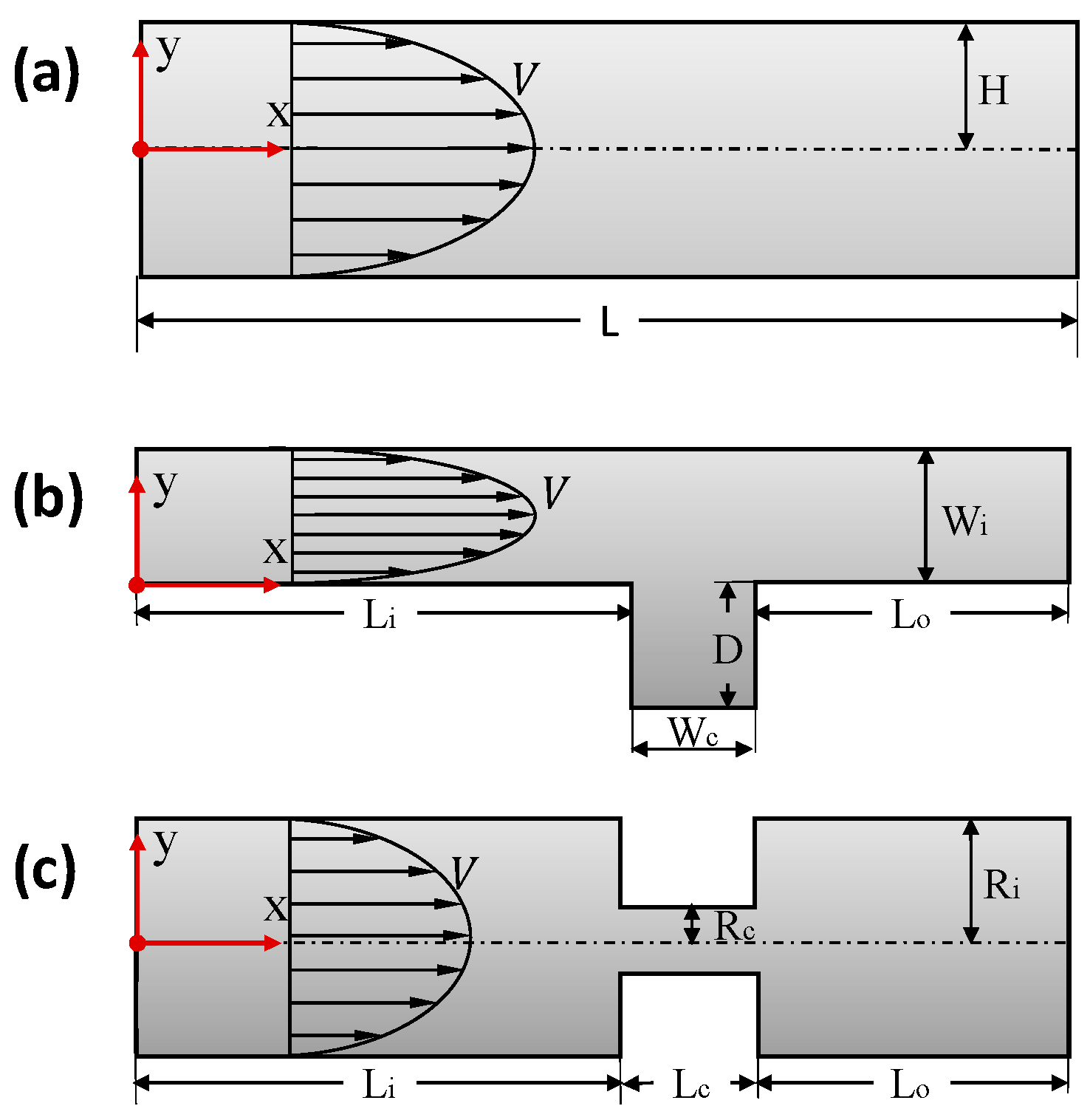
3. Problem Description

In this paper, we assume that the flow is laminar. We investigate the flow of a yield-stress shear-thinning fluid in three different geometries, see Figure 1 for the details. First, we will study the flow in a horizontal and straight channel to reveal the basic features of the fluid, see Figure 1a. Half of the height is H and the length of the channel is kept at 10 H , which is long enough to guarantee that for all the cases the flow near the crevice and the contraction will not be affected by the outlet boundary. The criterion is that the gradient of the dimensionless velocity along the axial direction is less than 10 3 . In order to save computational cost, we have assumed that the flow is two dimensional (axisymmetric).
The second problem is a two-dimensional channel with a crevice representing geometries commonly found in industrial products, such as the parts joints and weld crack, as shown in Figure 1b. The width of the channel is W i and L i is the length of the straight channel, assumed to be 3.3 W i (for a fully developed flow). In order to simulate the effect of crevice, the width W c and the depth D are both set as 0.7 W i . The length of the channel after the crevice is L o = 2 W i .
Figure 1c shows the geometry of a two-dimensional pipe with a contraction, which may represent a portion of a valve in a real industrial application. We also make use of the symmetry in this problem. The radius of the pipe is R i and the radius in the contraction part is R c = 0.3 R i , the length of the contraction is R i , the length of the part before and after the contraction are set as 5 R i and 4 R i , respectively.
Table 1 presented the boundary conditions. The average apparent viscosity is also defined in this paper, η ¯ 1 for the pipe geometry and η ¯ 2 for the channel:
η ¯ 1 = 1 R 2 2 η r d r η ¯ 2 = 1 W η d y .
The grid convergence tests are carried out in order to determine the appropriate meshes to use. Here we only show the results of the straight channel with an inlet generalized Reynolds number of 1 × 10 2 and a Bingham number of 612 ( R e * = 3.3 × 10 3 , B = 15 ) , as shown in Table 2 As a result, Grid C is chosen for further studies. The convergence criterion is that the residuals of pressure and velocity are less than 10 6 and 10 7 , respectively.

4. Results and Discussion

We define a generalized Reynolds number often used in flow of non-Newtonian fluids using the power-law type model [42] ( η = η r γ ˙ n 1 ) :
R e = ρ v 2 n d n η r ( 0.75 + 0.25 n ) n 8 n 1 ,
where d is the inlet diameter. We also use the dimensionless Bingham number B n = τ y H / η r v 0 ( B = ( H / v 0 ) m B n ) to characterize the influence of the yield stress.

4.1. Convergence Properties of the Regularization Methods

For the flow of yield stress fluids, as the yield surface is approached, the presence of the γ ˙ in the denominator of Equation (9) makes the apparent viscosity unbounded. Moreover, while calculating the velocity field, the shape and the location of the yield surface are unknown a priori. To overcome this difficulty, several regularization methods have been proposed; these are continuous and apply to both the yielded and unyielded regions. In this section, we first test the convergence properties of three typical regularization methods, introduced in Section 2.2, on the determination of the yield surface; we do this by simulating the flow of a yield stress fluid in a straight channel for different regularization parameter, ε . We set the reference length and the reference velocity as half of the inlet height and the mean velocity, respectively; we also assume R e = 1.18 × 10 4 , B n = 163   ( R e * = 3.89 × 10 5 , B = 31 ) . The yield surface for different regularization parameter using the three regularization methods are shown in Figure 2 It can be observed that the unyielded region is reduced as ε (the regularization parameter) decreases and eventually converges. In addition, when ε is small enough for convergence, the yield surface of the three regularization methods is nearly at the same position. However, the maximum value of ε required to represent the yield surface is much lower for the Simple model than that of the Papanastasiou and the Bercovier & Engelman models. Therefore, the appropriate choice of the regularization parameter should be made depending on both the flow condition and the regularization method. In the following simulations, the simple regularization method with the proper regularization parameter, ε , is used.

4.2. Flow in a Straight Channel

We first investigate the flow characteristics of a yield-stress, shear-thinning fluid in a straight channel. The reference length and the reference velocity are half of the inlet height and the mean velocity. Typical flow fields with inlet Reynolds number of 1.18 × 10 4 and Bingham number of 612   ( R e * = 3.89 × 10 5 , B = 117 ) are shown in Figure 3 As it can be seen, the maximum value of the velocity is obtained at the center line where the shear rate is almost zero, resulting in a high plastic viscosity. The apparent viscosity depends on both the plastic viscosity and the yield stress, see Equation (9), therefore, the apparent viscosity reaches an extremely high value near the center line. In this region, the fluid has not yielded and it is flowing with the same velocity, as the plug flow. This observation is similar to Abdali’s work (1992) [43] where the flow is fully developed, also see Mitsoulis (2017) [44] for a review of several benchmark problems dealing with yield stress shear-thinning fluids.
Figure 4 shows the velocity and viscosity distributions along the Y-axis for different Reynolds numbers. Here, the reference velocity,   V 0 , is the mean velocity at the inlet, the reference viscosity η r is the viscosity coefficient appearing in the power-law model; the viscosity is plotted in logarithmic coordinates. It can be seen that as the Reynolds number increases, the velocity profile becomes more parabolic and near the axis, the constant-velocity profile becomes smaller, indicating that the size of the unyielded plug is reduced. That is, the shear banding becomes larger. Figure 4b indicates that the plastic viscosity gradually increases near the pipe axis, due to the decreasing of the shear rate; the gradient of the apparent viscosity becomes large near the edge of the plug flow region. The variation of the apparent viscosity is similar to the plastic viscosity; however, with the influence of the yield stress, the magnitude of the apparent viscosity is several times larger than the plastic viscosity. Furthermore, the apparent viscosity in the yield region decreases when the Reynolds number increases, while in the plug flow region, the difference is less significant. The position of high viscosity gradient gradually approaches the center line. The yield region for different Reynolds numbers are shown in Figure 5 It can be seen that the plug flow decreases for larger Reynolds number and the variation is similar to that of the apparent viscosity. The location where the apparent viscosity abruptly changes also roughly coincides with the location where the yield occurs; in addition, due to the flow disturbance the yield surface moves away from the inlet.
In addition, we also consider the effect of the Bingham number. The viscosity and velocity profiles along the Y-axis for different Bingham numbers are plotted in Figure 6. The Bingham number characterizes the ratio of the yield stress to the viscous stress; as the Bingham number increases, the plug size becomes larger. The viscosity increases for higher Bingham numbers, which is in contrast to the behavior for the Reynolds number; furthermore, the maximum value of the apparent viscosity changes with Bingham number. Figure 7 shows the yield region for different Bingham numbers. Similar to the previous studies, the yield region is closely related to the change of the apparent viscosity and the yield surface moves towards the wall and the inlet when the Bingham number increases.
Figure 8 shows the velocity and the viscosity profiles along the Y-axis for different values of m , which indicates the intensity of the shear dependent viscosity. Since in this paper we are assuming that the fluid behaves as a shear-thinning fluid, then the value of m is kept below zero. As observed in Figure 8, the plastic viscosity rises with the increase of the absolute value of m ; on the other hand, the apparent viscosity is negatively proportional to the absolute value of m . Meanwhile, the gradient of the apparent viscosity becomes less as m decreases but the maximum value of the apparent viscosity is hardly affected by m . As the absolute value of m decrease a lower velocity near the pipe center is obtained, resulting in a larger plug flow.

4.3. Flow in a Channel with a Crevice

In this section, we study the flow in a channel with a crevice. The height of the inlet section is chosen as the reference length. Figure 9 shows the velocity fields, streamlines, the shear rate, plastic viscosity and the apparent viscosity distribution when R e = 7.56 × 10 5 and B n = 40.8 ( R e * = 3.89 × 10 5 , B = 7.8 ) . For the flow in the channel with a crevice, the velocity distribution in the main channel is similar to that in the straight channel, where a plug flow is observed near the center of the channel. In the crevice, the velocity and the shear rate remain nearly zero, resulting in a high viscosity and with little or no yielded region. It can also be seen that some of the fluid flows into the crevice; however, it is difficult for the fluid in the deep portion of the crevice to move due to the existence of the yield stress. By looking at the streamlines inside the crevice, we can see that the incoming flow forms a free shear layer near the interface of the main channel and the crevice and the small disturbances grow into vorticial structures that propagate inside the crevice. Furthermore, near the crevice, the flow in the main channel is disturbed a little, resulting in a reduction of the plastic and the apparent viscosity in that region.
The velocity and the viscosity profiles along the line A-A are shown in Figure 10. It can be seen that the velocity is nearly zero in the crevice and near the center of the main channel the velocity has a constant value. In the main channel, the higher Reynolds number leads to higher maximum velocity and smaller plug region, which indicates that the unyielded region can be suppressed by increasing the inlet Reynolds number (usually the inlet velocity); in the crevice, the fluid begins to move as the Reynolds number increases, albeit at low velocity. Along line A-A, the viscosity fluctuates greatly; this could be due to the flow disturbance caused by the presence of the crevice. Interestingly, when the Reynolds number reaches 0.01, the plastic viscosity inside the crevice drops a little and then begins to rise to reach the maximum value, which is in accordance with shape of the vorticial structures observed in the streamlines in the crevice. Figure 11 and Figure 12 show the viscosity profiles in the Y-axis at different X positions, from which we can see that the distribution is no longer consistent with the profiles of the straight channel because of the crevice; the maximum value of the viscosity is no longer in the right of the center of the channel and differs with X positions. The profiles at symmetrical positions along the crevice, such as X = 3.0 and X = 4.3, present similar patterns, see the distributions in Figure 9 and Figure 13. The profiles for the yield region with different Reynolds numbers are shown in Figure 13. It can be seen that the crevice does not play a favorable role for yield stress fluid; as the Reynolds number increases to 0.01, even though more fluid has yielded at the top of the crevice, most of the fluid in the crevice remain stagnant.
Figure 14, Figure 15, Figure 16 and Figure 17 show the effect of the Bingham number. As the Bingham number increases, the velocity decreases, while the viscosity rises, which results in larger unyielded region. In addition, the viscosity becomes more non-linear as the Bingham number increases. The profiles for the yield region are plotted in Figure 17, which has a similar shape to that in Figure 13. Therefore, with higher Reynolds number and lower Bingham number, the size of unyielded plug is reduced.

4.4. Flow in a Pipe with a Contraction

Finally, we consider the flow of a yield stress fluid in a pipe with a contraction. The inlet radius is selected as the reference length. Figure 18 shows the profiles for the velocity, shear rate, plastic viscosity and apparent viscosity when the inlet Reynolds number is 1.18 × 10 4 and B n = 163 ( R e * = 3.89 × 10 5 , B = 31 ) . It is observed that the velocity rises rapidly to several times its value in the contraction, which leads to a higher shear rate and lower viscosity. The shear rate is affected by both the magnitude of the velocity and the shape of the pipe: at the corner M and N where the pipe is suddenly contracted, a minimum shear rate is observed and a higher level of the shear rate is observed at the walls of the contraction and near the two ends of the contracted segment; therefore, the viscosity is higher near the corners and the centerline away from the contraction, forming three unyielded regions in this geometry.
Figure 19 shows the velocity and the viscosity profiles along line B-B for different Reynolds numbers. It can be seen that in the narrow section of the pipe there is a significant increase in the velocity, resulting in smaller plug flow; when the Reynolds number increases, the variation of the velocity profile in the contraction is not as sensitive as that in the regular section of the pipe. The viscosity increases along the radial direction but unlike the straight channel, the maximum value does not occur at the centerline; the viscosity also decreases after reaching a maximum, which indicates that the effect of the inlet and outlet of the contraction. To investigate this effect, the viscosity profiles along the radial direction at different X positions are plotted in Figure 20 and Figure 21. It can be seen that the maximum apparent viscosity appears at the position near the center line away from the contraction and the stagnant zones at the corners. A change in the geometry would change the streamlines and lead to a higher shear rate, as a result, the viscosity decreases upstream and downstream of the contraction. Furthermore, for a yield-stress fluid, the high Reynolds number can help the fluid approach a lower viscosity.
From the yield regions shown in Figure 22, which is strongly related to the viscosity, we can see that the unyielded regions are roughly symmetric with respect to the contraction. The size of the plug flow continues to reduce while the Reynolds number keeps increasing.
The effect of the Bingham number is shown in Figure 23, Figure 24, Figure 25 and Figure 26 With smaller Bingham numbers, it is easier for the fluid to flow; this results in a lower apparent viscosity and a more parabolic velocity profile. And as the Bingham number approaches smaller values, the unyielded region is observed only near the corners. Alexandrou et al. (2001) [45] showed similar results in the entry-expansion flow, where the geometry studied in their work is similar to the third case in our study. When designing a transport system, for example, a proper Bingham number (flow condition) should be considered in order to achieve an acceptable maximum unyielded region which is considered unfavorable in engineering applications. Furthermore, as the Reynolds number increases, the flow may become unstable after the channel contraction; this has been observed for the Casson, the Power-Law and the Quemada fluid models. The instability behavior depends on the specific parameters involved in each model’s constitutive equation [46].

5. Conclusions

In this paper, we have numerically studied the flow of dense suspension exhibiting yield-stress and shear-thinning effects. The rheological characteristics of such complex fluids need to be understood in engineering process. The dense suspension is modeled as a Herschel-Bulkley fluid and three benchmark geometries are investigated: a straight channel, a channel with a crevice and a pipe with a contraction. According to the numerical simulations, the following conclusions can be drawn:
  • Three representative regularization methods are used to look at the convergence properties on the determination of the yield surface; these methods are (1) the Simple model; (2) the Papanastasiou model and (3) the Bercovier and Engelman model. The yield surface could be described reasonably with a proper choice of the regularization parameter, ε , depending on the regularization method and the flow conditions. However, the maximum value of ε required to represent the yield surface is much lower for the Simple model than for the Papanastasiou and the Bercovier and Engelman models.
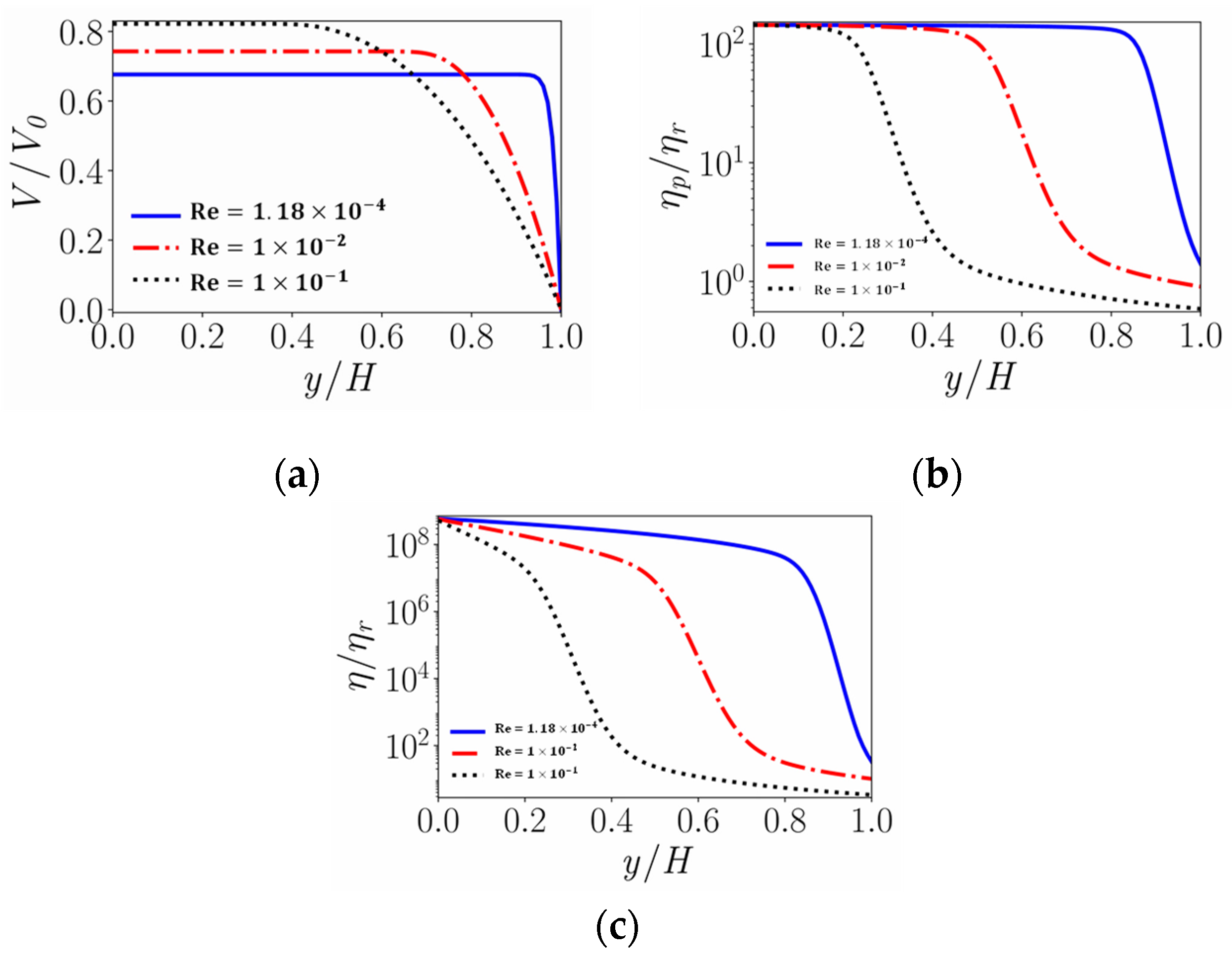
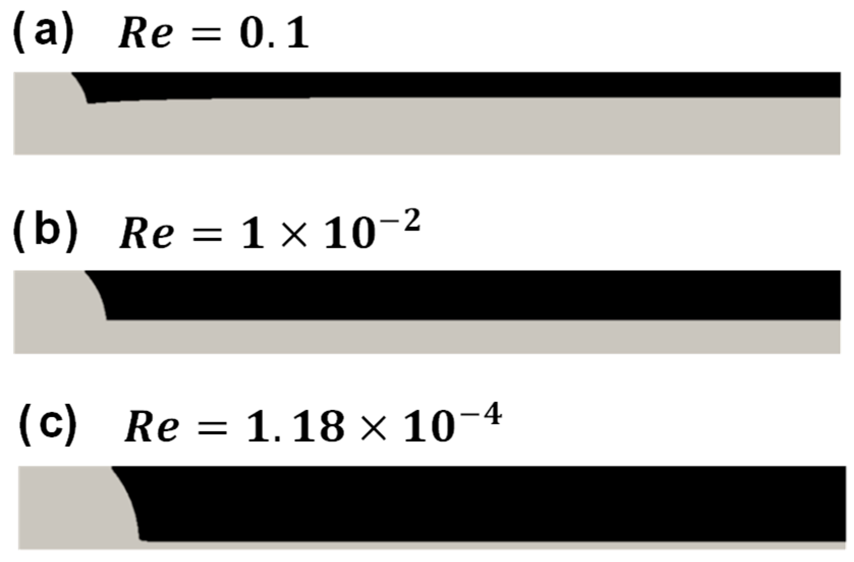
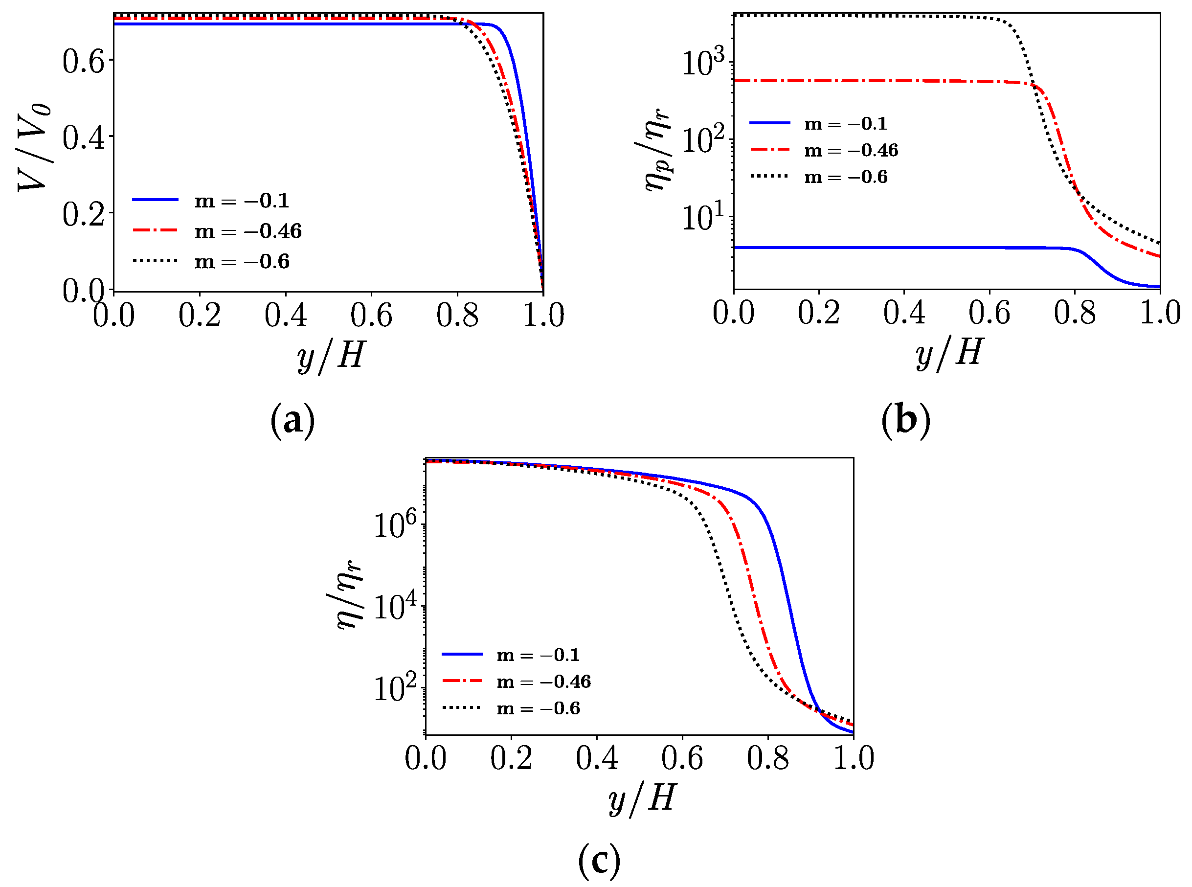
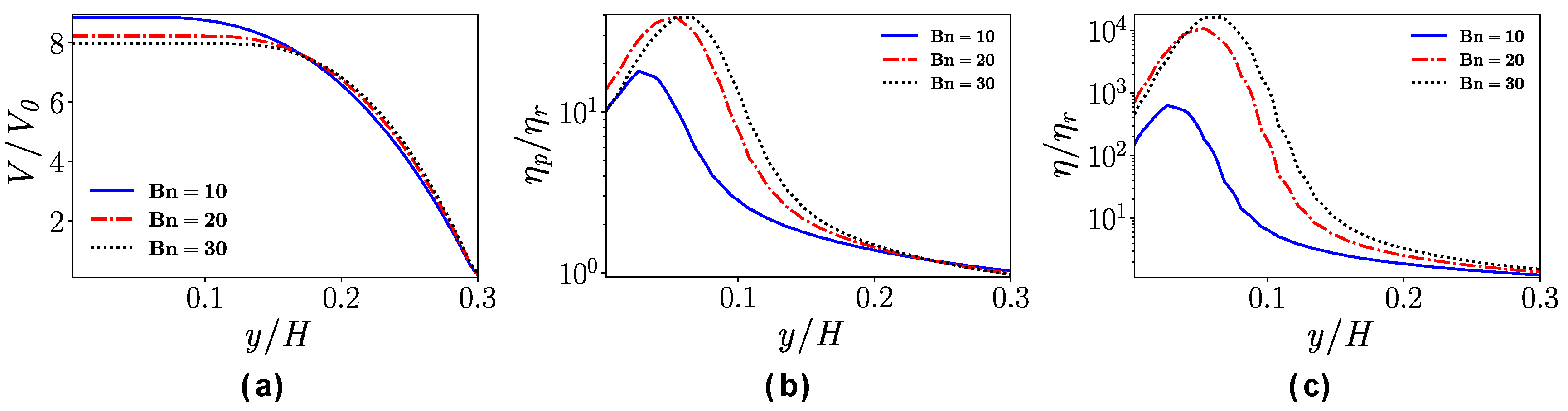
  • In the straight channel, for flows with low Reynolds number and high Bingham number, a plug region near the center line where the stress is below the yield stress will form. For shear-thinning fluids, the viscosity parameter n has a similar influence on the velocity profiles as the Bingham number.
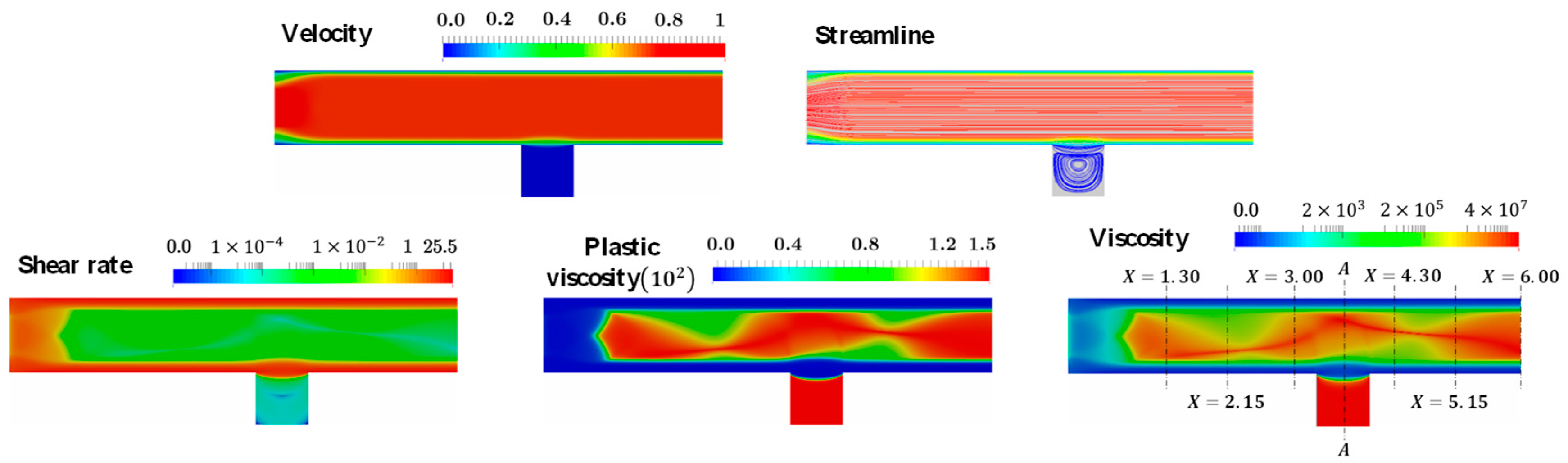
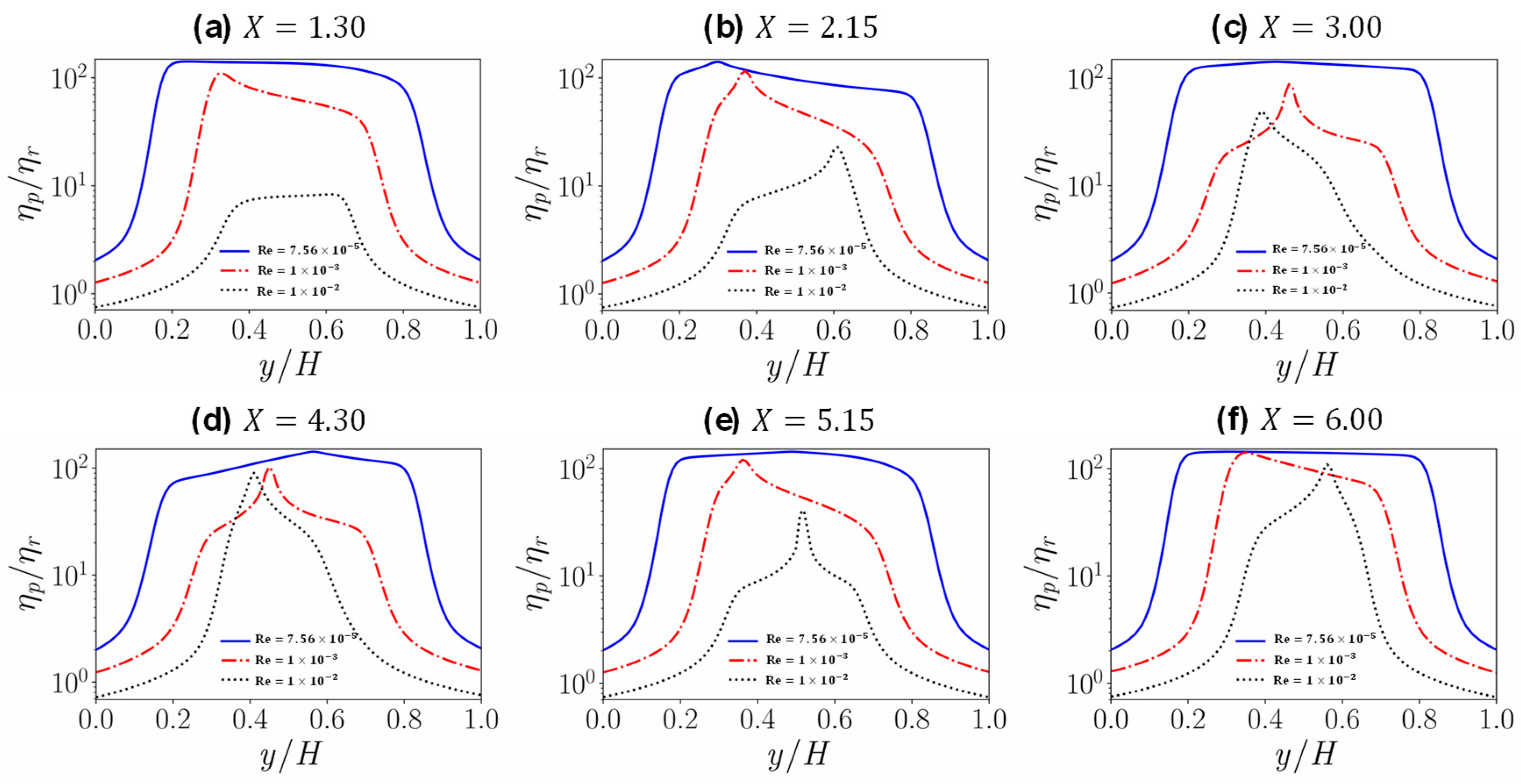
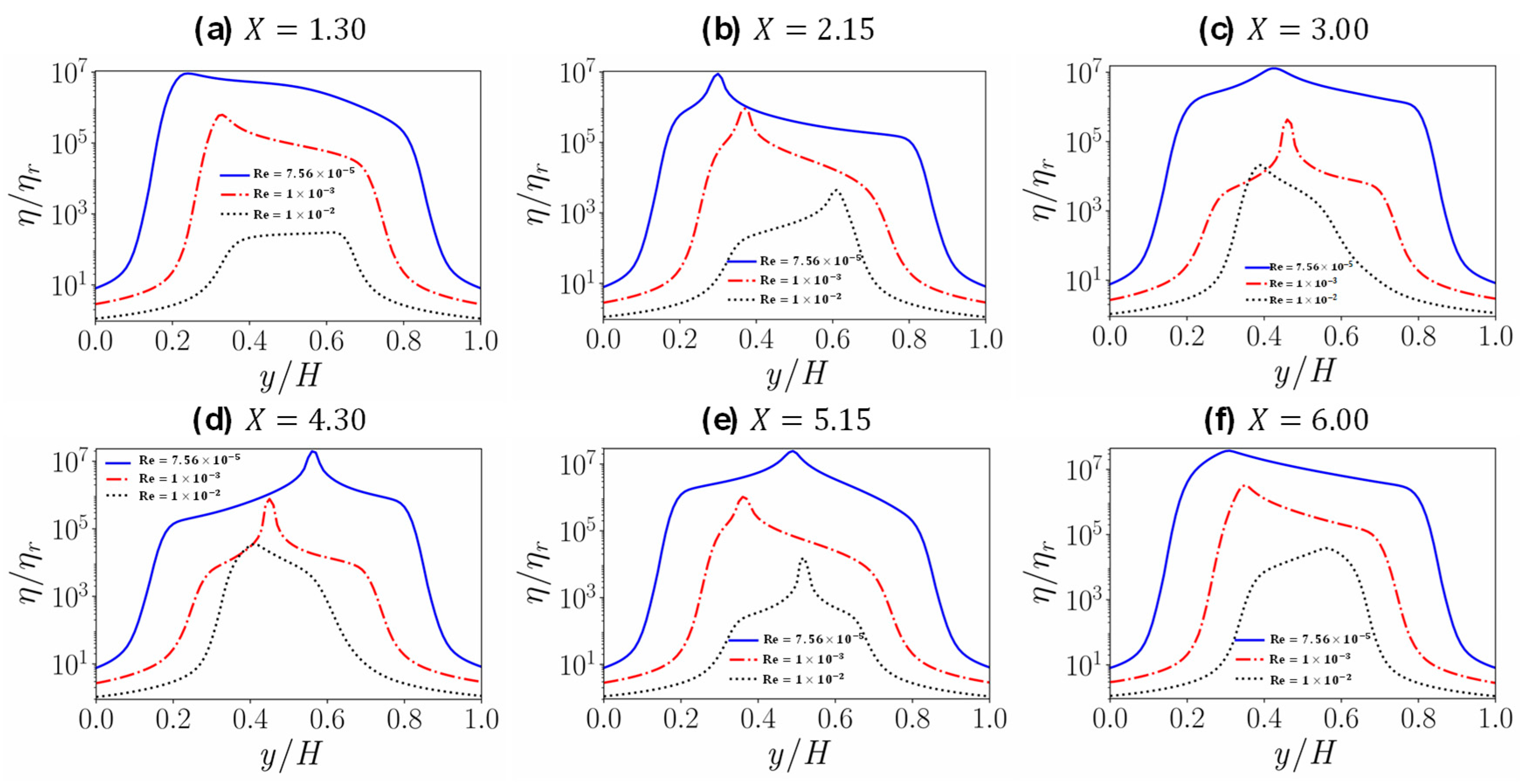
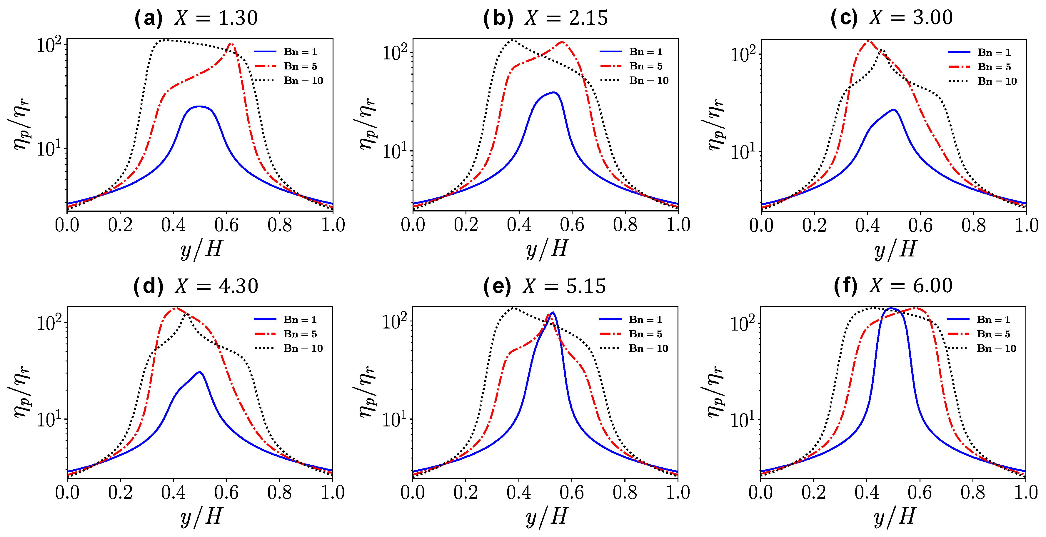
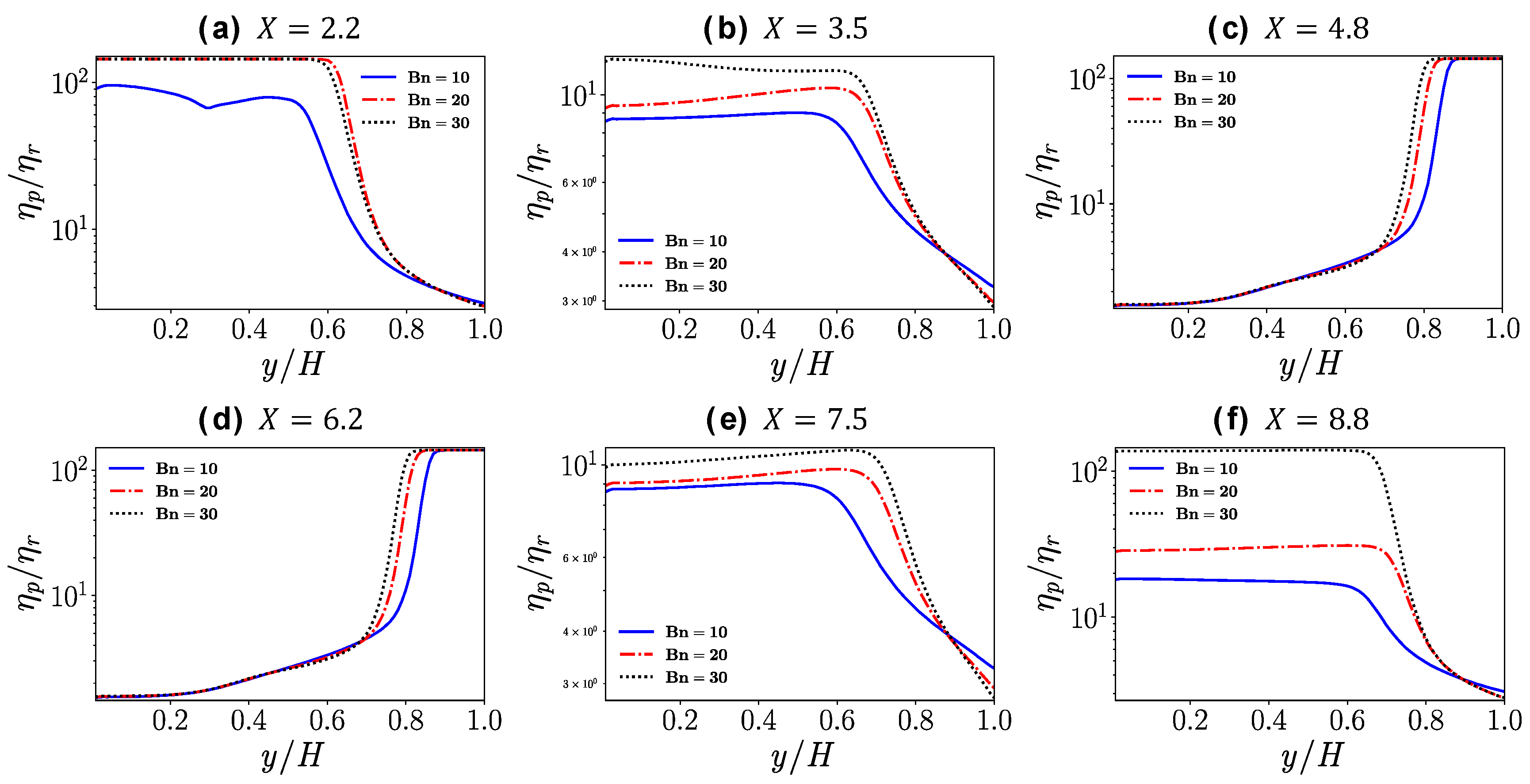
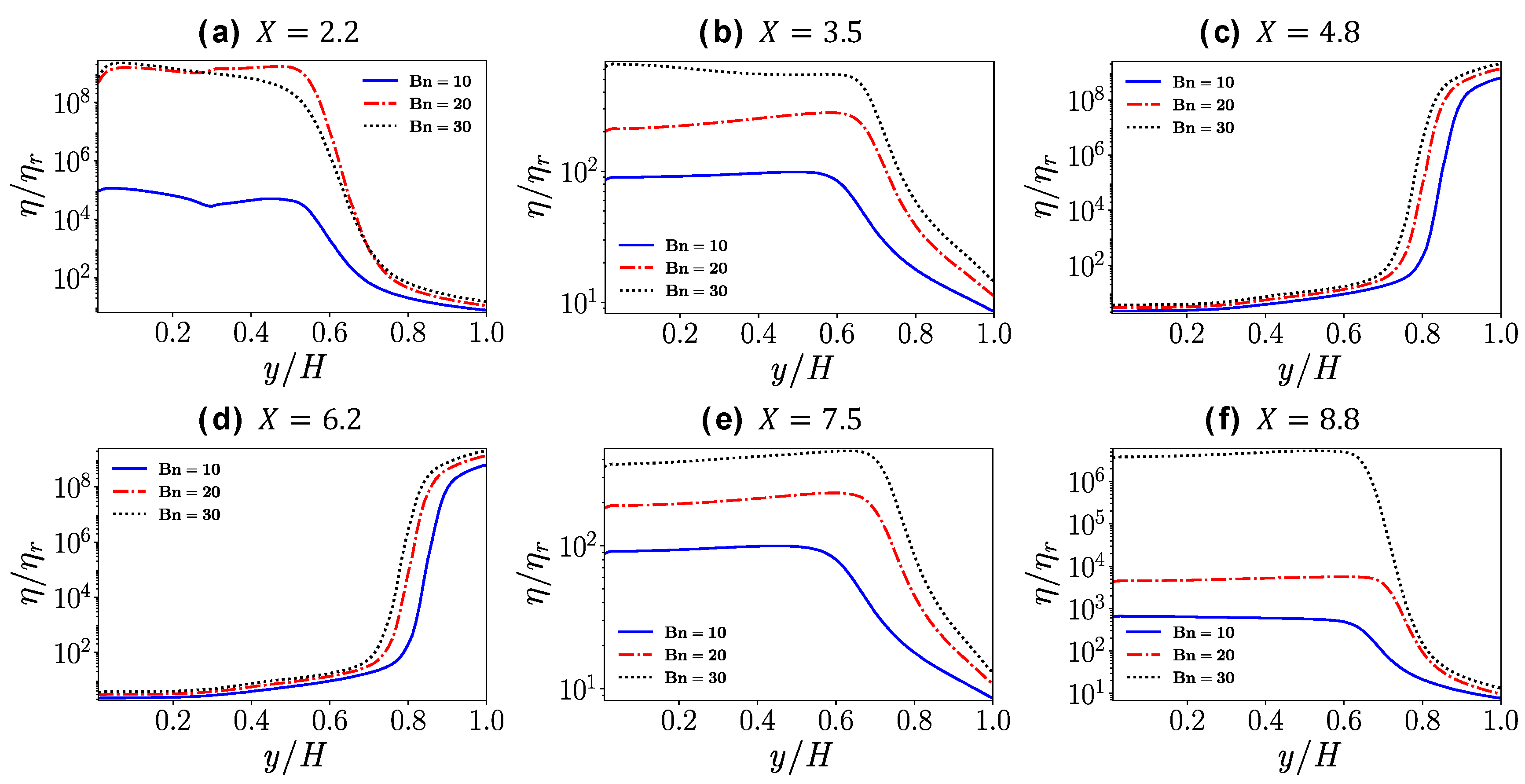
  • In the case of the channel with a crevice, even though some vorticial structures seem to propagate inside the crevice due to the free shear layer near the interface of the main channel and the crevice, the fluid in the deeper portion of the crevice still has high apparent viscosity because of the existence of the yield stress, forming an unyielded region. Furthermore, near the crevice the flow near the interface of the main channel and the crevice is disturbed a little; this results in a reduction of the plastic viscosity and the apparent viscosity.
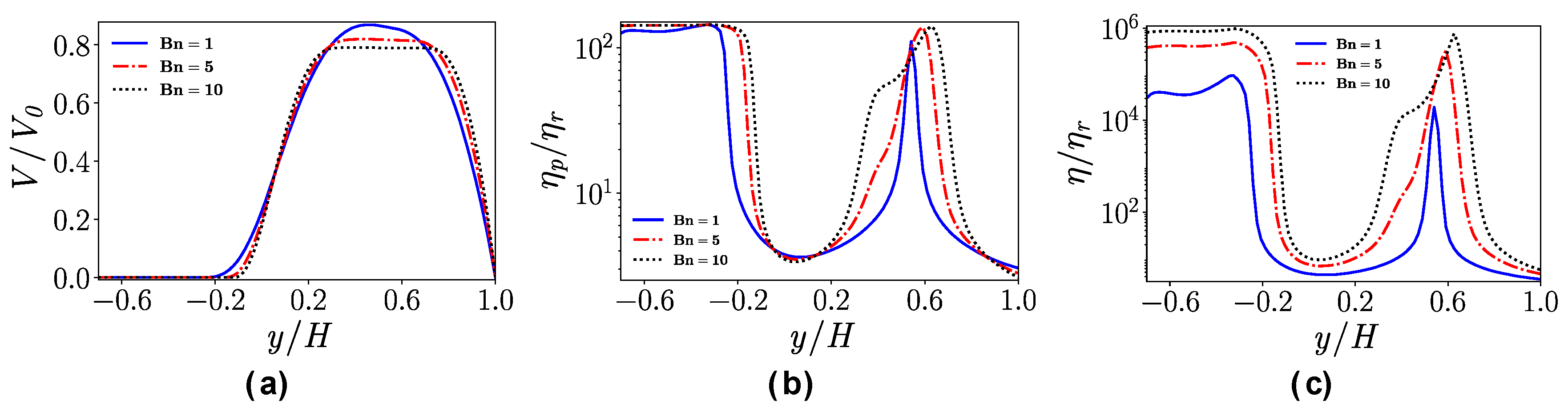
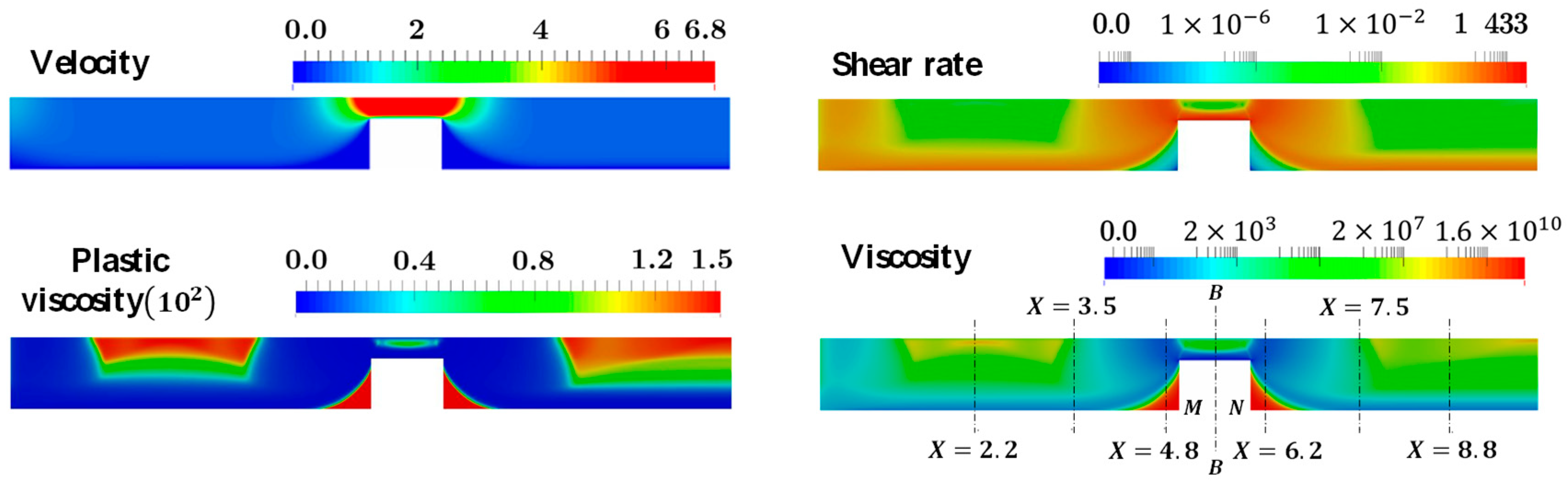
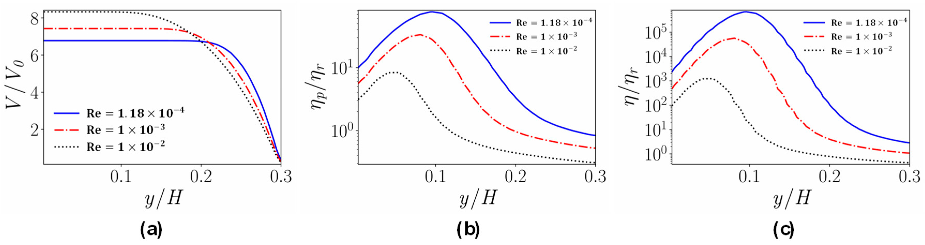
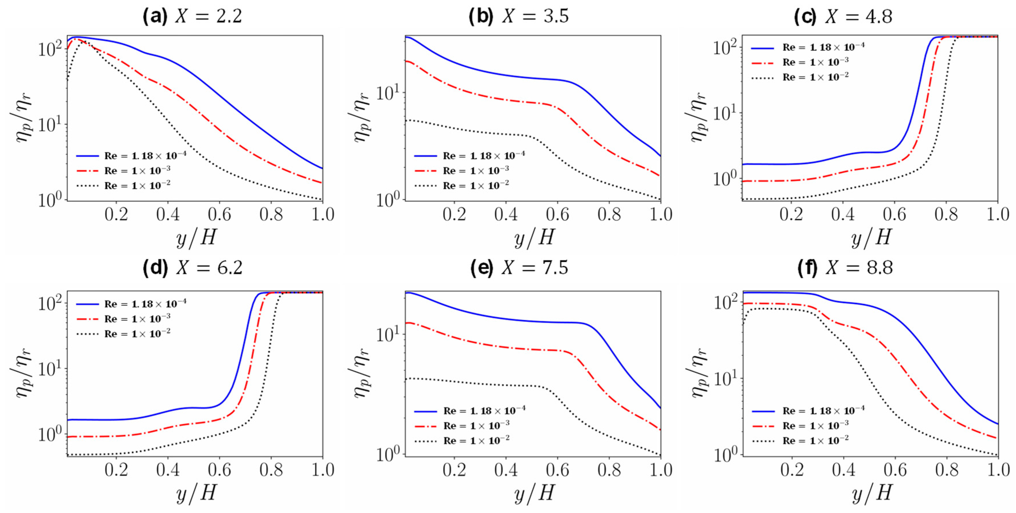
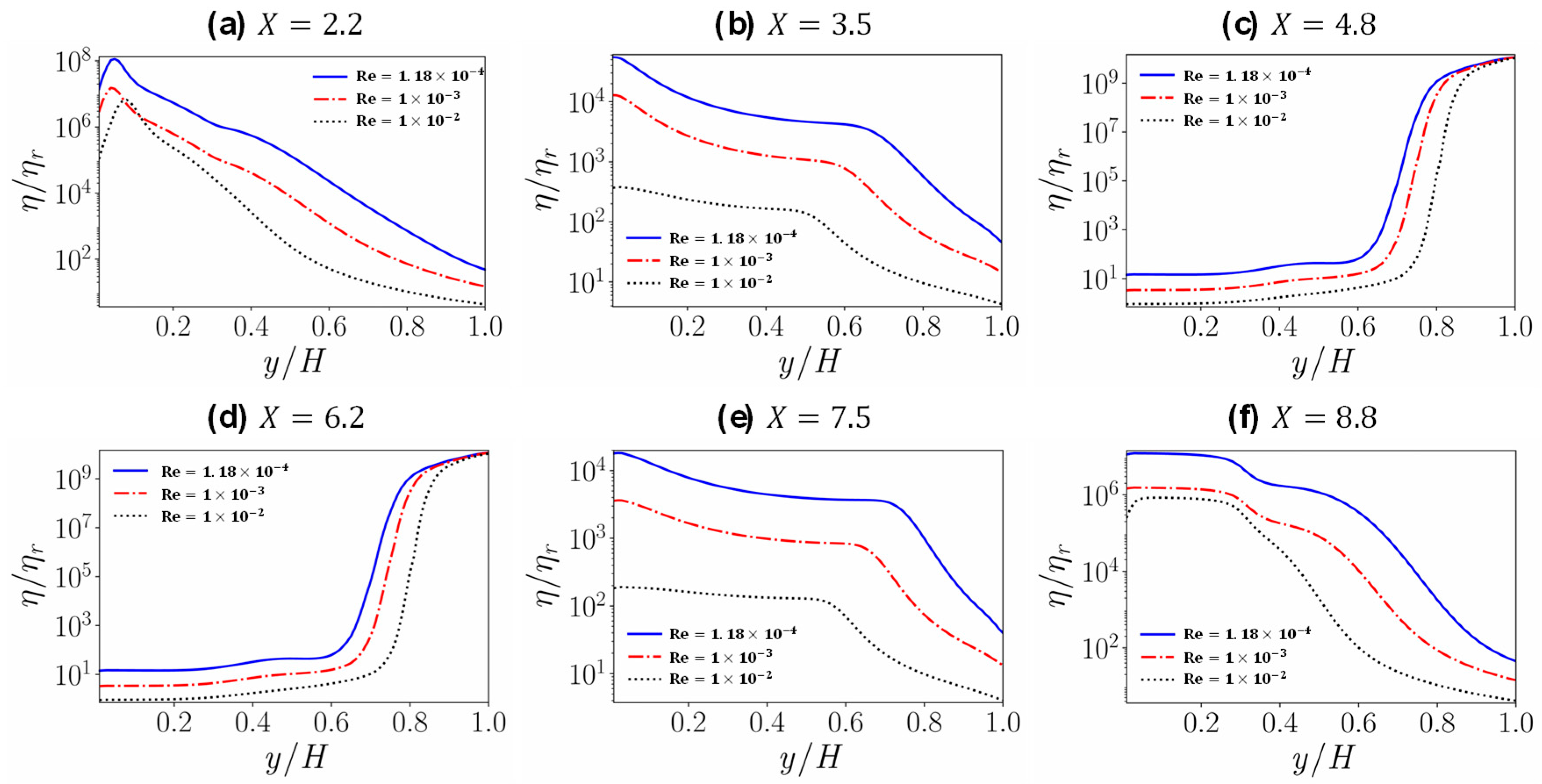
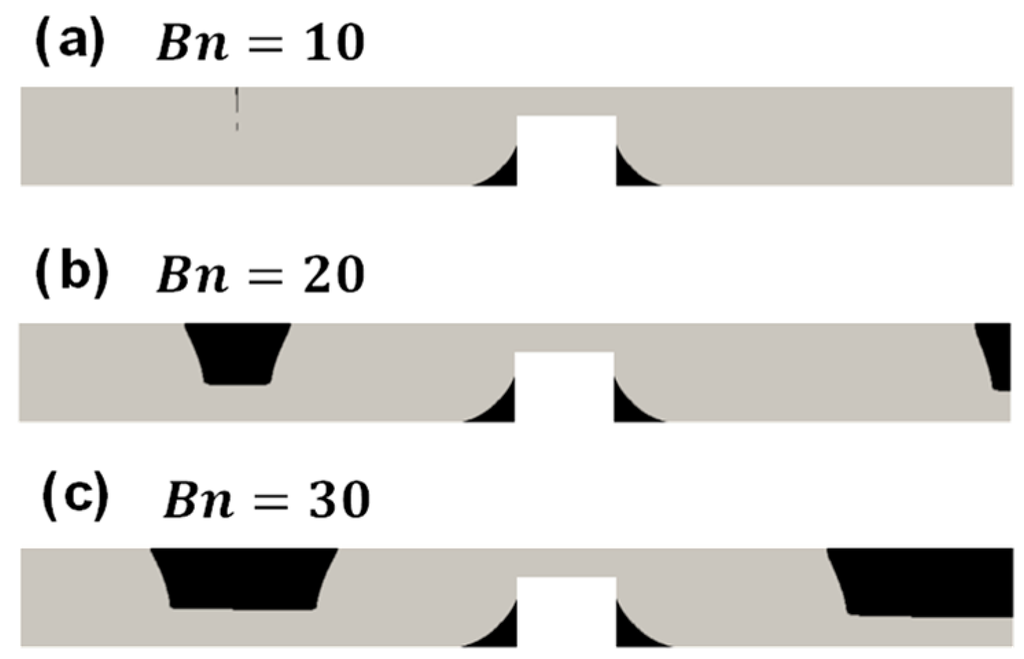
  • For the pipe with a contraction, near the neck, the unyielded region reduces significantly due to the enhanced flow disturbance; while the shear rate is nearly zero at the bottom corner of the contraction segment, resulting in a very small yielded region.
  • For the Bingham numbers considered in this work, further increasing the Reynolds number leads to the disappearance of the yield region. The yield phenomenon can still be observed if both the Reynolds number and the Bingham number are increased; this is an important issue and a problem more demanding in computational time; we plan to study this in the near future.

Author Contributions

M.-G.L. developed the framework of the paper and did the numerical simulations. M.M. and W.-T.W. derived the equations. M.-G.L., M.M., F.F. and W.-T.W. prepared the manuscript. All authors have read and agreed to the published version of the manuscript.

Funding

This research was funded by Natural Science Foundation of China, grant number 11802135 and the Fundamental Research Funds for the Central Universities, grant number 30919011401.

Conflicts of Interest

The authors declare no conflict of interest. The funders had no role in the design of the study; in the collection, analyses, or interpretation of data; in the writing of the manuscript, or in the decision to publish the results.

Nomenclature

bbody force vector (N)
B ratio of the yield stress to the viscous stress
B n Bingham number
A 1 Related to the symmetric part of velocity gradient ( 1 / s )
d i v divergence operator
g r a d gradient operator
Hreference length ( m )
m material parameter ( m = n 1 )
n material parameter
p pressure (Pa)
R e * Generalized Reynolds number
R e generalized Reynolds number
t time
T stress tensor (Pa)
T y yield stress (Pa)
T v viscous stress (Pa)
v velocity vector (m/s)
V dimensionless velocity vector
X , Y dimensionless Cartesian coordinates
x position vector (m)
X dimensionless position vector
Greek symbols
ρ density of fluid (kg/m3)
η dynamic viscosity (Pa∙s)
η p plastic viscosity (Pa∙s)
ε regularization parameter
γ ˙ shear rate ( 1 / s )
τ dimensionless time
τ y yield stress (Pa)

References

  1. Ferry, J.D.; Ferry, J.D. Viscoelastic Properties of Polymers; John Wiley & Sons: Hoboken, NJ, USA, 1980. [Google Scholar]
  2. Natan, B.; Rahimi, S. The status of gel propellants in year 2000. Int. J. Energ. Mater. Chem. Propuls. 2009, 5, 172–194. [Google Scholar] [CrossRef]
  3. Bonn, D.; Denn, M.M. Yield stress fluids slowly yield to analysis. Science 2009, 324, 1401–1402. [Google Scholar] [CrossRef] [PubMed]
  4. Putz, A.M.V.; Burghelea, T.I. The solid–fluid transition in a yield stress shear thinning physical gel. Rheol. Acta 2009, 48, 673–689. [Google Scholar] [CrossRef] [Green Version]
  5. Barnes, H.A. Thixotropy—A review. J. Nonnewton. Fluid Mech. 1999, 81, 133–178. [Google Scholar] [CrossRef]
  6. Stickel, J.J.; Powell, R.L. Fluid mechanics and rheology of dense suspensions. Annu. Rev. Fluid Mech. 2005, 37, 129–149. [Google Scholar] [CrossRef]
  7. Barnes, H.A.; Walters, K. The yield stress myth? Rheol. Acta 1985, 24, 323–326. [Google Scholar] [CrossRef]
  8. Coussot, P.; Nguyen, Q.D.; Huynh, H.T.; Bonn, D. Avalanche behavior in yield stress fluids. Phys. Rev. Lett. 2002, 88, 175501. [Google Scholar] [CrossRef] [PubMed] [Green Version]
  9. Zhu, L.; De Kee, D. Slotted-plate device to measure the yield stress of suspensions: Finite element analysis. Ind. Eng. Chem. Res. 2002, 41, 6375–6382. [Google Scholar] [CrossRef]
  10. Qian, Y.; Kawashima, S. Distinguishing dynamic and static yield stress of fresh cement mortars through thixotropy. Cem. Concr. Compos. 2018, 86, 288–296. [Google Scholar] [CrossRef]
  11. Malkin, A.; Kulichikhin, V.; Ilyin, S. A modern look on yield stress fluids. Rheol. Acta 2017, 56, 177–188. [Google Scholar] [CrossRef]
  12. Coussot, P. Yield stress fluid flows: A review of experimental data. J. Nonnewton. Fluid Mech. 2014, 211, 31–49. [Google Scholar] [CrossRef]
  13. Gomes, A.F.C.; Marinho, J.L.G.; Santos, J.P.L. Numerical simulation of drilling fluid behavior in different depths of an oil well. Braz. J. Pet. Gas 2019, 13, 309–322. [Google Scholar] [CrossRef]
  14. Saeid, N.H.; Busahmin, B.S. Numerical investigations of drilling mud flow characteristics in vertical well. An Int. J. (ESTIJ) 2017, 6, 2250–3498. [Google Scholar]
  15. Subramanian, R.; Azar, J.J. Experimental study on friction pressure drop for nonnewtonian drilling fluids in pipe and annular flow. Soc. Pet. Eng. Int. Oil Gas Conf. Exhib. China 2000 IOGCEC 2000 2000. [Google Scholar] [CrossRef]
  16. Ovarlez, G.; Mahaut, F.; Deboeuf, S.; Lenoir, N.; Hormozi, S.; Chateau, X. Flows of suspensions of particles in yield stress fluids. J. Rheol. 2015, 59, 1449–1486. [Google Scholar] [CrossRef] [Green Version]
  17. Saasen, A.; Ytrehus, J.D. Viscosity models for drilling fluids—Herschel-bulkley parameters and their use. Energies 2020, 13, 5271. [Google Scholar] [CrossRef]
  18. Soo, S.L. Multiphase Fluid Dynamics; Science Press: Beijing, China, 1990. [Google Scholar]
  19. Rajagopal, K.R.; Tao, L. Mechanics of Mixtures; World Scientific: Singapore, 1995; Volume 35. [Google Scholar]
  20. Johnson, G.; Massoudi, M.; Rajagopal, K.R. Flow of a fluid infused with solid particles through a pipe. Int. J. Eng. Sci. 1991, 29, 649–661. [Google Scholar] [CrossRef]
  21. Massoudi, M. A mixture theory formulation for hydraulic or pneumatic transport of solid particles. Int. J. Eng. Sci. 2010, 48, 1440–1461. [Google Scholar] [CrossRef]
  22. Phillips, R.J.; Armstrong, R.C.; Brown, R.A.; Graham, A.L.; Abbott, J.R. A constitutive equation for concentrated suspensions that accounts for shear-induced particle migration. Phys. Fluids A 1992, 4, 30–40. [Google Scholar] [CrossRef]
  23. Zhou, Z.; Wu, W.-T.; Massoudi, M. Fully developed flow of a drilling fluid between two rotating cylinders. Appl. Math. Comput. 2016, 281, 266–277. [Google Scholar] [CrossRef]
  24. Tao, C.; Kutchko, B.G.; Rosenbaum, E.; Wu, W.T.; Massoudi, M. Steady flow of a cement slurry. Energies 2019, 12, 2604. [Google Scholar] [CrossRef] [Green Version]
  25. Peker, S.M.; Helvaci, S.S. Solid-liquid Two Phase Flow; Elsevier: Amsterdam, The Netherlands, 2011. [Google Scholar]
  26. Slattery, J.C. Advanced Transport Phenomena; Cambridge University Press: Cambridge, UK, 1999. [Google Scholar]
  27. Li, Y.; Wu, W.-T.; Liu, X.; Massoudi, M. The effects of particle concentration and various fluxes on the flow of a fluid-solid suspension. Appl. Math. Comput. 2019, 358, 151–160. [Google Scholar] [CrossRef]
  28. Massoudi, M.; Vaidya, A. On some generalizations of the second grade fluid model. Nonlinear Anal. Real World Appl. 2008, 9, 1169–1183. [Google Scholar] [CrossRef]
  29. Roscoe, R. Suspensions, flow properties of disperse systems. In Flow Properties of Disperse Systems; Hermans, J.J., Ed.; North Holland Publishing Company: Amsterdam, The Netherlands, 1953. [Google Scholar]
  30. Tabuteau, H.; Coussot, P.; de Bruyn, J.R. Drag force on a sphere in steady motion through a yield-stress fluid. J. Rheol. 2007, 51, 125–137. [Google Scholar] [CrossRef]
  31. Coussot, P.; Tocquer, L.; Lanos, C.; Ovarlez, G. Macroscopic vs. local rheology of yield stress fluids. J. NonNewton Fluid Mech. 2009, 158, 85–90. [Google Scholar] [CrossRef]
  32. Cao, Q.-L.; Massoudi, M.; Liao, W.-H.; Feng, F.; Wu, W.-T. Flow characteristics of water-HPC gel in converging tubes and tapered injectors. Energies 2019, 12, 1643. [Google Scholar] [CrossRef] [Green Version]
  33. Mas, R.; Magnin, A. Experimental validation of steady shear and dynamic viscosity relation for yield stress fluids. Rheol. Acta 1997, 36, 49–55. [Google Scholar] [CrossRef]
  34. Denn, M.M.; Bonn, D. Issues in the flow of yield-stress liquids. Rheol. Acta 2011, 50, 307–315. [Google Scholar] [CrossRef] [Green Version]
  35. White, J.L. A plastic-viscoelastic constitutive equation to represent the rheological behavior of concentrated suspensions of small particles in polymer melts. J. NonNewton Fluid Mech. 1979, 5, 177–190. [Google Scholar] [CrossRef]
  36. Prager, W. Introduction to Mechanics of Continua; Courier Corporation: North Chelmsford, MA, USA, 2004. [Google Scholar]
  37. Putz, A.; Frigaard, I.A.; Martinez, D.M. On the lubrication paradox and the use of regularisation methods for lubrication flows. J. NonNewton Fluid Mech. 2009, 163, 62–77. [Google Scholar] [CrossRef]
  38. Frigaard, I.A.; Nouar, C. On the usage of viscosity regularisation methods for visco-plastic fluid flow computation. J. NonNewton Fluid Mech. 2005, 127, 1–26. [Google Scholar] [CrossRef]
  39. Allouche, M.; Frigaard, I.A.; Sona, G. Static wall layers in the displacement of two visco-plastic fluids in a plane channel. J. Fluid Mech. 2000, 424, 243–277. [Google Scholar] [CrossRef]
  40. Bercovier, M.; Engelman, M. A finite-element method for incompressible non-Newtonian flows. J. Comput. Phys. 1980, 36, 313–326. [Google Scholar] [CrossRef]
  41. Papanastasiou, T.C. Flows of materials with yield. J. Rheol. 1987, 31, 385–404. [Google Scholar] [CrossRef]
  42. Von Kampen, J.; Madlener, K.; Ciezki, H.K. Characteristic flow and spray properties of gelled fuels with regard to the impinging jet injector type. In Proceedings of the 42nd AIAA Joint Propulsion Conference, Sacramento, California, USA, 9–12 July 2006; Volume 4, pp. 2639–2650. [Google Scholar]
  43. Abdali, S.S.; Mitsoulis, E.; Markatos, N.C. Entry and exit flows of Bingham fluids. J. Rheol. 1992, 36, 389–407. [Google Scholar] [CrossRef]
  44. Mitsoulis, E.; Tsamopoulos, J. Numerical simulations of complex yield-stress fluid flows. Rheol. Acta 2017, 56, 231–258. [Google Scholar] [CrossRef]
  45. Alexandrou, A.N.; McGilvreay, T.M.; Burgos, G. Steady herschel-bulkley fluid flow in three-dimensional expansions. J. NonNewton Fluid Mech. 2001, 100, 77–96. [Google Scholar] [CrossRef]
  46. Neofytou, P.; Drikakis, D. Non-Newtonian flow instability in a channel with a sudden expansion. J. NonNewton Fluid Mech. 2003, 111, 127–150. [Google Scholar] [CrossRef]
Figure 1. Schematic of (a) straight channel (b) channel with a crevice (c) pipe with a contraction.
Energies 13 06635 g001
Figure 2. Yield surfaces in the straight channel with different regularization parameter using: (a) Simple; (b) Papanastasiou; (c) Bercovier & Engelman models.
Energies 13 06635 g002
Figure 3. Velocity, shear rate, plastic viscosity and apparent viscosity fields in a straight channel with inlet Reynolds number of 1.18 × 10 4 and B n = 612 .
Energies 13 06635 g003
Figure 4. Profiles for: (a) velocity; (b) plastic viscosity; (c) apparent viscosity along the Y-axis in the straight channel for different inlet Reynolds numbers.
Energies 13 06635 g004
Figure 5. Distribution of the yield surfaces for different Reynolds numbers. The shaded regions are unyielded.
Energies 13 06635 g005
Figure 6. Profiles for: (a) velocity; (b) plastic viscosity; (c) the apparent viscosity along the Y-axis in the straight channel for different Bingham numbers and R e = 1.18 × 10 4 .
Energies 13 06635 g006
Figure 7. Distribution of the yield surfaces for different Bingham numbers and R e = 1.18 × 10 4 . The shaded regions are unyielded.
Energies 13 06635 g007
Figure 8. Profiles for: (a) velocity; (b) plastic viscosity; (c) apparent viscosity along the Y-axis in the straight channel for different values of the exponent m in the power law model.
Energies 13 06635 g008
Figure 9. The velocity, streamlines, shear rate, plastic viscosity and plastic viscosity fields in the channel with a crevice with an inlet Reynolds number of 7.56 × 10 5 and B n = 40.8 .
Energies 13 06635 g009
Figure 10. (a) Velocity; (b) Plastic viscosity; (c) Apparent viscosity profiles along line A-A for different inlet Reynolds numbers.
Energies 13 06635 g010
Figure 11. Plastic viscosity profiles along the Y-axis at different X positions for different Reynolds numbers ( X = x / H ).
Energies 13 06635 g011
Figure 12. Apparent viscosity profiles along the Y-axis at different X positions for different Reynolds numbers ( X = x / H ).
Energies 13 06635 g012
Figure 13. Distribution of the yield surfaces for different Reynolds numbers. The shaded regions are unyielded.
Energies 13 06635 g013
Figure 14. (a) Velocity (b) Plastic viscosity (c) Apparent viscosity profiles along A-A for different Bingham numbers and R e = 7.56 × 10 5 .
Energies 13 06635 g014
Figure 15. Plastic viscosity profiles along the Y-axis at different X positions for different Bingham numbers ( X = x / H ).
Energies 13 06635 g015
Figure 16. Apparent viscosity profiles along the Y-axis at different X positions for different Bingham numbers ( X = x / H ).
Energies 13 06635 g016
Figure 17. Distribution of the yield surfaces for different Bingham numbers and R e = 7.56 × 10 5 . The shaded regions are unyielded.
Energies 13 06635 g017
Figure 18. Velocity, shear rate, plastic viscosity and apparent viscosity fields in the pipe with a contraction when the inlet Reynolds number is 1.18 × 10 4 and B n = 163 .
Energies 13 06635 g018
Figure 19. (a) Velocity; (b) Plastic viscosity; (c) Apparent viscosity profiles along line B-B for different Reynolds numbers.
Energies 13 06635 g019
Figure 20. Plastic viscosity profiles along the radial direction at different X positions for different Reynolds numbers ( X = x / H ).
Energies 13 06635 g020
Figure 21. Apparent viscosity profiles along the radial direction at different X positions for different Reynolds numbers ( X = x / H ).
Energies 13 06635 g021
Figure 22. Distribution of the yield surfaces for different Reynolds numbers. The shaded regions are unyielded.
Energies 13 06635 g022
Figure 23. (a) Velocity (b) Plastic viscosity (c) Apparent viscosity profiles along B-B for different Bingham numbers and R e = 1.18 × 10 4 .
Energies 13 06635 g023
Figure 24. Plastic viscosity profiles along the radial direction at different X positions for different Bingham numbers and R e = 1.18 × 10 4 ( X = x / H ).
Energies 13 06635 g024
Figure 25. Apparent viscosity profiles along the radial direction at different X positions for different Bingham numbers and R e = 1.18 × 10 4 ( X = x / H ).
Energies 13 06635 g025
Figure 26. Distribution of the yield surfaces for different Bingham numbers with R e = 1.18 × 10 4 . The shaded regions are unyielded.
Energies 13 06635 g026
Table 1. Boundary conditions used in the numerical simulations.
Boundary TypeBoundary Conditions
PressureVelocity
WallZero gradientFixed value (0)
InletZero gradientFixed value
OutletFixed value (0)Zero gradient
Table 2. Mesh dependency study.
LabelGrid NumberMean Plastic Viscosity at Exit (102)
Grid A25,0002.12074
Grid B43,9562.04562
Grid C69,1042.00631
Grid D100,0001.99802
Publisher’s Note: MDPI stays neutral with regard to jurisdictional claims in published maps and institutional affiliations.

