Article

A Methodology for Long-Term Model Predictive Control of Hybrid Geothermal Systems: The Shadow-Cost Formulation

by
Iago Cupeiro Figueroa
1,2,*,
Massimo Cimmino
3,* and
Lieve Helsen
1,2
1
Department of Mechanical Engineering, University of Leuven (KU Leuven), 3001 Leuven, Belgium
2
EnergyVille, Thor Park 8310, 3600 Genk, Belgium
3
École Polytechnique de Montréal, Département de Génie Mécanique, Université de Montréal, Montréal, QC H3C3A7, Canada
*
Authors to whom correspondence should be addressed.
Energies 2020, 13(23), 6203; https://doi.org/10.3390/en13236203
Submission received: 20 October 2020 / Revised: 20 November 2020 / Accepted: 23 November 2020 / Published: 25 November 2020
(This article belongs to the Special Issue Advances in Ground Heat Exchangers and Ground-Coupled Heat Pumps)

Abstract

:
Model Predictive Control (MPC) predictive’s nature makes it attractive for controlling high-capacity structures such as thermally activated building systems (TABS). Using weather predictions in the order of days, the system is able to react in advance to changes in the building heating and cooling needs. However, this prediction horizon window may be sub-optimal when hybrid geothermal systems are used, since the ground dynamics are in the order of months and even years. This paper proposes a methodology that includes a shadow-cost in the objective function to take into account the long-term effects that appear in the borefield. The shadow-cost is computed for a given long-term horizon that is discretized over time using predictions of the building heating and cooling needs. The methodology is applied to a case with only heating and active regeneration of the ground thermal balance. Results show that the formulation with the shadow cost is able to optimally use the active regeneration, reducing the overall operational costs at the expenses of an increased computational time. The effects of the shadow cost long-term horizon and the predictions accuracy are also investigated.

1. Introduction

Model Predictive Control (MPC) is an optimal control methodology that has shown a significant potential for energy and cost savings in building energy systems operation. In some real pilot buildings where it has been implemented, it has achieved savings between 15 and 30% [1,2,3]. The MPC principle is based on using a model of the system and disturbances predictions to forecast its future behavior over a prediction horizon. Using this information, an optimization problem is solved to find the optimal control sequence that minimizes a given cost or objective function under a specific set of constraints. MPC relies on a ‘receding horizon’ strategy, i.e., at each control time-step only the first control signal of the sequence is applied and the prediction horizon is shifted towards the future step, where the optimization problem is solved again. The concept of MPC is not new, since it originated in the chemical and automotive industries in the late 70s [4], but only over the last decade it has been more extensively researched within the building sector. Applied to buildings, MPC uses a model of the building envelope and energy system along with weather and occupancy forecasts to predict the building dynamic behavior and the energy system efficiencies. Typical objective functions in buildings include energy use, costs and CO 2 emissions which can have variable prices and emission factors over time [5]. The objective is minimized while satisfying thermal comfort, humidity and air quality constraints.
MPC is especially interesting in buildings that need to handle significant time-delays such as massive concrete structures or buildings with radiant heating and cooling (RHC) emission systems. To increase the efficiency of the RHC system, it is preferred to connect them to heat pump systems, as their efficiency increases at lower supply temperatures in heating mode and higher supply temperatures in cooling mode. Thermally activated building structures (TABS) have relatively stable water supply temperatures that are close to the required comfort temperatures, and ground-source heat pumps (GSHPs) rank the highest in terms of performance due to the stable temperatures of the ground. Additionally, the geothermal borefield coupled to the GSHP can allow the use of almost-free passive cooling in the summer season. These GEOTABS buildings are typically supplemented with secondary fast-reacting systems to tackle the comfort problems that may arise from their high inertia, increasing the complexity of the distribution system and making MPC even more attractive to ensure optimal integration of the different energy systems [6].
Nevertheless, GSHP systems are still hampered by their elevated initial investment cost, mainly due to the drilling costs of the geothermal borefield. To reduce these costs, a typical strategy to reduce the borefield size is to use the secondary system to meet the peak loads while the GSHP system should provide most of the building energy needs, i.e., the baseload. When applying the ASHRAE borefield sizing equation [7], which calculates the borefield length as the sum of three contributions (hourly, monthly and annual loads), it seems that in most cases more than 70% of the ground heat exchanger length is required to handle the hourly loads (representing the ground peak loads) [8]. Another strategy involves the installation of devices that actively regenerate the ground thermal balance, such as solar collectors that inject excess heat into the ground or dry coolers that cool down the field using fresh air at night. In order to size the geothermal borefield, the ground loads need to be estimated, e.g., using a dynamic simulation where a control strategy needs to be assumed. Prediction horizons in MPC applied to buildings typically range from several hours to a few days, depending on the time constant of the building structure and the availability of disturbance forecasts. However, the time constant of the soil temperature in geothermal borefields is much larger than that. It requires several months and even years of heat injection/extraction into/from the soil to appreciate the change in the soil temperature. In that sense, typical MPC strategies are not able to forecast the long-term impact of the control actions, not fully guaranteeing the optimality and the sustainable use of the borefield. For example, when a peak load occurs, if the GSHP is more efficient than the secondary system, a classical MPC strategy will find it optimal to use the GSHP during the peak load in the short-term. However, a continuous use of the GSHP during the peak loads can cause premature depletion of the ground source thereby making it necessary to rely on the secondary system for the baseload. The contribution of this research is to introduce a novel methodology for MPC that takes into account the long-term dynamics of the geothermal system not captured by the short MPC horizon.

2. Literature Review

The literature about MPC in (hybrid) geothermal systems are reviewed in this section, with special emphasis on the short term and long term dynamic behavior. In Section 2.1, the MPC concept is first introduced, after which Section 2.2 describes the main insights reported in the literature and concludes by identifying the main gap in this knowledge. This paper focuses on filling this gap.

2.1. Model Predictive Control (MPC) Concept

Model Predictive Control discretizes the continuous time-domain in control time steps and, for each step, solves an optimization problem that minimizes a given objective function over a finite period called prediction horizon. The prediction horizon is discretized in a number of N steps, which do not necessarily coincide with the control step resolution, i.e., each step k can have a different length Δ t k . The prediction horizon length defines the range of the optimization and it has to be sufficiently long so that the building energy system can react to sudden predicted disturbances that may appear in the last time-steps without hampering the occupants comfort. A prediction horizon length of 2–3 days for heavyweight buildings is usually sufficient. Applied to buildings with hybrid systems, the MPC general formulation is given by Equation (1):
min u k J = min u k k = 1 N J k = min u k k = 1 N i = 1 n c i , k J ˙ i , k Δ t k
s . t . x k + 1 = f ( x k , u k , d k ) k 1 , . . . N
y k = g ( x k , u k , d k ) , k 1 , . . . N
z k = h ( x k , u k , d k ) , k 1 , . . . N
x k X , u k U , y k Y .
The first sub-equation represents the cost or objective function, which seeks the optimal sequence of free control inputs u k that minimizes the energy used by the sum of all the n considered building energy components J k for all the N time-steps defined within the prediction horizon. Weighting factors c k can be used to balance or transform each of the energy terms to monetary costs, CO 2 emissions, non-renewable energy, etc. [5]. The optimization problem has thus n u N optimization variables, where n u is the number of free control inputs. The next set of three sub-equations represent the system model, i.e., the set of functions that characterize the dynamic behavior of the building and its energy system states x, and the different output y and parameter/variable z relations: how the outputs of the building such as the comfort temperature are defined and how the variables or parameters such as efficiencies and energy used by the different components are calculated. The vector d represents the disturbances affecting the building system, such as external and internal gains. Finally, the last sub-equation defines the feasible regions and limits the different states, inputs and outputs within certain bounds or constraints that the optimization problem has to meet. To ensure the feasibility of the optimization problem, it is typical that some of the constraints are relaxed using slack variables σ that can be added to the cost function as a penalty cost. Examples of constraints include the supply system capacity limits and comfort constraints. All the sub-equations within Equation (1) define whether the class of this optimization problem is linear (LP), non-linear (NLP), mixed-integer linear (MILP), etc.
In geothermal heat pump systems, the different energy terms to minimize include the compressor power (both in heating and active cooling) and the passive cooling circulation pump power. Temperature constraints to ensure proper operation can be set for the working fluid both at the condenser and the evaporator side. In the literature, research on optimal control of geothermal systems is rather scarce. The following section introduces the main insights found in the literature, concluding with the gap that this paper tackles.

2.2. MPC in (Hybrid) Geothermal Systems

A control-oriented borefield modeling review can be found in Atam and Helsen [9]. Many of these control-oriented models are validated or based on data from the TRNSYS duct-storage model (DST) of Hellström [10]. For instance, Verhelst and Helsen [11] used the DST model to develop three different models: a black-box where system identification was used, a grey-box one-dimensional ground heat diffusion model where the initial guess of the parameters was dependent on the desired model order, and a white-box one-dimensional ground heat diffusion model of 11-th order, where the parameters are calculated as proposed by Eskilson guidelines [12] and then model order reduction (MOR) was applied. The proposed models were used by Verhelst [13] with known building loads, making a total abstraction of the interaction between the building and the geothermal energy system. An optimal control problem (OCP) of one year was set up with hourly and weekly time-steps and assuming perfect predictions, i.e., no mismatch between the prescribed OCP disturbances and the real ones. It was found that the optimization tends to maximize the share of energy coming from the ground. However, the effect of different electricity gas/price ratios and a variable coefficient of performance (COP) was not investigated. To capture the short-term dynamic behavior, Atam et al. [14] approximated the borefield model to a model of a single borehole and the immediate ground surroundings, and applied proper orthogonal decomposition (POD) to reduce the order of the model. This model was used in optimal control applications in (i) a convexification approach where the GSHP COP linearly depends on the fluid temperature [15]; and (ii) a comparison between a non-linear MPC strategy where the GSHP COP is correlated with a second-order polynomial, a linear approach where the GSHP COP is considered constant and a dynamic programming strategy [16]. In all these cases, the use of an operating fluid temperature-dependent COP showed savings potential, while the results of using a constant COP were heavily impacted by the chosen COP. However, in these studies, the building thermal loads were known a priori, thereby decoupling the building thermal dynamics from the geothermal system. Moreover, relatively large time steps of 4 h were used. Variable energy prices were tested but they were not compared in a rigorous way and strong conclusions concerning electricity-gas price ratios were lacking. De Ridder et al. [17] also used results from the DST model to describe the dynamics of the underground storage with a single-state model representing the average storage temperature. The sampling time of the proposed model is however one week, which is more oriented towards district-level systems rather than building level control. Models based on the DST model are limited by the fact that (i) they do not take into account the fast dynamics within the borehole; and (ii) they assume uniformly placed boreholes within a cylindrical storage region.
Differing from calibration approaches using the DST model, Atam et al. [18] identified non-linear Hammerstein-Wiener models using simulation data from the BASIMO model [19]. Another approach found in the literature involves the use of artificial neural networks (ANNs) [20]. These approaches, however, require a considerably large number of simulation data to properly calibrate the models. Sundbrandt [21] set up a mixed-integer linear programming (MILP) approach where the on-off behavior of the GSHP was included, but no ground dynamics were incorporated assuming that the ground can absorb any load demanded by the GSHP.
Within the range of white-box models, Witte et al. [22] developed a control-oriented borehole model that includes the geothermal gradient, modeling the ground difussion using an RC network. However, axial heat transfer due to advection is not modeled and the fluid temperature is lumped by using the borehole thermal resistance R b o r :
T f = T b o r + R b o r Q ˙ b o r ,
where T f is the average fluid temperature and Q ˙ b o r is the heat flow being injected/extracted into/from the ground. Using a similar approach to model the ground, Cupeiro Figueroa et al. [23] included the advection component and applied the model into a non-linear MPC approach to prove the added value of a variable COP and of the borefield model. An analysis of the RC ground diffusion network was made, proving that the predictions of the fluid temperature are accurate within the week range. Although state estimation can reduce the short-term error [24,25] that appears due to not capturing the thermal interactions between boreholes, the RC network is not suitable for long-term predictions.
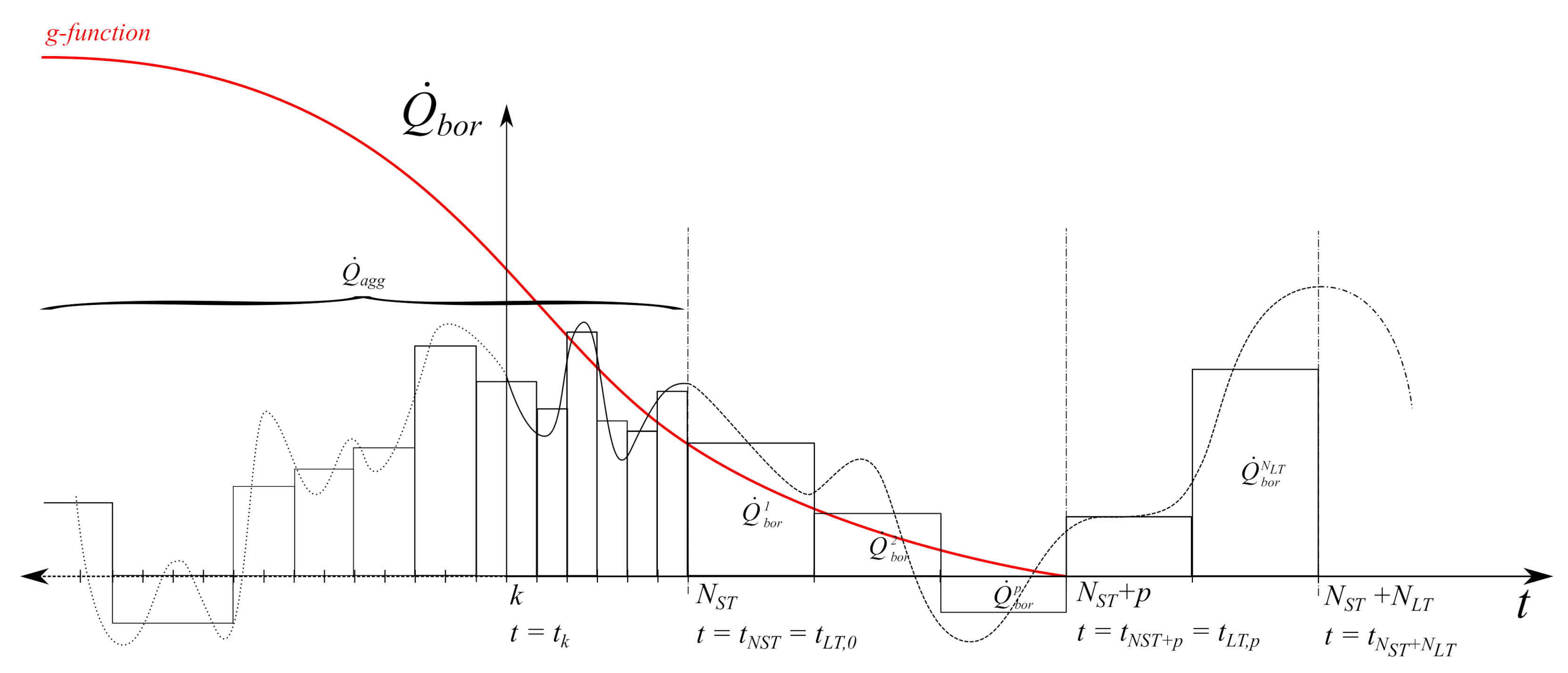
In the long-term, the ground dynamics are affected by the thermal interactions between different boreholes and the axial effects due to the finite length of each borehole. To account for these long-term effects, Eskilson [12] introduced the concept of borefield thermal response factors or ‘g-functions’, characteristic for a specific borefield geometry and selected ground properties. The g-functions represent the evolution of the average borehole wall temperature over time for a step heat extraction rate input. These g-functions can be analytically calculated in an accurate way using Finite Line Source (FLS) approximations and spatial superposition. The solution of the FLS problem can be computed in an efficient way using pygfunction [26], which follows the methods proposed by Cimmino and Bernier [27] and Cimmino [28]. A representation of a set of g-functions is given by Figure 1. Under a variable heat load, temporal superposition of the discretized ground load history of the borefield needs to be applied to compute the borehole wall temperature. Since the effects of a single load fade away with time, the load history further in the past can be aggregated in cells using aggregation schemes to reduce the computational cost [29,30]. At a given time-step k, each aggregated load proportionally contributes to the borehole wall temperature variation:
T b o r ( t k ) = T s + n = 1 n c Q ˙ a g g , n ( t k ) 2 π k s H b o r n b o r g ( τ a g g , n ) g ( τ a g g , n 1 ) = T s + n = 1 n c Q ˙ a g g , n κ a g g , n ,
where T b o r is the borehole wall temperature, T s is the undisturbed ground temperature, H b o r is the length of one individual borehole, n b o r is the number of boreholes, k s is the conductivity of the soil, Q ˙ a g g , n is the aggregated load at the n-th cell, n c is the total number of cells and τ is the time moving backwards through the load history starting at the k-th step such that τ a g g , n = t k t a g g , n and κ a g g , n is the weighting factor given by the difference of the g-functions evaluated at τ n and τ n 1 . The number of studies with focus on optimal control of geothermal systems that follow this approach is very limited, probably due to the complexity of modeling the cell-shifting phenomena across the aggregation cells in comparison to the approaches previously seen. Weeratunge et al. [31] modeled a single borehole using the infinite line source (ILS) solution [32] instead of the g-function in a solar-assisted configuration, disregarding however the short-term dynamics within the borehole. The work does not give details about whether a load-aggregation algorithm was used or the length of the considered load history. More recently, Laferrière and Cimmino [33,34] used a GSHP model represented by second-degree polynomial correlations and a borefield model that requires a discretized thermal response factor as input to compute the fluid temperature in a self-assisted water-to-air GSHP configuration, i.e., it uses a heating element on the source side of the GSHP to prevent too low operating fluid temperatures. Both works considered relatively short horizons of 5 days and 6 days respectively, for which the RC diffusion approximation is also suitable.
It can be concluded that most of the research in optimal control of geothermal systems is focused on the short-term dynamic aspects. Few authors have proposed formulations that take into account the long-term dynamics: Verhelst [13] proposed the introduction of a penalty cost in the objective function to the daily passive cooling budget, yet the weighting factor/cost for this term is not defined. Antonov [35] developed the Short-and-Long-Term-Optimization (SALTO) method, imposing yearly cyclic conditions on the ground nodes temperatures. However, although guaranteeing a sustainable use of the ground over the years, this approach may not be optimal as it curtails the freedom of MPC while a certain yearly imbalance can be allowed in the borefield depending on its size.

3. Proposed Methodology

The method of the shadow-cost aims to optimize the operation beyond the MPC prediction horizon, e.g., a full season/year, by using an estimation of the heating and cooling needs of the building. Section 3.1 describes the implementation of the shadow-cost in the MPC cost function. Section 3.2, Section 3.3 and Section 3.4 elaborate on how the estimations of the heating and cooling needs are used to define the building, energy system and borefield models that compute the long-term predictions necessary to calculate the shadow-cost. Finally, Section 3.5 formulates the shadow-cost.

3.1. Cost Function

To account for the long-term dynamics processes that occur in the ground (such as thermal interference between boreholes) in the optimization, we propose a reformulation of Equation (1), extending it by including a “shadow-cost”, equivalent to “long-term cost” or “cost of opportunity” in the cost function, such as:
min u k , u L T J = min u k , u L T k = 1 N S T J k + J L T = min u k , u L T J S T + J L T ,
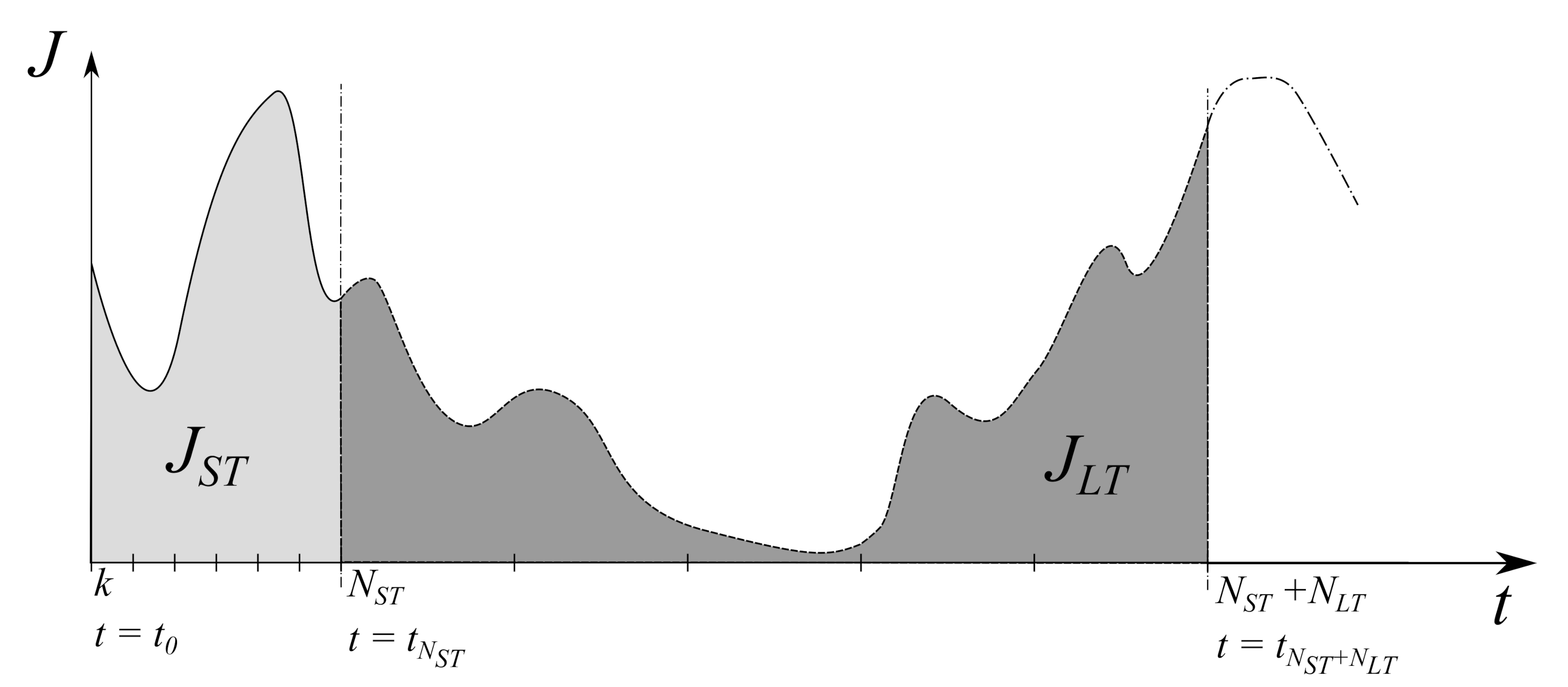
where J L T is the shadow-cost or long-term objective term and u L T are the optimization variables associated to this shadow-cost, while we denote the existing term in the optimization as the short-term objective J S T . The idea of the shadow-cost is to introduce an estimation of the objective cost starting from the end of the prediction horizon of the short-term optimization t N S T at the N S T step until a given longer period t N S T + N L T at the N S T + N L T step, e.g., a season or a full year, as depicted by Figure 2. A priori, an equivalent solution is to increase the prediction horizon length. However, a long prediction horizon is associated with an increased number of time-steps, thus increasing the number of all optimization variables and as a consequence the scale and complexity of the problem. Moreover, the longer the prediction horizon is, the higher the uncertainty there is related to the model and disturbance predictions: the prediction error of the building model increases with each time-step and not all information that the model requires (e.g., solar gains) is available in the long-term.

3.2. Building Long-Term Model

Since the weather predictions uncertainty is high, we need to rely on its seasonality and weather historical data as used for building design. This weather historical data could be calibrated with long-term seasonal predictions. Employing these rough weather projections, the future building heating and cooling needs could be estimated using for example a dynamic simulation or static methods, such as the heating or cooling degree-day method [36]. The long-term period considered to compute the shadow cost can be discretized in a number of long-term prediction steps, in the same way, the MPC short-term horizon is discretized in prediction time-steps. Assuming that the long-term prediction steps are sufficiently long so that the impact of the exact building dynamic behavior is diminished, for a building with n heat supply systems and m cold supply systems a steady-state building energy balance yields:
Q b u i , h p = i = 1 n Q i , h p
Q b u i , c p = j = 1 m Q j , c p p { 1 , , N L T }
where Q b u i , h p and Q b u i , c p are the pre-computed building heating and cooling energy needs, Q i , h p is the heating supplied by the i-th heat production system and Q j , c p is the cooling supplied by the j-th cold production system at the p-th long-term prediction step. The supplied heat and cold are subjected to capacity constraints as in Equation (1).

3.3. Energy System Long-Term Model

A heat/cold production system supplies thermal energy to the building by transforming an energy input according to its efficiency/performance over the considered period. Let J i , h p and J j , c p be the energy used by the i-th heat production system and the j-th cold production system at the p-th long-term prediction step, and η i , h p and η j , c p the efficiencies of the i-th heat production system and the j-th cold production system over the p-th prediction step. We have:
Q i , h p J i , h p = η i , h p
Q j , c p J j , c p = η j , c p p { 1 , , N L T }
In the particular case of a GSHP, its performance is quantified by the seasonal coefficient of performance (SCOP) for heating and the S E E R for cooling over the p-th long-term prediction step.
Q c o n p W c o m p = S C O P i p
Q e v a p W c o m p = S E E R j p p { 1 , , N L T } ,
where Q c o n p , Q e v a p and W c o m p are the energy supplied by the condenser, the energy absorbed by the evaporator and the energy used by the compressor, respectively. The S C O P and S E E R of the GSHP depend, among others, on the working fluid temperatures. Since the building long-term model is formulated using energy balance equations, it is not possible to determine the water supply temperature of the condenser. To account for the performance dependency on the temperature, a higher condenser temperature is expected for colder outdoor temperatures in heating regime and a lower evaporator temperature is expected for warmer outdoor temperatures in cooling regime. A dependency with the predicted average external temperature within the interval T e p is then assumed. Hence, the GSHP performances can be formulated using the following correlation:
S C O P i p = C 1 + C 2 T f p , n 1 + C 3 T e p , n 2
S E E R j p = C 4 + C 5 T f p , n 3 + C 6 T e p , n 4 p { 1 , , N L T } ,
where T f p and T e p are the average fluid temperature at the source side and external temperature predictions respectively at the p-th long-term prediction, n 1 , n 2 , n 3 , n 4 are the power coefficients that determine the order of the correlation and C 1 , C 2 , C 3 , C 4 , C 5 , C 6 are constants that depend on the used GSHP.

3.4. Borefield Long-Term Model

The fluid temperature at the source side is required to determine the GSHP performance. Moreover, this fluid temperature is constrained by the GSHP and passive cooling limits. It is assumed that the outlet of the geothermal borefield is connected to the inlet of the GSHP. From Equations (2) and (3) it is clear that the working fluid temperature depends on the load history of the borefield. In order to know the GSHP performances and the passive cooling capacity, the working fluid temperature needs to be estimated. Analogously to Equation (5), for ν components that can extract heat from the ground and μ components that can inject heat into the ground, an energy balance for the borefield side gives:
Q ˙ b o r p = i = 1 ν Q ˙ i , e x t p + j = 1 μ Q ˙ j , i n j p p { 1 , , N L T } ,
where Q ˙ b o r p is the average net heat load in the borefield, Q ˙ i , e x t p is the average extracted load by the i-th component (e.g., the GSHP evaporator, a dry cooler, etc.) and Q ˙ j , i n j p is the average injected load by the j-th component (e.g., the passive cooling heat exchanger, solar regeneration, etc.) over the p-th long-term prediction step. The sign convention is such that a load injection into the ground is positive and a load extraction from the ground is negative. Let t k be the discrete time in the short-term horizon, and t L T , q the discrete time in the long-term horizon at the q-th prediction, such that t N S T = t L T , 0 . We then have τ a g g , n = t k t a g g , n the time at the end of each cell in the aggregated load history, and in the long-term horizon we have τ L T , q = t L T , q t k at the q-th prediction. Applying temporal superposition, the p-th long-term prediction of the average borehole wall temperature difference is given by:
T b o r , L T p T s = n = 1 n c Q ˙ a g g , n ( t N S T ) 2 π k s H b o r n b o r g ( τ a g g , n + τ L T , p ) g ( τ a g g , n 1 + τ L T , p ) + q = 1 p Q ˙ b o r q 2 π k s H b o r n b o r g ( τ L T , p τ L T , q 1 ) g ( τ L T , p τ L T , q ) = n = 1 n c Q ˙ a g g , n ( t N S T ) κ S T , n p + q = 1 p Q ˙ b o r q κ L T , q p p 1 , 2 , , N L T
where the first term of the equation represents the average borehole wall temperature difference due to the complete short-term prediction horizon, while the second term represents the increase of the borehole wall temperature due to the superposition of the net heat energy borefield predictions. A graphical representation of Equation (10) is captured in Figure 3. The complete short-term prediction horizon is necessary to compute the long-term cost. Therefore, it is important to use the vector of aggregated loads at the last short-term horizon step k = N S T since otherwise there would be a ‘gap’ in the borefield load history. At each long-term prediction step, the vector of aggregated loads is further away in the past and its effect fades away with time. In essence, there is a different κ vector of weighting terms affecting each individual borefield load for each long-term prediction step. These extra κ vectors can be pre-computed prior to the optimization. In theory, a moving long-term prediction horizon strategy could be applied to account for the ‘gap’ between the vector of aggregated loads and the predicted loads and computing a shadow cost at each short-term optimization time-step. However, this would require the recomputation of the κ vectors at each short-term optimization step, increasing the computational burden of the optimization problem. Moreover, there is no point in doing so since the objective is to optimize the control inputs over the short-time horizon.
The borehole resistance R b o r can be used to calculate the average fluid temperature prediction at the p-th prediction T f p .
T f p = T b o r p + R b o r Q ˙ b o r p p { 1 , , N L T } .

3.5. Formulation of the Shadow-Cost

The shadow cost is formulated as:
J L T = p = 1 N L T i = 1 n c i p J i , h p + j = 1 m c j p J j , c p ,
where c i p and c j p are the weighting cost factors in line with the ones used in the short-term objective J S T at the p-th long-term prediction step. Adding this shadow cost to minimize the objective function involves the addition of m + n 2 long-term optimization variables u L T p per prediction step p, i.e., a total of ( m + n 2 ) N L T extra optimization variables, which can be a significant reduction compared to hypothetically extending the horizon. For passive cooling, the energy used by the circulation pump is considered.
In summary, the shadow cost long-term optimization and the building operation cost short-term optimization are coupled through the borefield model. The control actions of short-term optimization have an impact on the vector of aggregated loads Q ˙ a g g at the end of the short-term prediction horizon, which in turn has an impact on the long-term predictions of the fluid temperatures that are used to minimize the shadow cost.

4. Validation Case Study

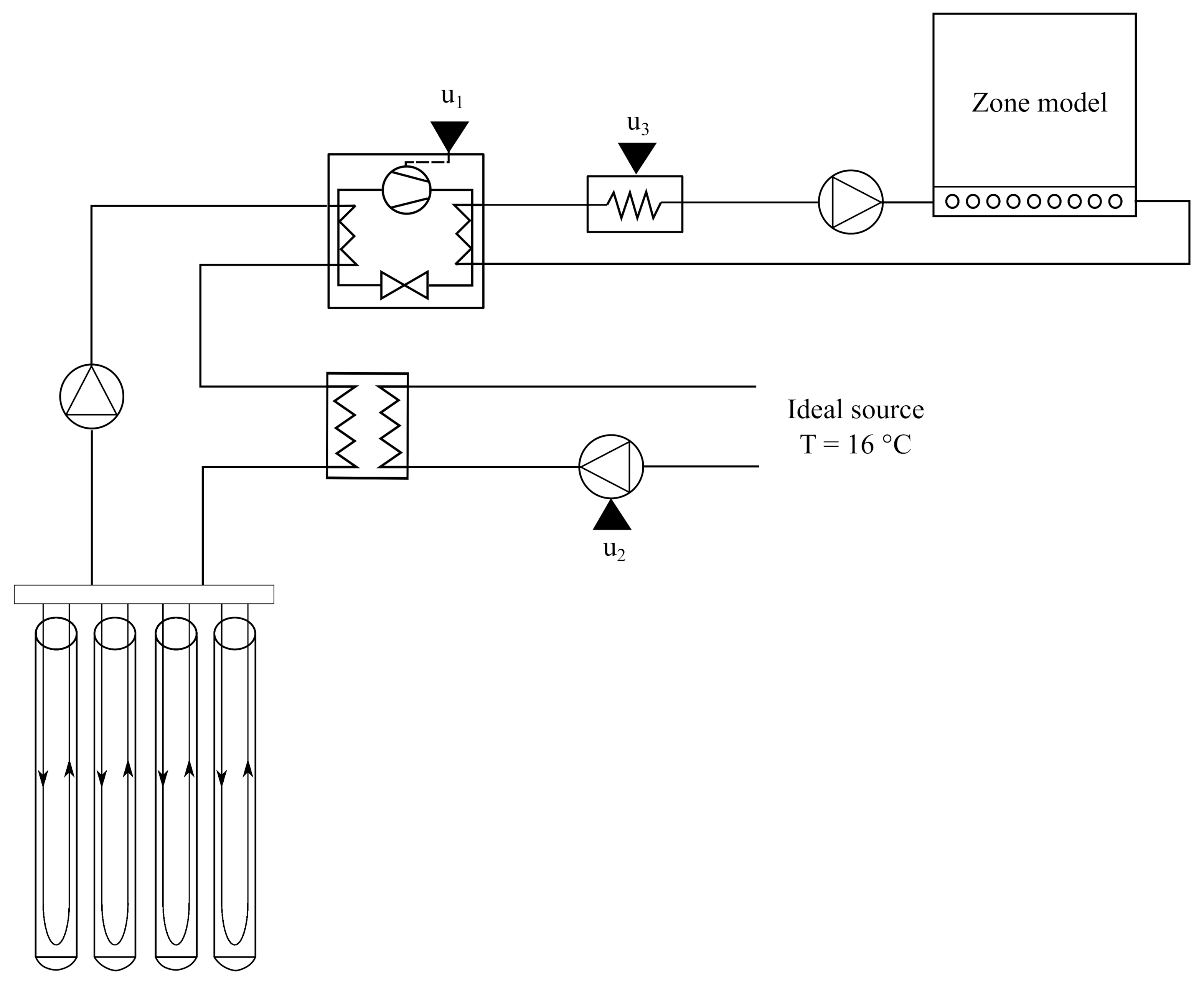
The proposed methodology is tested in the case study illustrated in Figure 4. A 1200 m 2 building, modeled as a single zone building, is equipped with a GSHP connected to an undersized borefield. An auxiliary electrical heating source is connected in series to the GSHP to provide extra heating during the peak hours. The heat is supplied to the building through an RHC embedded system. The building can regenerate the ground using a heat exchanger connected to an ideal source at a constant temperature of 16 C, however, the availability of this source is restricted to the summer months. In reality, this ideal source could represent an available heating source from solar collectors, waste heat, etc. No cooling system is installed in the building. The control input variables of the building include the GSHP modulation u 1 , the regeneration heat exchanger circulation pump signal u 2 and the auxiliary heating modulation u 3 signal. All signals are bounded between 0 and 1. The condenser and evaporator pumps operate at a constant rate.
Thermal comfort is guaranteed in the case study building using an MPC that delivers the control inputs that minimize the operational cost. The MPC optimization is performed at regular control time-steps of 1 h with a prediction horizon of 1 week. The first set of inputs of the optimal sequence is applied to the different components. The MPC framework used in this work can handle non-linear optimization problems (NLPs), provided that all equations are continuous and twice differentiable. Only time-based events are allowed. To facilitate the optimization process, only relevant non-linearities (such as the ones appearing in the Heating, Ventilation and Air Conditioning (HVAC) system) are kept in the optimization problem, while the non-relevant ones (such as the ones related to the building envelope, excluding solar radiation which is treated as an input) are linearized according to the work of Picard et al. [37]. As a consequence, the model used for simulation slightly differs from the model used for the optimization. Perfect state update from the simulation model to the optimization model is applied prior to each optimization to avoid error accumulation due to model mismatch. The building is assumed to be in Denver, Colorado and therefore the BESTEST TMY weather file is used, with extreme cold temperatures down to −24.4 C. There is no difference between the weather file used in the simulation model and the optimization model, implying perfect weather predictions. The different component models, as well as further details of the MPC formulation, are presented in the next subsections.

4.1. Building Envelope and Energy System Models

The models are constructed in the Modelica language [38] using verified component models from the IBPSA [39] and IDEAS [40] libraries. In practice, these models are calibrated using information from the real building. The building model corresponds to the IDEAS RectangularZone model, which assumes a perfectly mixed air volume within a rectangular construction geometry subjected to dynamic heat transfer relations. The zone temperature T z in the model is equal to the operative temperature given by the average of the air and radiant temperatures. The envelope is oriented towards south and the thermal characteristics of the construction can be found in Table 1. An equal number of windows is placed on each façade. The infiltration losses are computed based on an n 50 value of 0.5 ACH. Internal gains are accounted between 7 a.m. and 11 p.m. coming from 50 occupants at a heating rate of 73 W per occupant. Since the thermal mass of the building is large, it is decided not to take into account the re-heating load for the design load calculation. The building static design load according to the standard ISO12831 [41] is 40 kW when this re-heating load is not taken into account. The heat supply equipment is sized such that the GSHP capacity is 65% of this value and the auxiliary heating can provide 100%. The idea is that the GSHP is able to provide most of the energy while the auxiliary heating supports the GSHP during the peak hours. For the optimization, the building envelope is linearized using the methodology from Picard et al. [37].
The heat pump is non-reversible and modulating and its energetic performance relations are derived from an equation-fitting procedure based on a ClimateMaster TMW036 heat pump scaled to have a nominal capacity of 26 kW. However, this maximum capacity may vary depending on the GSHP operation conditions. Starting from the correlation defined by Cupeiro Figueroa et al. [23], we encountered some issues during the optimization as the fitted C O P tended to very high values at low modulation levels. Therefore, the condenser Q ˙ c o n and evaporator Q ˙ e v a capacities were chosen as the preferred variables to be fitted, while calculating the compressor power W ˙ c o m and the COP starting from these. In addition and for simplification, the temperature and modulation dependencies are kept linear in the correlations given by Equation (13).
Q ˙ c o n = A 1 + A 2 ( T e v a , i n T e v a , n o m ) + A 3 ( T c o n , i n T c o n , n o m ) u 1
Q ˙ e v a = B 1 + B 2 ( T e v a , i n T c o n , n o m ) + B 3 ( T c o n , i n T c o n , n o m ) u 1
W ˙ c o m = Q ˙ c o n Q ˙ e v a
C O P = Q ˙ c o n W ˙ c o m i f W ˙ c o m 0 1 i f W ˙ c o m = 0 ,
where T e v a , i n and T c o n , i n are the inlet fluid temperatures of the evaporator and condenser and T e v a , n o m and T c o n , n o m are the nominal temperatures of the evaporator and condenser respectively. The values of the fitted coefficients in Equation (13) are given in Table 2. The nominal condenser and evaporator temperatures are set at 35 C and 0 C respectively. The condenser and evaporator pumps work at a constant mass flow rate of 1.6 kg/s.
The borefield is comprised of 4 × 125 m single-U boreholes placed in a square configuration with a relative spacing of 6 m between adjacent boreholes. Further details on the borefield parameters are given in Table 3. The borefield model is based on the borefield model developed by Picard and Helsen [42] and refined by Laferrière et al. [43] for the IBPSA library. The heat transfer process within the borehole is axially discretized. A thermal-capacity network is used to model the radial heat transfer and the fluid nodes at each discretization are connected with advection heat transfer equations. The ground response is modeled using temporal superposition as defined by Equation (3). The load-shifting algorithm is modified from an event-based formulation to a continuous one using a QUICK (Quadratic Upstream Interpolation of Convective Kinetics) method [44] as presented in Equation (14), so that the MPC NLP solver is able to handle it.
d Q ˙ a g g , n d t = Q ˙ a g g , n 1 / 2 Q ˙ a g g , n + 1 / 2 Δ τ n
Q ˙ a g g , n 1 / 2 = Q ˙ a g g , n 1 + Q ˙ a g g , n 2 ( τ n τ n 1 ) 2 8 Δ τ n 1 Q ˙ a g g , n Q ˙ a g g , n 1 τ n τ n 1 Q ˙ a g g , n 1 Q ˙ a g g , n 2 τ n 1 τ n 2
Q ˙ a g g , n + 1 / 2 = Q ˙ a g g , n + Q ˙ a g g , n + 1 2 ( τ n + 1 τ n ) 2 8 Δ τ n Q ˙ a g g , n + 1 Q ˙ a g g , n τ n + 1 τ n Q ˙ a g g , n Q ˙ a g g , n 1 τ n τ n 1
Q ˙ a g g , 1 / 2 = Q ˙ b o r ,
where Q ˙ b o r is the heat load injected/extracted into/from the ground, Q ˙ a g g , n is the aggregated load in the n-th aggregation cell, and Q ˙ a g g , n 1 / 2 and Q ˙ a g g , n + 1 / 2 are the interpolated loads at the left and right faces of the n-th load aggregation cell, respectively. The borefield g-function is prescribed as a separate input file precomputed using the Python package pygfunction [26], based on the methods of Cimmino and Bernier [27] and Cimmino [28]. The ground response model is slightly modified to include the wall temperature predictions, implementing the long-term temporal superposition algorithm described in Equation (10) and require an array of predicted long-term borefield loads.
The heat exchanger is a counter-flow plate heat exchanger with a heat transfer coefficient U A listed in Table 4. The computation of the heat transfer rate is based on the NTU-epsilon method [45]. For a counter-flow heat exchanger, Equation (15) holds.
C r = C m i n C m a x
N T U = U A C m i n
ϵ = 1 e N T U ( 1 C r ) 1 C r e N T U ( 1 C r )
Q ˙ h e x = ϵ C m i n ( T h e x , h o t , i n T h e x , c o l d , i n )
where C m i n and C m a x are the minimum and maximum heat capacity rates, C r is the heat capacity ratio, N T U is the number of transfer units, ϵ is the effectiveness of the heat exchanger and T h e x , h o t , i n and T h e x , c o l d , i n are the inlet temperatures in the heat exchanger both at the hot and the cold side. The circulation pump model corresponds to the one from the IBPSA library based on similarity laws [46]. The modulation signal can set the pressure drop input of the pump Δ p h e x to overcome the pressure loss in the regeneration heat exchanger. Consequently, the mass flow rate in the regeneration heat exchanger m ˙ is calculated using a flow coefficient k in Equation (16). The flow coefficient is calculated using the nominal parameters from Table 4. Since the ideal source is only available during the summer months, the optimization variable of the regeneration pump u 2 is multiplied by a time-dependent variable Ψ that allows its operation during that period only. To compute the electric power, the default curve and efficiencies of the model are used. Essentially, the pump electric power W p u m cubically increases with the mass flow rate up to its nominal power W p u m , n o m :
Ψ u 2 Δ p n o m = m ˙ k 2
W ˙ p u m = Ψ u 2 3 W ˙ p u m , n o m
Finally, the auxiliary electric heater model is assumed to supply heating in a linear relation to its modulation signal. It is assumed that it transforms electricity into heat with 100% efficiency.
Q ˙ a u x = u 3 Q ˙ a u x , n o m
W ˙ a u x = Q ˙ a u x .

4.2. Control Strategies

The described model is extended with the optimization specifications using Optimica [47] and translated into an optimization problem using TACO [48]. The implementation of the NLP is made through CasADi [49]. An external C-code links the optimal control inputs resulting from the optimization to the model during the simulation.
The building heating system operates to keep the zone temperature T z given by the IDEAS zone model equations higher than a pre-set lower comfort bound T z ̲ that follows a night set-back profile. During the day, when the building is occupied, the limit is set at 21 C while at night the bound is reduced to 16 C. Three MPC strategies, differing in the way regeneration is controlled, are tested:
  • A state-of-the-art MPC for the whole system;
  • A state-of-the-art MPC combined with an RBC that activates the regeneration pump during the summer period, i.e., maximizes the amount of regenerated heat;
  • An MPC that includes the shadow-cost methodology.
The horizon is divided in 14 N S T intervals, structured as depicted in Table 5. Perfect state updates and perfect weather predictions are assumed, avoiding uncertainties from these aspects. The first strategy comprises a full MPC scenario that aims to minimize the operational costs of the installation according to the formulation given by Equation (18).
min u k J 1 = min u k k = 1 N S T c e l W ˙ c o m , k + W ˙ a u x , k + W ˙ p u m , k + s = 1 S 1 σ s , k Δ t k
σ 1 = c σ 1 ( T z ̲ T z ) 2 i f T z ̲ > T z 0 i f T z ̲ T z
σ 2 = c σ 2 ( T e v a , o u t ̲ T e v a , o u t ) 2 i f T e v a , o u t ̲ > T e v a , o u t 0 i f T e v a , o u t ̲ T e v a , o u t ,
where T e v a , o u t is the outlet fluid temperature of the evaporator, T e v a , o u t ̲ is the safety minimum temperature constraint of the GSHP, and c e l is the electricity price. The GSHP safety constraint is set at 0 C and the electricity price at 0.204 $/kWh. A set of S 1 quadratic penalization costs σ s are introduced to keep (i) the comfort limits in the building and (ii) the temperature operation range within the GSHP evaporator, and weighted with a scaling factor to speed-up the optimization c σ s .
In the second strategy, the pumping power of the regeneration heat exchanger W ˙ p u m is removed from the objective function in Equation (18) and this component is now controlled by a traditional rule-based controller (RBC). In the period where regeneration is possible, the pump operates at nominal conditions.
The third strategy follows an MPC approach similar to the first one, but with the addition of the shadow cost term. The optimization problem uses the building heating energy needs computed from a previous simulation as input. The long-term horizon comprises a full year divided in 14 N L T long-term prediction steps, structured as presented in Table 5: the first three steps have a weekly resolution up to the first month, while the remaining 11 steps cover the rest of the year with monthly steps. Therefore, for each long-term prediction step p the energy balances for both the building and the borefield yield:
Q b u i , h p = Q c o n p + Q a u x p
Q ˙ b o r p Δ t p = S C O P p 1 S C O P p Q c o n p + Q h e x p ,
where Δ t p is the size of the p-th long-term interval. The first term in Equation (19) for Q ˙ b o r p represents the predicted evaporator energy, which coincides with the extracted heat energy from the ground, and the second term represents the heat injected into the ground as a result of the regeneration heat exchanger. To compute the COP on the long-term, we assume a linear relation with the borefield predicted fluid temperature T f p calculated using Equations (10) and (11), and the average external temperature prediction T e p . The coefficients can be found in Table 2.
S C O P p = C 1 + C 2 T f p + C 3 T e p .
Equations (13) and (17) are used to compute the predictions of the compressor and auxiliary power. The regeneration heat exchanger flow can be computed using Equation (15) for each p-th long-term prediction step, where T h e x , h o t , i n is the ideal source temperature of 16 C and T h e x , c o l d , i n coincides with the predicted fluid temperature T f p . Then, applying Equation (16) the pump electrical power can be predicted. The shadow cost can be formulated as:
J L T = p = 1 N L T c e l W ˙ c o m p + W ˙ a u x p + W ˙ p u m p + s = 1 S 2 σ L T s Δ t p ,
and the MPC is formulated as:
min u k J 3 = min u k ( J 1 + J L T )
σ L T 1 = c σ L T 1 p = 1 N L T ( Q ˙ c o n p ) 2 i f Q ˙ c o n p < 0 c σ L T 1 p = 1 N L T ( Q ˙ c o n p Q ˙ c o n ¯ ) 2 i f Q ˙ c o n p > Q ˙ c o n ¯ 0 i f 0 Q ˙ c o n p Q ˙ c o n ¯
σ L T 2 = c σ L T 2 p = 1 N L T ( Q ˙ a u x p ) 2 i f Q ˙ a u x p < 0 c σ L T 2 p = 1 N L T ( Q ˙ a u x p Q ˙ a u x ¯ ) 2 i f Q ˙ a u x p > Q ˙ a u x ¯ 0 i f 0 Q ˙ a u x p Q ˙ a u x ¯
σ L T 3 = c σ L T 3 p = 1 N L T ( Q ˙ h e x p ) 2 i f Q ˙ h e x p < 0 c σ L T 3 p = 1 N L T ( Q ˙ h e x p Q ˙ h e x ¯ ) 2 i f Q ˙ h e x p > Q ˙ h e x ¯ 0 i f 0 Q ˙ h e x p Q ˙ h e x ¯
σ L T 4 = c σ L T 4 p = 1 N L T ( T f p T f ̲ ) 2 i f T f p > T f ̲ 0 i f T f ̲ T f p ,
where Q ˙ c o n ¯ , Q ˙ a u x ¯ and Q ˙ h e x ¯ are the capacity limits of the GSHP, auxiliary system and regeneration heat exchanger, and T f ̲ is the safety average temperature constraint at the source side of the GSHP. An additional set S 2 of long-term quadratic penalization terms σ L T is added to the problem formulation. Penalizations in Equation (22) ensure that the power distribution resulting from the optimization is within the system capacity limits. The capacity limits of the GSHP and auxiliary system are given by the nominal values in Table 4, while the capacity limit for the heat exchanger is given by Equation (15) with ϵ = 1 . Analogous to Equation (18), the penalization term σ L T 4 ensures that the fluid is within the temperature range of the GSHP. However, in this case the constraint T f ̲ is set at 0.75 C as it is the mean fluid temperature.

5. Results and Discussion

5.1. Comparison of Control Strategies

The case study is simulated for a 10-year long period starting at the beginning of the winter season, using an Euler integrator with a variable time-step of 15 s, i.e., the time-step can become shorter if an event (e.g., change in a control input condition) is triggered. After each hour and following the described MPC strategies, the cost-optimization is solved and a new set of inputs is prescribed to the simulation. The weather data file range comprises one full year, therefore these forecasts are repeated each year.
The results in Table 6 show a negligible use of the regeneration pump in the strategy with full MPC control (i.e., strategy 1). In summer, heat injection into the borefield is usually detrimental to the system operational costs over the short-term horizon, so MPC tends to not use it. Among the three strategies, strategy 2 is able to maximize the use of the GSHP and minimize the use of the auxiliary system by injecting the highest amount of energy into the ground. Despite this, the cost savings by the increased GSHP use are not able to offset the cost savings from the regeneration pump in strategy 3. In essence, strategy 2 could be seen as an upper bound to the energy actively regenerated into the borefield since regeneration is applied whenever possible, whereas strategy 3 regenerates energy in a cost-effective way over the considered long-term horizon. Comparing strategy 2 against strategy 3, the energy used by the regeneration pump is increased by almost a factor 9, while the regenerated energy only increased by 7.7% and the energy use of the GSHP by 0.6%. The regenerated energy/pump energy use ratio is far higher for strategy 3. The SCOP shows a slight increase in the order of the second decimal since the GSHP is typically working at the evaporator temperature limit in all cases. The shadow cost formulation (i.e., strategy 3) is able to reduce the operational costs by 9.7% when compared to strategy 1 and by 4.9% when compared to strategy 2. The main drawback is the increase in computational time by about a factor 3.5.
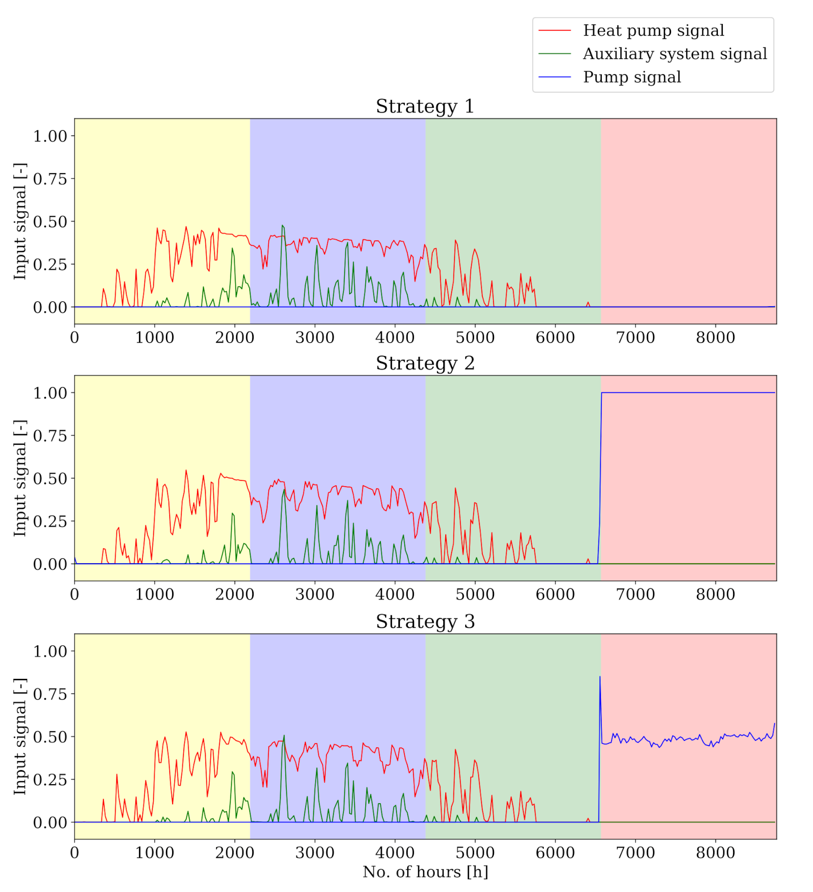
The behavior of the control input variables for a typical year is represented in Figure 5 using their daily average values. Strategy 1 rarely uses the regeneration pump during the allowed period (summer/red background), as the MPC cannot appreciate any benefit of using the regeneration pump within its short prediction horizon. At the end of the summer season, when the short-term horizon (1 week) can start predicting the future heating needs, there is a timid but late use of the regeneration pump. The regeneration pump signal of strategy 3 halves the one of strategy 2, incurring much less energy use from the pump. An oscillatory behavior in the regeneration pump is observed for strategy 3. These oscillations are likely caused by the small impact of the pumping cost during the 1 h control time step in the yearly cost objective. As a consequence, it is difficult for the NLP solver to find a smooth optimum at the selected tolerance settings. At the end of the summer season, the pump signal slightly increases in strategy 3, in order to increase the fluid temperature and maximize the COP in the heating season that starts in the short term.
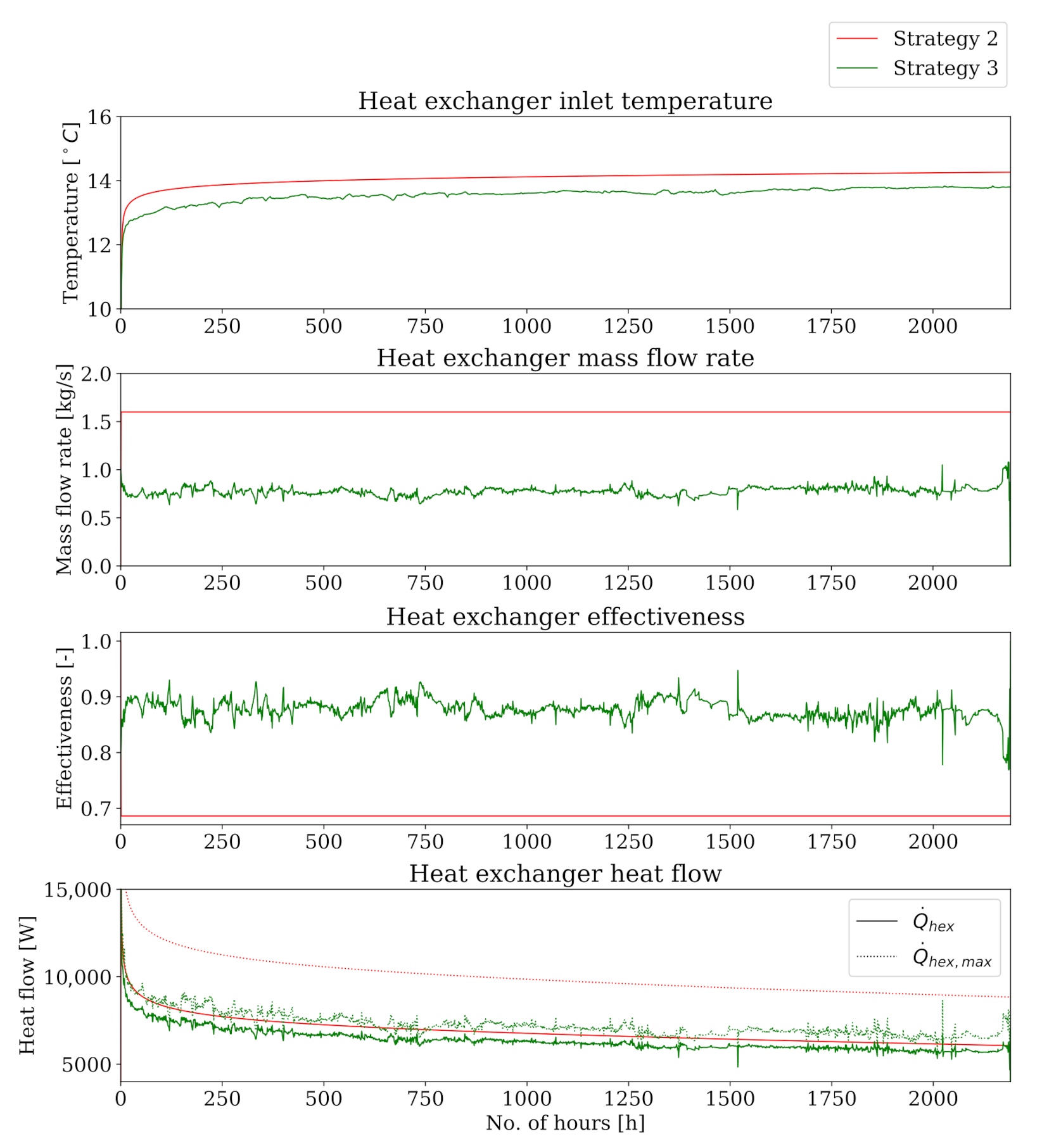
A closer look at the regeneration heat exchanger variables for strategies 2 and 3 during the summer season are shown in Figure 6. From Equation (15), it is known that the maximum heat exchange is determined by the inlet temperature difference, minimum heat capacity rates and a unitary effectiveness. By using a lower signal, the mass flow rate and, as a consequence, the heat capacity rate of strategy 3 decreases. However, this effect is modestly mitigated by the fact that the inlet temperature in the heat exchanger at the borefield side decreases. On the other hand, by decreasing the heat capacity rate of the heat exchanger the number of transfer units N T U increases, therefore increasing the heat exchanger effectiveness ϵ . Consequently, the actual heat transfer occurring within the heat exchanger is similar for the two strategies, while strategy 3 uses much less pumping power.
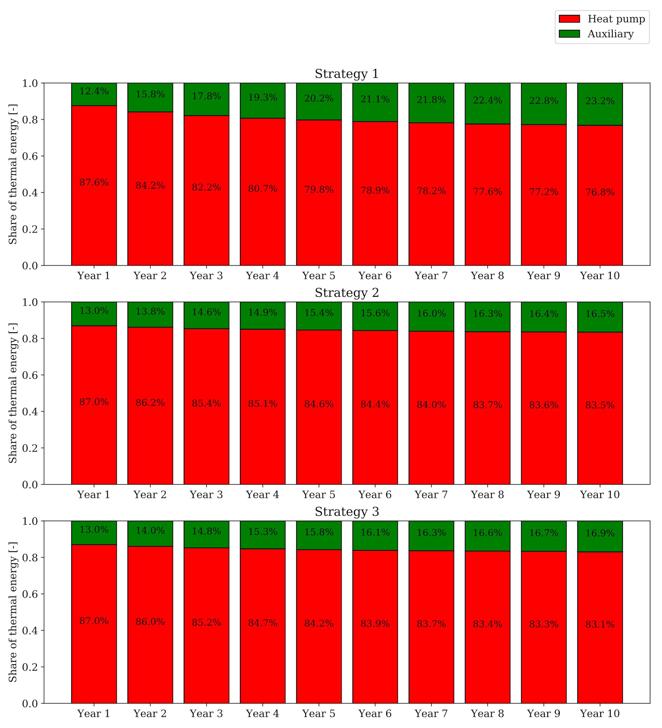
Figure 7 shows the yearly distribution of the thermal energy in the building while Figure 8 shows the yearly distribution of the operational costs as well as the accumulated costs over the simulation period. Since there is no ground regeneration in strategy 1, the share of the GSHP decreases after each year, while strategies 2 and 3 are able to abate this thermal depletion. As a consequence, and despite having a smaller operational cost in the first year, the costs of strategy 1 increase after each year as the borefield is more and more depleted, necessitating the use of the auxiliary system. The cost of heating the building are lower for strategy 2, yet by adding the regeneration cost the total yearly cost is higher for strategy 2 than for strategy 3. The regeneration pumping cost represents between 5.6–5.9% of the yearly cost in strategy 2 and 0.7% in strategy 3. Compared to strategy 1, it is not until the fourth year that the cost savings of strategy 2 begin to be noticeable, while in strategy 3 the return on investment of using the regeneration pump is apparent already from the second year.

5.2. Effect of Different Long-Term Horizons

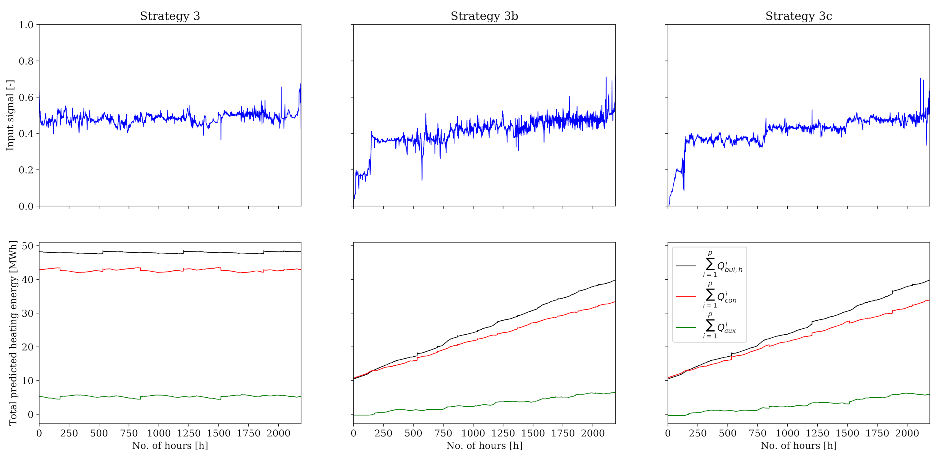
The model is now used to assess the impact of the shadow cost long-term horizon on the results. Strategy 3 is thus modified both in terms of long-term horizon length and resolution. Strategy 3b reduces from a yearly long-term horizon to a seasonal one, i.e., 6 months. Strategy 3c considers the same seasonal horizon length as 3b, but reducing the number of long-term intervals N L T from 14 to 8. The modified strategies are summarized in Table 7.
Table 8 compares the results for these variations in the long-term prediction horizon parameters. As expected, Strategy 3 is able to achieve the lowest operational cost since it is able to anticipate the full yearly needs, followed by Strategy 3b which has more resolution compared to Strategy 3c. However, the operational cost reduction by capturing the cyclic yearly heating needs is more noticeable (difference between Strategies 3 and 3b) than increasing the resolution of the horizon (difference between Strategies 3b and 3c). By lowering the long-term horizon resolution, we observe a clear reduction of the computational cost: the average number of iterations is reduced by 16.3% and the average time per iteration by 13.8%. This computation time reduction is mainly caused by the reduction of the number of optimization variables associated with each additional interval. Each additional long-term optimization variable will have a dependency on all the previous ones, increasing the complexity of the problem. Moreover, TACO optimization variables are defined for the whole prediction horizon resolution, while in practice only the values at the last step of the short-term prediction horizon are used for the energy balance calculations. In that sense, the computational time could be possibly reduced with a different implementation. However, TACO does not provide enough information on the computational metrics to confirm this hypothesis. From this perspective, we recommend to use a long-term horizon large enough to capture the building cyclic conditions but with the smallest possible number of intervals (i.e., resolution). All three scenarios (3, 3b, 3c) have a lower operational cost than strategies 1 and 2. Thus, including the shadow cost in the objective function leads to a decrease in operational costs in all studied cases.
Figure 9 compares the regeneration pump input signals along with the total predicted heat supply distribution of the building for the last summer season. Strategies 3b and 3c signals tend to increase over the summer period, in accordance with the total predicted building heating energy. The long-term horizon covers an increasing fraction of the next season, so it is increasingly beneficial to regenerate the soil. Strategy 3 always covers the full heating season, so the signal is flatter. At the beginning of the summer season, Strategies 3b and 3c predict that the building heating needs are small enough to supply all the necessary heating with the GSHP by applying a small amount of active regeneration to the ground. However, these heating needs increase over the season to the point where the auxiliary system needs to cover the remaining predicted amount of heat energy supply. As a consequence, not enough regeneration energy is injected into the ground. Note that the step changes in the plot are caused by the time-dependent variable Ψ , and are more noticeable in Strategy 3c as it has larger but more impactful intervals.

5.3. Effect of the Predictions Accuracy

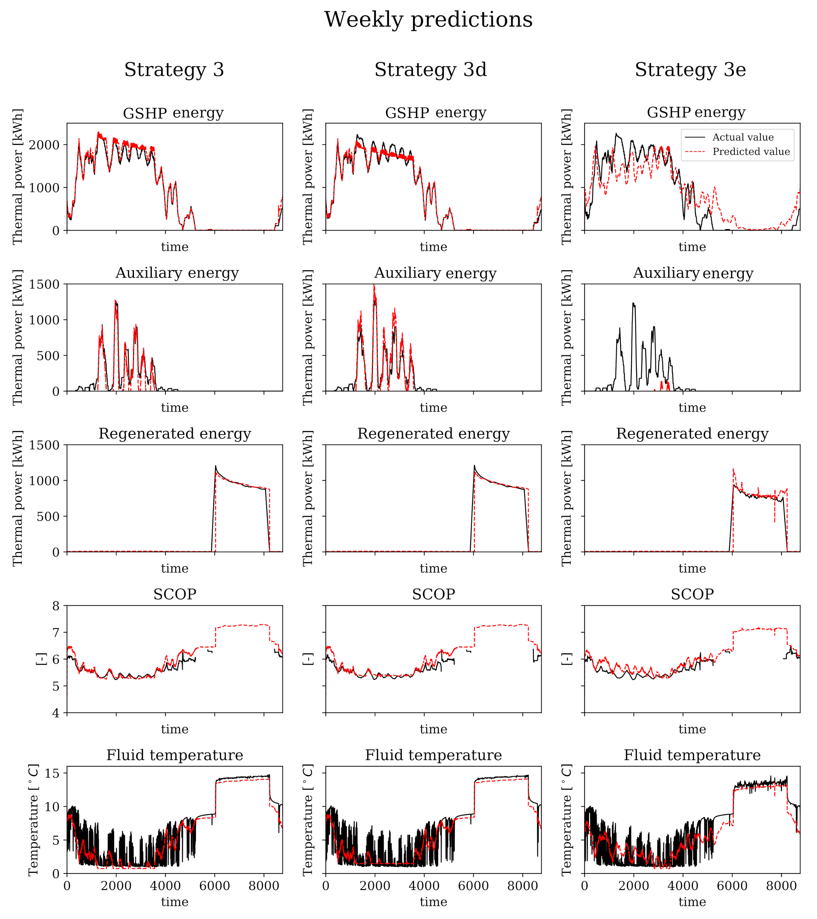
The previous simulations with shadow cost use a prescribed set of building heating needs coming from an offline dynamic simulation that uses the same weather file, thus having relatively accurate predictions. In reality, these weather predictions will have a large uncertainty, yet an estimation of the energy needs of the building can be obtained using historical weather data and a static method such as the degree-days method. Additionally, weather services provide long-term seasonal forecasts that indicate whether the next season is expected to be warmer or colder than usual, thus allowing extra tuning of the building load needs accordingly. On the other hand, the prediction of the average fluid temperature limits the amount of energy that can be provided by the GSHP. Based on the observations from Section 5.2, the prediction accuracy of this parameter can have an impact on the final outcome. Two extra simulations are therefore carried out: a simulation 3d with a different long-term fluid temperature constraint T f ̲ = 1.5 C; and a simulation 3e with a different set of prescribed building heating needs, extracted from the heating degree-day information for the year 2019 in the city of Denver [50]. The HDD data is used for the long-term predictions, but still the TMY data from the previous strategies is used for simulation.
Results of these simulations are shown in Table 9. Strategy 3d injects more heat into the ground but, at the same time, the amount of condensing energy from the GSHP is reduced. This may be caused by an overestimation of the average fluid temperature, which causes the control strategy to be on the conservative side. However, the impact on the results is not significant. On the other hand, Strategy 3e has a significant reduction of the injected energy into the ground, which results in increased use of the auxiliary heating system. The reason is the underestimation of the required heating needs: the prescribed heating needs for strategy 3e are 43 MWh per year, about 10% lower compared to the 48 MWh per year of the previous strategies.
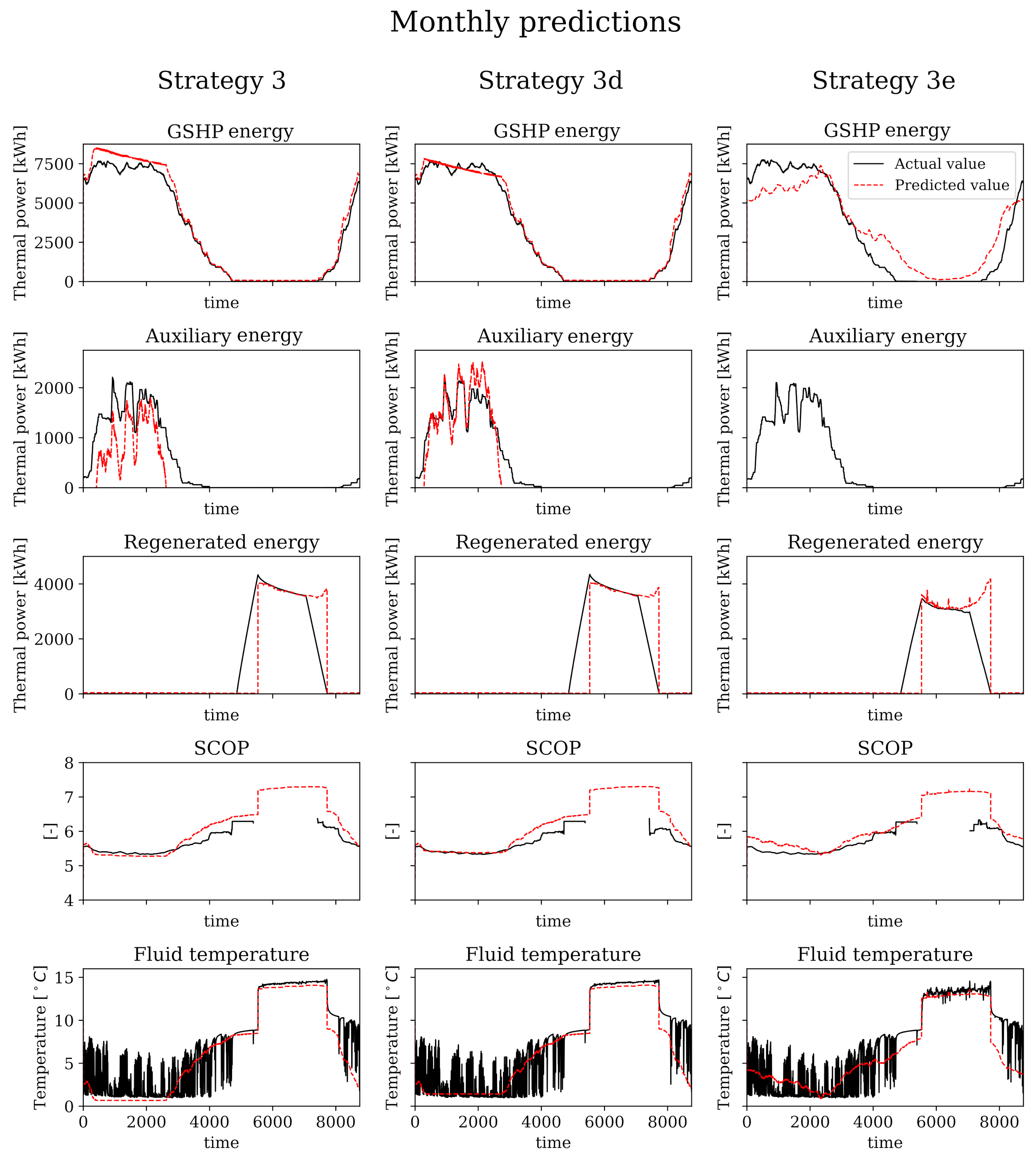
Figure 10 and Figure 11 compare the first weekly and monthly predictions with the actual shifted results for one year, and confirm the aforementioned hypothesis. The overestimation of the average fluid temperature constraint in Strategy 3d causes that the predicted amount of heating delivered by the GSHP is lower than the one from Strategy 3, driving the optimization towards an increased use of the auxiliary system. Increasing the amount of active regeneration does not seem to be the optimal choice. The heating predictions from Strategy 3e cause the system to provide a lower amount of active regeneration, since based on the simplified (HDD-based) heating needs prediction it would suffice to satisfy almost all of the heating requirements with the GSHP. Strategy 3e predicts almost no use of the auxiliary system. These incorrect predictions ultimately have a negative impact in the final result. Still, these strategies lead to lower cost compared to strategies 1 and 2, again confirming the added value of including the shadow cost in the objective function.

6. Conclusions

This paper presents a novel methodology to account for the long-term effects of the geothermal borefield in hybrid geothermal installations that use MPC. The objective function is extended with a shadow cost that represents the cost of opportunity in the period not accounted in the MPC short-term prediction horizon. The shadow cost is calculated using prescribed predictions of the building heating and cooling needs and imposing energy balance equations for the different supply components of the system. These long-term predictions can be discretized in several intervals in the same way as the MPC short-term prediction horizon. The MPC and the shadow cost are connected through the load history of the borefield model. As a consequence, the actions of the MPC modestly affect the shadow cost calculation.
The methodology is verified in a single zone building of 1200 m 2 that is equipped with a hybrid geothermal system and an ideal regeneration system that can only be used in the summer period, i.e., when heating is not needed in the building. Three different control strategies are compared: an MPC approach, an MPC + RBC for the regeneration system approach and an MPC + shadow cost approach. Results show that the MPC + shadow cost approach is able to optimally use the active regeneration, minimizing the pumping cost and reducing the total operational cost over 10 years by 9.7% when compared to the MPC approach and 4.9% when compared to the MPC + RBC approach. However, the shadow cost approach increases the computational time by a factor of 3.5. The effects of the long-term horizon length and resolution are analyzed. It is concluded that it is important to have a long-term horizon that captures the cyclic heating and cooling needs of the building, but with a limited number of steps to reduce the computational cost. The effect of the prediction accuracy is also investigated. An overestimation of the minimum fluid temperature constraint causes increased use of the auxiliary system. An underestimation of the building heating needs causes a reduced use of the active regeneration, leading to increased use of the auxiliary system. For this specific case, the impact on the operational cost is not substantial but this cannot be generalized, so attention should be paid. Even with these inaccuracies, the shadow cost formulation achieves greater cost savings than the formulations where it was not used.
This methodology fills the gap in the literature towards the optimization of the operation of geothermal systems over a full year, introducing a novel long-term shadow-cost formulation and demonstrating that there is potential for savings from a MPC approach integrating yearly costs in the optimization. Even with the known drawback that the building needs prediction uncertainty is high in the long-term, the methodology still outperforms in cost-saving terms the pure MPC (no regeneration) and the combined RBC + MPC (maximum regeneration) cases even when a standard historical method, such as the degree-day method, was used.
Further work should reduce these uncertainties using other methods or meteorological models. Moreover, it should be investigated where the application of this methodology is most beneficial. Potentially, all hybrid GSHP systems could benefit from this methodology, but also systems where a seasonal optimal planning is of interest, such as solar systems, district heating systems, thermal energy storage systems and other systems where the time constant is long. The methodology could also be included in an integrated optimal design and control framework, where the optimal long-term control actions are taken into consideration to reduce the total amount of investment and operational costs over the considered lifetime. Finally, a smarter implementation of the methodology in the MPC framework should be investigated to reduce the computational burden.

Author Contributions

Conceptualization, I.C.F. and M.C.; methodology, I.C.F. and M.C.; software, I.C.F.; validation, I.C.F.; formal analysis, I.C.F.; investigation, I.C.F.; resources, M.C. and L.H.; data curation, I.C.F.; writing—original draft preparation, I.C.F.; writing—review and editing, M.C. and L.H; visualization, I.C.F.; supervision, M.C. and L.H.; project administration, L.H.; funding acquisition, I.C.F. and L.H. All authors have read and agreed to the published version of the manuscript.

Funding

The authors would like to acknowledge the funding of their research work by the EU within the H2020-EE-2016-RIA-IA programme for the project ‘Model Predictive Control and Innovative System Integration of GEOTABS-; in Hybrid Low Grade Thermal Energy Systems-Hybrid MPC GEOTABS’ [grant number 723649-MPC-; GT]. The authors would like to acknowledge the InnoEnergy PhD School Programme and the European Institute of Technology (EIT) for supporting the international mobility from which this work was emerged.

Acknowledgments

This work emerged from the IBPSA Project 1, an international project conducted under the umbrella of the International Building Performance Simulation Association (IBPSA). Project 1 will develop and demonstrate a BIM/GIS and Modelica Framework for building and community energy system design and operation.

Conflicts of Interest

The authors declare no conflict of interest.

Abbreviations

The following abbreviations are used in this manuscript:
ANNArtificial neural network
COPCoefficient of performance
DSTDuct-storage model
EEREnergy efficienct ratio
GSHPGround source heat pump
HVACHeating, ventilation and air conditioning
LPLinear problem
MILPMixed integer linear problem
MPCModel predictive control
MORModel order reduction
NLPNon-linear problem
NTUNumber of transfer units
OCPOptimal control problem
PODProper orthogonal decomposition
QUICKQuadratic upstream interpolation of convective kinetics
TABSThermally activated building systems
RBCRule based control
RCResistance-capacitance
RHCRadiant heating and cooling
SALTOShort- and long-term optimization
SCOPSeasonal coefficient of performance
SEERSeasonal energy efficiency ratio
TACOToolchain for automated control and optimization

References

  1. De Coninck, R.; Helsen, L. Practical implementation and evaluation of model predictive control for an office building in Brussels. Energy Build. 2016, 111, 290–298. [Google Scholar] [CrossRef]
  2. Vana, Z.; Cigler, J.; Siroky, J.; Zacekova, E.; Ferkl, L. Model-based energy efficient control applied to an office ock. J. Process Control 2014, 24, 790–797. [Google Scholar] [CrossRef]
  3. West, S.R.; Ward, J.K.; Wall, J. Trial results from a model predictive control and optimisation system for commercial building HVAC. Energy Build. 2014, 72, 271–279. [Google Scholar] [CrossRef]
  4. Camacho, E.F.; Alba, C.B. Model Predictive Control; Springer: Berlin/Heidelberg, Germany, 2013. [Google Scholar]
  5. Cupeiro Figueroa, I.; Cigler, J.; Helsen, L. Model Predictive Control formulation: A review with focus on hybrid GEOTABS buildings. In Proceedings of the REHVA Annual Meeting Conference Low Carbon Technologies in HVAC, Brussels, Belgium, 24 April 2018; pp. 1–9. [Google Scholar]
  6. Himpe, E.; Vercautere, M.; Boydens, W.; Helsen, L.; Laverge, J. GEOTABS concept and design: State-of-the-art, challenges and solutions. In Proceedings of the REHVA Annual Meeting Conference Low Carbon Technologies in HVAC, Brussels, Belgium, 24 April 2018. [Google Scholar]
  7. ASHRAE. Chapter 34: Geothermal Energy. In ASHRAE Handbook: Applications; American Society of Heating, Refrigerating and Air-Conditioning Engineers: Atlanta, GA, USA, 2015. [Google Scholar]
  8. Bernier, M.A. Closed-loop ground-coupled heat pump systems. Ashrae J. 2006, 48, 12–25. [Google Scholar]
  9. Atam, E.; Helsen, L. Ground-coupled heat pumps: Part 1—Literature review and research challenges in modeling and optimal control. Renew. Sustain. Energy Rev. 2016, 54, 1653–1667. [Google Scholar] [CrossRef]
  10. Hellström, G. Duct Ground Heat Storage Model, Manual for Computer Code; Department of Mathematical Physics, University of Lund: Lund, Sweden, 1989. [Google Scholar]
  11. Verhelst, C.; Helsen, L. Low-order state space models for borehole heat exchangers. HVAC R Res. 2011, 17, 928–947. [Google Scholar] [CrossRef]
  12. Eskilson, P. Thermal Analysis of Heat Extraction Boreholes. Ph.D. Thesis, University of Lund, Lund, Sweden, 1987. [Google Scholar]
  13. Verhelst, C. Model Predictive Control of Ground Coupled Heat Pump Systems for Office Buildings. Ph.D. Thesis, Katholieke University Leuven, Leuven, Belgium, 2012. [Google Scholar]
  14. Atam, E.; Verhelst, C.; Helsen, L. Development of a control-oriented model for borehole dynamics for buildings equipped with ground-coupled heat pumps. In Proceedings of the 13th Conference International Building Performance Simulation Association (BS 2013), Chambéry, France, 25–28 August 2013; pp. 2052–2059. [Google Scholar]
  15. Atam, E.; Helsen, L. A convex approach to a class of non-convex building HVAC control problems: Illustration by two case studies. Energy Build. 2015, 93, 269–281. [Google Scholar] [CrossRef] [Green Version]
  16. Atam, E.; Patteeuw, D.; Antonov, S.P.; Helsen, L. Optimal control approaches for analysis of energy use minimization of hybrid ground-coupled heat pump systems. IEEE Trans. Control Syst. Technol. 2015, 24, 525–540. [Google Scholar] [CrossRef]
  17. De Ridder, F.; Diehl, M.; Mulder, G.; Desmedt, J.; Bael, J.V. An optimal control algorithm for borehole thermal energy storage systems. Energy Build. 2011, 43, 2918–2925. [Google Scholar] [CrossRef]
  18. Atam, E.; Schulte, D.O.; Arteconi, A.; Sass, I.; Helsen, L. Control-oriented modeling of geothermal borefield thermal dynamics through Hammerstein-Wiener models. Renew. Energy 2018, 120, 468–477. [Google Scholar] [CrossRef]
  19. Schulte, D.O.; Rühaak, W.; Welsch, B.; Sass, I. BASIMO–borehole heat exchanger array simulation and optimization tool. Energy Procedia 2016, 97, 210–217. [Google Scholar] [CrossRef] [Green Version]
  20. Esen, H.; Inalli, M.; Sengur, A.; Esen, M. Performance prediction of a ground-coupled heat pump system using artificial neural networks. Expert Syst. Appl. 2008, 35, 1940–1948. [Google Scholar] [CrossRef]
  21. Sundbrandt, M. Control of a Ground Source Heat Pump Using Hybrid Model Predictive Control. Master’s Thesis, Department of Electrical Engineering, Automatic Control, Linköping University, Linköping, Sweden, 2011. [Google Scholar]
  22. Witte, H.J.; Cazorla-Marín, A.; Corberán, J.M. An efficient borehole heat exchanger model for the analysis of transient thermal response: Comparison with some existing models. In Proceedings of the 14th International Conference on Energy Storage, Adana, Turkey, 25–28 April 2018. [Google Scholar]
  23. Cupeiro Figueroa, I.; Picard, D.; Helsen, L. Short-term modeling of hybrid geothermal systems for Model Predictive Control. Energy Build. 2019, 25, 1095–1110. [Google Scholar] [CrossRef]
  24. Cupeiro Figueroa, I.; Drgoňa, J.; Helsen, L. State estimators applied to a linear white-box geothermal borefield controller model. In Proceedings of the International Building Simulation Conference 2019, Rome, Italy, 3–5 September 2019. [Google Scholar]
  25. Cupeiro Figueroa, I.; Cimmino, M.; Drgoňa, J.; Helsen, L. Fluid temperature predictions of geothermal borefields using load estimations via state observer. J. Build. Perform. Simul. 2020. [Google Scholar] [CrossRef]
  26. Cimmino, M. Pygfunction: An Open-Source Toolbox for the Evaluation of Thermal Response Factors for Geothermal Borehole Fields; Département de Génie Mécanique, Polytechnique Montréal: Montreal, QC, Canada, 2018. [Google Scholar]
  27. Cimmino, M.; Bernier, M. A semi-analytical method to generate g-functions for geothermal bore fields. Int. J. Heat Mass Transf. 2014, 70, 641–650. [Google Scholar] [CrossRef]
  28. Cimmino, M. Fast calculation of the g-functions of geothermal borehole fields using similarities in the evaluation of the finite line source solution. J. Build. Perform. Simul. 2018, 11, 655–668. [Google Scholar] [CrossRef] [Green Version]
  29. Bernier, M.A.; Pinel, P.; Labib, R.; Paillot, R. A multiple load aggregation algorithm for annual hourly simulations of GCHP systems. HVAC R Res. 2004, 10, 471–487. [Google Scholar] [CrossRef]
  30. Claesson, J.; Javed, S. A load-aggregation method to calculate extraction temperatures of borehole heat exchangers. Ashrae Trans. 2012, 118, 530–539. [Google Scholar]
  31. Weeratunge, H.; Narsilio, G.; de Hoog, J.; Dunstall, S.; Halgamuge, S. Model predictive control for a solar assisted ground source heat pump system. Energy 2018, 152, 974–984. [Google Scholar] [CrossRef]
  32. Ingersoll, L.; Plass, H. Theory of the ground pipe source for the heat pump. Ashrae Trans. 1948, 54, 339–348. [Google Scholar]
  33. Laferrière, A.; Cimmino, M. Model predictive control applied to residential self-assisted ground source heat pumps. In Proceedings of the International Ground Source Heat Pump Association Research Track, Stockholm, Sweden, 18–20 September 2018. [Google Scholar]
  34. Laferrière, A.; Cimmino, M. Linear model predictive control for the reduction of auxiliary electric heating in residential self-assisted ground-source heat pump systems. Sci. Technol. Built Environ. 2019, 25, 1095–1110. [Google Scholar] [CrossRef]
  35. Antonov, S. Should the optimization horizon in optimal control of ground-coupled heat-pump systems cover the interseasonal time scale? Ashrae Trans. 2014, 120, 346. [Google Scholar]
  36. Heating and Cooling Degree Days—European Environment Agency. Available online: https://www.eea.europa.eu/data-and-maps/indicators/heating-degree-days-2 (accessed on 19 May 2020).
  37. Picard, D.; Jorissen, F.; Helsen, L. Methodology for obtaining linear state space building energy simulation models. In Proceedings of the 11th International Modelica Conference, Versailles, France, 21–23 September 2015; pp. 51–58. [Google Scholar]
  38. Fritzson, P.; Engelson, V. Modelica—A Unified Object-Oriented Language for System Modeling and Simulation; Springer: Berlin/Heidelberg, Germany, 1998; pp. 67–90. [Google Scholar]
  39. Wetter, M.; Fuchs, M.; Grozman, P.; Helsen, L.; Jorissen, F.; Müller, D.; Nytsch-Geusen, C.; Picard, D.; Sahlin, P.; Thorade, M. IEA EBC annex 60 modelica library-an international collaboration to develop a free open-source model library for buildings and community energy systems. In Proceedings of the Building Simulation 2015, Hyderabad, India, 7–9 December 2015; pp. 395–402. [Google Scholar]
  40. Jorissen, F.; Reynders, G.; Baetens, R.; Picard, D.; Saelens, D.; Helsen, L. Implementation and Verification of the IDEAS Building Energy Simulation Library. J. Build. Perform. Simul. 2018, 11, 669–688. [Google Scholar] [CrossRef]
  41. Method for Calculation of the Design Heat Load—Part 1: Space Heating Load; International Organization for Standardization: Geneva, Switzerland, 2017.
  42. Picard, D.; Helsen, L. A new hybrid model for borefield heat exchangers performance evaluation. In Proceedings of the 2014 ASHRAE Annual Conference, Seattle, WA, USA, 28 June–2 July 2014. [Google Scholar]
  43. Laferrière, A.; Cimmino, M.; Picard, D.; Helsen, L. Development and validation of a full-time-scale semi-analytical model for the short- and long-term simulation of vertical geothermal bore fields. Geothermics 2020, 86, 101788. [Google Scholar] [CrossRef]
  44. Leonard, B. A stable and accurate convective modelling procedure based on quadratic upstream interpolation. Comput. Methods Appl. Mech. Eng. 1979, 19, 59–98. [Google Scholar] [CrossRef]
  45. Incropera, F.P.; Lavine, A.S.; Bergman, T.L.; DeWitt, D.P. Heat Exchanger Analysis: The Effectiveness-NTU Method. In Fundamentals of Heat and Mass Transfer; Wiley & Sons: Hoboken, NJ, USA, 2007. [Google Scholar]
  46. Wetter, M. Fan and pump model that has a unique solution for any pressure boundary condition and control signal. In Proceedings of the 13th Conference of International Building Performance Simulation Association, Chambéry, France, 25–28 August 2013; pp. 3505–3512. [Google Scholar]
  47. Åkesson, J. Optimica—An extension of modelica supporting dynamic optimization. In Proceedings of the 6th International Modelica Conference, Bielefeld, Germany, 3–4 March 2008; pp. 57–66. [Google Scholar]
  48. Jorissen, F.; Boydens, W.; Helsen, L. TACO, an automated toolchain for model predictive control of building systems: Implementation and verification. J. Build. Perform. Simul. 2019, 12, 180–192. [Google Scholar] [CrossRef]
  49. Andersson, J.; Åkesson, J.; Diehl, M. CasADi: A symbolic package for automatic differentiation and optimal control. In Recent Advances in Algorithmic Differentiation; Springer: Berlin/Heidelberg, Germany, 2012; pp. 297–307. [Google Scholar] [CrossRef]
  50. Heating & Cooling Degree Days—Free Worldwide Data Calculation. Available online: https://www.degreedays.net/ (accessed on 6 June 2020).
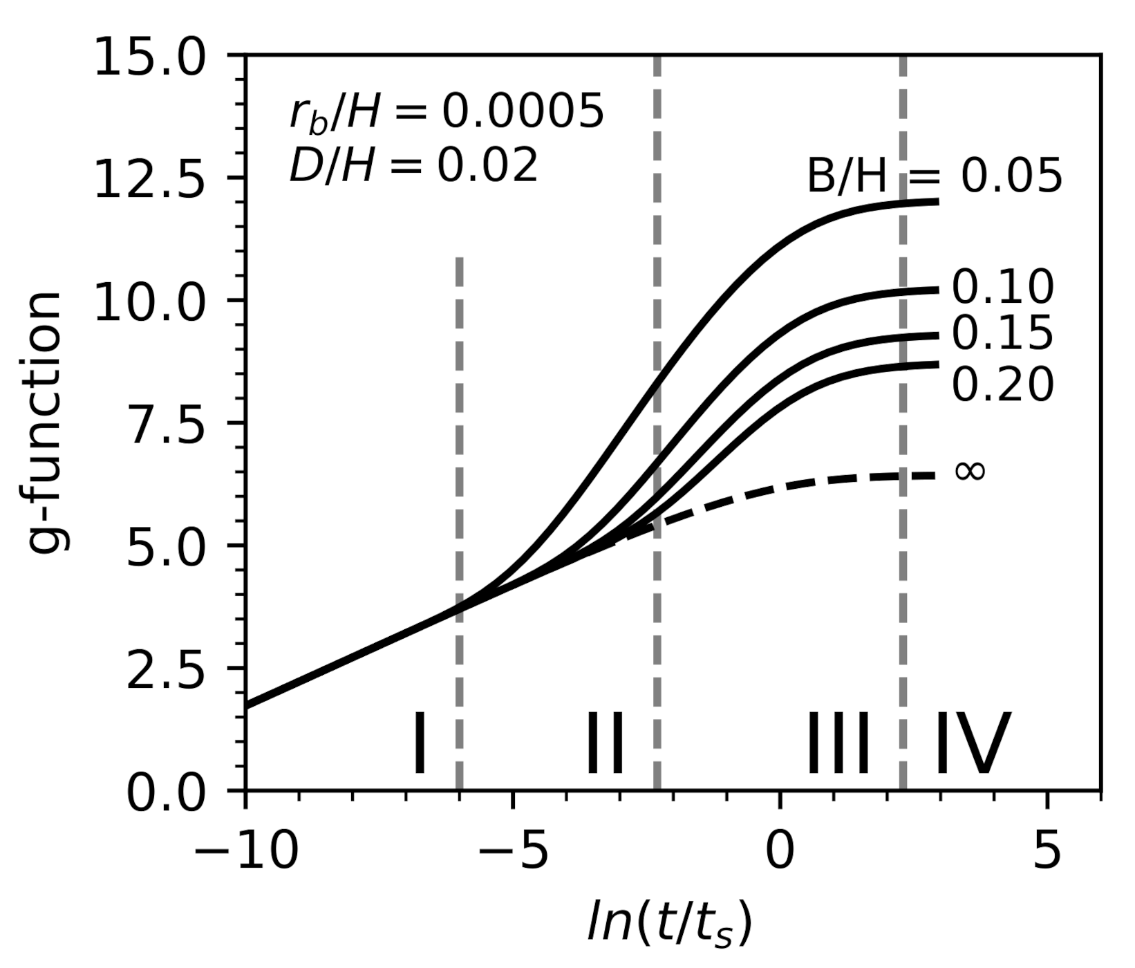
Figure 1. g-functions for a 2 by 2 borefield. Region I: radial 1D heat transfer dominates the heat transfer process. Region II: heat transfer is affected by the thermal interaction between boreholes. Region III: axial 2D heat transfer effects influence the heat transfer process. Region IV: steady-state region.
Energies 13 06203 g001
Figure 2. The shadow cost concept.
Energies 13 06203 g002
Figure 3. Graphical representation of Equation (10), with the vector of aggregated loads evaluated at k = N S T .
Energies 13 06203 g003
Figure 4. Schematic of the validation case study. The optimization variables are the ground-source heat pumps (GSHP) modulation signal ( u 1 ), the regeneration heat exchanger circulation pump ( u 2 ), the auxiliary electric heater signal ( u 3 ) .
Energies 13 06203 g004
Figure 5. Behavior of the daily average of control input variables for the different strategies in year 10. The background color indicates the different seasons: autumn (yellow), winter (blue), spring (green) and summer (red).
Energies 13 06203 g005
Figure 6. Comparison of the regeneration heat exchanger variables for strategies 2 and 3 during the last year summer season. From top to bottom: inlet temperatures at the borefield side, heat capacity rates, heat exchanger effectiveness and heat exchanger actual/maximum heat flow.
Energies 13 06203 g006
Figure 7. Yearly share of the thermal energy supplied to the building by the GSHP and the auxiliary heater for the different strategies over the 10 years period.
Energies 13 06203 g007
Figure 8. Yearly distribution of operational costs (left-axis, bar plot) and accumulated operational costs (right-axis, line plot) for the different strategies (S1-first bar, S2-second bar and S3-third bar) over the 10 years period.
Energies 13 06203 g008
Figure 9. Comparison of different long-term horizons length and resolution during last year summer season. Top: regeneration pump input signal. Bottom: total predicted heat supplied and its share over the GSHP and auxiliary heater for the forecasted long-term horizon.
Energies 13 06203 g009
Figure 10. Comparison of the first weekly predictions and the actual values from the simulation. From top to bottom: GSHP condenser energy, auxiliary energy, regenerated energy, SCOP and average fluid temperature. From left to right: Strategy 3, 3d and 3e.
Energies 13 06203 g010
Figure 11. Comparison of the first monthly predictions and the actual values from the simulation. From top to bottom: GSHP condenser energy, auxiliary energy, regenerated energy, seasonal coefficient of performance (SCOP) and average fluid temperature. From left to right: Strategy 3, 3d and 3e.
Energies 13 06203 g011
Table 1. Summary of the building envelope parameters. The layers are ordered from inside to outside.
Elementk [W/mK]t [m]U [W/m 2 K] ρ [kg/m 3 ] c p [J/kgK]
Outer wall
Concrete block0.510.202.5514001000
Foam insulation0.040.170.235101400
Wood siding0.140.0114.0530900
Total 0.195
Floor
Concrete slab1.130.0814.1314001000
Insulation0.040.200.21010
Concrete slab1.130.353.2314001000
Total 0.123
Roof
Plasterboard0.160.0116.0950840
Concrete slab1.130.0814.1314001000
Fibreglass quilt0.040.150.26612840
Roofdeck0.140.027.0430900
Total 0.184
Windows:U-value:1.0 W/m 2 K g-factor:0.598
Table 2. Heat pump fit coefficients used in Equations (13) and (20).
123
A23,152522.3−51.7
B17,138522.0−170.5
C−34.590.1380.0071
Table 3. Summary of the borefield parameters of the building.
Borehole ParametersPiping Parameters
NotationDescriptionValueUnitNotationDescriptionValueUnit
r b o r Borehole radius75.0mm r p Pipe radius20.0mm
H b o r Borehole height125.0m k p Pipe conductivity0.5W/(mK)
d b o r Borehole burial depth0m t p Pipe thickness2.0mm
n b o r Number of boreholes4- x p Pipe spacing80.0mm
Ground ParametersGrout Parameters
NotationDescriptionValueUnitNotationDescriptionValueUnit
k s Ground conductivity2.0W/(mK) k g Grout conductivity1.15W/(mK)
c s Ground heat capacity1200J/(kgK) c g Grout heat capacity800J/(kgK)
ρ s Ground density1800kg/m 3 ρ g Grout density1600kg/m 3
T s Undisturbed ground temperature10 C
d T s / d z Geothermal gradient0.01 C/m
Table 4. HVAC equipment parameters.
NotationDescriptionValueUnit
Q ˙ c o n , n o m GSHP nominal capacity26kW
Q ˙ a u x , n o m Auxiliary system nominal power40kW
U A Heat exchanger heat transfer coefficient10,000W/K
Δ p n o m Pump nominal pressure drop120kPa
m ˙ n o m Pump nominal mass flow rate1.6kg/s
W ˙ p u m , n o m Pump nominal power400W
Table 5. Prediction horizons considered for the Model Predictive Control (MPC) and shadow cost.
Interval No.1234567891011121314
MPC (N ST )
Interval size1 h1 h1 h1 h2 h2 h4 h4 h8 h12 h12 h24 h48 h48 h
Time elapsed1 h2 h3 h4 h6 h8 h12 h16 h1 d1.5 d2 d3 d5 d7 d
Shadow cost (N LT )
Interval size1 w1 w1 w1 m1 m1 m1 m1 m1 m1 m1 m1 m1 m1 m
Time elapsed2 w3 w1 m2 m3 m4 m5 m6 m7 m8 m9 m10 m11 m12 m
Table 6. Comparison of control strategies 1, 2 and 3 over 10 years.
Strategy 1:Strategy 2:Strategy 3:
Key Performance IndicatorUnitMPCMPC + RBCMPC + Shadow Cost
GSHP condenser energy useMWh380.01401.18398.85
GSHP compressor energy useMWh70.2773.8973.20
SCOP5.415.435.45
Auxiliary (thermal) energy useMWh93.0172.2373.29
Regeneration pump energy useMWh~08.881.00
Regenerated energyMWh0.28148.85137.45
Total operational costs$33,30931,62330,090
Average number of iterations48.1949.3672.95
Average time per iterations0.01150.00880.0311
Table 7. Long-term horizons considered for the shadow costs in strategies 3, 3b and 3c.
Interval No.1234567891011121314
Strategy 3
Interval size1 w1 w1 w1 m1 m1 m1 m1 m1 m1 m1 m1 m1 m1m
Time elapsed2 w3 w1 m2 m3 m4 m5 m6 m7 m8 m9 m10 m11 m12 m
Strategy 3b
Interval size1 w1 w1 w1 w1 w1 w1 w1 w1 w1 w1 w1 m1 m1 m
Time elapsed2 w3 w4 w5 w6 w7 w8 w9 w10 w11 w3 m4 m5 m6 m
Strategy 3c
Interval size1 w1 w1 w1 m1 m1 m1 m1 m
Time elapsed2 w3 w1 m2 m3 m4 m5 m6 m
Table 8. Comparison of long-term control strategies 3, 3b and 3c over 10 years.
Key Performance IndicatorUnitStrategy 3Strategy 3bStrategy 3c
GSHP condenser energy useMWh398.85398.65398.21
GSHP compressor energy useMWh73.2073.2473.13
SCOP5.455.455.45
Auxiliary (thermal) energy useMWh73.2974.1874.43
Regeneration pump energy useMWh1.000.690.66
Regenerated energyMWh137.45130.69129.48
Total operational costs$30,09030,21430,239
Average number of iterations72.9572.8261.01
Average time per iterations0.03110.03120.0268
Table 9. Comparison of long-term control strategies 3, 3d and 3e over 10 years.
Key Performance IndicatorUnitStrategy 3Strategy 3dStrategy 3e
GSHP condenser energy useMWh398.85398.24397.45
GSHP compressor useMWh73.2073.1073.08
SCOP5.455.455.45
Auxiliary (thermal) energy useMWh73.2973.5475.26
Regeneration pump energy useMWh1.001.060.26
Regenerated energyMWh137.45137.85118.28
Total operational costs$30,09030,13230,316
Average number of iterations72.9573.6474.76
Average time per iterations0.03110.03140.0329
Publisher’s Note: MDPI stays neutral with regard to jurisdictional claims in published maps and institutional affiliations.