True Amplitude Angle Gathers from Reverse Time Migration by Wavefield Decomposition at Excitation Amplitude Time

Abstract

Reservoir parameter estimation is one of the goals of amplitude-versus-angle (AVA) inversion and angle-domain common image gathers are the basis of AVA inversion. Therefore, the accuracy of kinematic and kinetic information on angle gathers is very important for reservoir characterization. Reverse time migration is one of the most physically accurate migration method. Generating angle gathers from reverse time migration with the Poynting vector method is very efficient. However, due to inaccurate angle measurement and uneven illumination, angle gathers calculated by the Poynting vector method are often not suitable for AVA inversion. In this paper, we propose an efficient method of angle gathers with accurate angular information and amplitude from reverse time migration. We firstly decompose source and receiver wavefield to their up-going and down-going parts by using analytic wavefield. We calculate propagation directions for source down-going wavefield and receiver up-going wavefield by the Poynting vector method and form the angle gathers with these angle information and decomposed wavefield. To reduce memory storage and improve computational efficiency, we decompose wavefield at excitation amplitude time by using a local spatial Fourier transform. We also use a spatial smoothed Poynting vector to improve the stability of angle measurement. We apply an illumination compensation image condition to recover the true amplitude. Numerical examples on Marmousi model and the SEAM two-dimensional (2D) model demonstrate the advantages of our proposed method. The angle gathers based on our method are cleaner with more focus on events energy and better continuity, suffering from less low-frequency noise in the shallow parts and with a distinct cutoff at large angle where reflection terminates. At last, we demonstrate the effectiveness of proposed method on a 2D marine field data example.

1. Introduction

The technology of amplitude versus angle (AVA) has been widely used to estimate subsurface petrophysical properties and predict fluid in the reservoirs for decades [1,2,3]. The input data for AVA analysis are angle gathers which are generated during the seismic migration process. Traditional approaches of calculating angle gathers are commonly implemented in ray-based migration methods since the ray-based propagator naturally provides angle information. However, the ray-based methods are limited by the high-frequency asymptotic approximation [4,5], thus, the wave equation based methods [6] were adopted for the angle gathers calculation.

As the wave equation-based methods do not provide propagation direction explicitly, several methods were proposed to extract angle information from wavefield. These methods can be summarized into two main categories. The first group applies the integral method, e.g., the local-plane wave decomposition and wavelet transform based methods [7,8,9], local Fourier transform based methods [10,11]. The second group applies differential methods, e.g., the Poynting vector or gradient vector-based methods [12,13,14,15,16]. Since the differential type methods only need to calculate spatial and temporal derivatives at specified locations, these methods are very efficient and easy to implement. Instead, the integral type methods need to analyze the local wavefield within a neighboring area, and these methods involve more computations, which are more time-consuming. However, compared to the differential methods, the integral methods are more stable, reliable and can handle the case of multi-arrivals.

To improve the accuracy and reliability of the differential methods, several methods were proposed, such as, stabilizing angle measurement in the time window [17], using time-shift Poynting vectors [18], smoothing the Poynting vectors in the space domain [13], using a least squares solution over the time or space [14], using the optical flow method to stabilize Poynting vector directions [19,20,21], using the traveltime gradient of first arrival to calculate the source-side wave propagation direction [22,23], or calculating angle just at most energetic arrival [16]. All these methods are effective to improve accuracy, and cannot deal with the situation of multiarrivals and overlapping events. Poynting vector methods were also applied to seismic illumination and resolution analyses, which can be used to correct the migration image [16]. The amplitude of angle gathers can be preserved by source illumination [24].

In this paper, we propose a new method to generate angle gathers under the reverse time migration frame, in which the angle information is calculated by a hybrid method. We first construct analytic wavefield and then decompose them into up-going and down-going parts in time-wavenumber domain. Then, we use the spatial weighted Poynting vectors method to calculate the wave propagation angle and obtain angle gathers with an angle domain illumination compensation imaging condition. Finally, we compare the angle gathers extracted by different methods and validate our method in the Marmousi model and 2D SEAM model to clarify the superiority of the proposed method.

2. Methods

2.1. Wavefield Decomposition in t–k Domain

Extracting the angle information by using the differential type methods (e.g., Poynting vectors) is highly efficient. However, these methods can only give one direction per spatial grid point, which means that if there are more than one wavefront coexists at one space point at the same time, the correct direction cannot be estimated with these methods. The overlapping of wavefield mainly occurs in two situations, the first situation is that the incident wave, reflected wave and transmitted wave coexist on the reflector, and the second one refers to that the multipath wavefield overlap at the same time. The former has great influence on the angle gathers, because it occurs on every reflector that needs to be imaged.

In order to deal with the overlapping wavefield at the reflector, we can separate source and receiver wavefield into their up-going, and down-going parts, respectively,

$$s(t,x)=s_u(t,x)+s_d(t,x)$$

(1)

$$r(t,x)=r_u(t,x)+r_d(t,x)$$

(2)

where $s(t,x)$, $r(t,x)$ are source wavefield and receiver wavefield respectively. $s_{u,d}(t,x)$ are source up- and down-going parts respectively. $r_{u,d}(t,x)$ are receiver up- and down-going parts respectively. And $x=(x,z)$, namely, $s(t,x)=s(t,x,z)$ and $r(t,x)=r(t,x,z)$. The conventional procedure to obtain the wave components in Equations (1) and (2) can be illustrated as follows [25]:

$$S_U(\omega ,k_z)=\{\begin{array}{c}S(\omega ,k_z)\hspace{0.17em}\hspace{0.17em}\hspace{0.17em}\omega k_z>0\\ 0\hspace{0.17em}\hspace{0.17em}\hspace{0.17em}\hspace{0.17em}\hspace{0.17em}\hspace{0.17em}\hspace{0.17em}\hspace{0.17em}\hspace{0.17em}\hspace{0.17em}\hspace{0.17em}\hspace{0.17em}\hspace{0.17em}\omega k_z\le 0\end{array}$$

(3)

$$S_D(\omega ,k_z)=\{\begin{array}{c}0\hspace{0.17em}\hspace{0.17em}\hspace{0.17em}\hspace{0.17em}\hspace{0.17em}\hspace{0.17em}\hspace{0.17em}\hspace{0.17em}\hspace{0.17em}\hspace{0.17em}\hspace{0.17em}\hspace{0.17em}\hspace{0.17em}\omega k_z\ge 0\\ S(\omega ,k_z)\hspace{0.17em}\hspace{0.17em}\hspace{0.17em}\omega k_z<0\end{array}$$

(4)

where $S(\omega ,k_z)$ is two-directional (2D) Fourier transform of $s(t,z)$, $\omega$ is the angular frequency, $k_z$ is the vertical wavenumber, $S_U(\omega ,k_z)$ and $S_D(\omega ,k_z)$ are source up/down going wavefield in $\omega -k_z$ domain respectively, likewise as receiver wavefield. The conventional method requires both signs of frequency and wavenumber to determine the up-going or down-going directions. Therefore, we need to store the entire wavefield, because the frequency information is obtained by performing Fourier transform on time axis, which is the slowest dimension of time-domain RTM. In order to reduce I/O cost, with the help of the characteristic that the analytic signal only has positive frequency components, we can construct analytic wavefield at first, and then decompose the analytic wavefield into up-going and down-going components through on-directional (1D) Fourier transform [26],

$$\widehat{S}(t,x)=s(t,x)+i\cdot H[s(t,x)]$$

(5)

$${\widehat{S}}_U(t,k_z)=\{\begin{array}{c}\widehat{S}(t,k_z)\hspace{0.17em}\hspace{0.17em}\hspace{0.17em}{k}_z>0\\ 0\hspace{0.17em}\hspace{0.17em}\hspace{0.17em}\hspace{0.17em}\hspace{0.17em}\hspace{0.17em}\hspace{0.17em}\hspace{0.17em}\hspace{0.17em}\hspace{0.17em}\hspace{0.17em}{k}_z\le 0\end{array}$$

(6)

$${\widehat{S}}_D(t,k_z)=\{\begin{array}{l}\widehat{S}(t,k_z)\hspace{0.17em}\hspace{0.17em}\hspace{0.17em}{k}_z<0\\ 0\hspace{0.17em}\hspace{0.17em}\hspace{0.17em}\hspace{0.17em}\hspace{0.17em}\hspace{0.17em}\hspace{0.17em}\hspace{0.17em}\hspace{0.17em}\hspace{0.17em}\hspace{0.17em}{k}_z\ge 0\end{array}$$

(7)

$$s_{u,d}(t,x)=\mathrm{Re}\left[F^{-1}[{\widehat{S}}_{U,D}(t,k_z)]\right]$$

(8)

where $\widehat{S}(t,k_z)\hspace{0.17em}$ is 1D Fourier transform of the analytic source wavefield $\widehat{S}(t,x)$, and $k_z$ is vertical wavenumber. ${\widehat{S}}_{U,D}(t,k_z)$ and $s_{u,d}(t,x)$ are source up/down-going components in time-wavenumber domain, and time-space domain, respectively. $H[\cdot ]$ is Hilbert transform, $F^{-1}[\cdot ]$ is 1D inverse Fourier Transform. $Re[\cdot ]$ operator takes out the real part of analytic wavefield. Likewise as receiver side wavefield.

In order to avoid the convolution along the time axis of the Hilbert transform, we can apply the Hilbert transform to the source term and solve the wave equation to get the imaginary part of analytic wavefield [27]. However, decomposing wavefield by Fourier transform at each time step during wave extrapolation is very time-consuming especially in 3D case. Therefore, we just decompose wavefield in a local spatial window at excitation amplitude time [28,29] and separate wavefield into local angle components by weighted Poynting vectors [13]. The excitation time can be calculated by two methods: Ray tracing [30] and measuring the maximum amplitude of source wavefield [28,29]. We applied the second method, whereby the most energetic arrival time is used. We scan the source wavefield twice, first scan to locate the arrival time of most energetic amplitude, then decompose wavefield in the second scan. The twice-scanning procedure does not need additional computation since the source wavefield needs to be stored reproduced to correlate with receiver wavefield in RTM imaging.

2.2. Imaging in Angle Domain

Zero-lag cross correlation imaging condition can obtain RTM image stably. However, the resulting image does not have any physical meaning since the amplitude is unrelated to reflectivity. Deconvolution imaging condition can provide images related to reflectivity but becomes unstable when the denominator is small. In order to obtain stable angle gathers related to angle-dependent reflection coefficients, we apply a source-normalized imaging condition. The local angle image for an image location x can be obtained by,

$$I(x,{\theta }_s,{\theta }_g)=\frac{{\displaystyle \int s_d(x,{\theta }_s,t)\cdot r_u(x,{\theta }_g,t)dt}}{{\displaystyle \int s_d^2(x,{\theta }_s,t)dt}}$$

(9)

where $s_d(x,{\theta }_s,t)$ is the angle component of source-side down-going wavefield and $r_u(x,{\theta }_g,t)$ is the angle component of receiver-side up-going wavefield. ${\theta }_s$ and ${\theta }_g$ are local incident angle and local scattering angle respectively. We can convert the local angle image from (${\theta }_s$,${\theta }_g$) domain to (${\theta }_r$,${\theta }_d$) domain by a coordinate transform,

$${\theta }_d=({\theta }_s+{\theta }_g)/2$$

(10)

and

$${\theta }_r=({\theta }_s-{\theta }_g)/2$$

(11)

where ${\theta }_r$ is the reflection angle and ${\theta }_d$ is the target dipping angle. Since the AVA response is reflection-angle-dependent, the angle gathers can be obtained from a local angle image:

$$I(x,{\theta }_r)={\displaystyle \sum _{{\theta }_d}I(x,{\theta }_r,{\theta }_d)}.$$

(12)

3. Results

3.1. Angle Mesurement Analysis

We design a simple two layer model which is shown in Figure 1a to compare different angle measurement methods. We calculate angle gathers of one point (x = 3 km) with one shot (x = 2.4 km) by using different angle measurement methods. As mentioned above, the coexistence of incident wave, reflected wave and transmitted wave on the reflector will lead to the inaccurate angle measurement. In order to evaluate the influence of this situation on the angle measurement, we introduce a constant velocity model (Figure 1b) as migration velocity model which does not produce reflections. We use four methods to analyze the angle measurement, which are Poynting vector method, weighted Poynting vectors method, optical flow method and proposed method (wavefield decomposition plus weighted Poynting vectors). For simplicity, these four methods are referred to as Method 1, to Method 4, respectively.

At first, we use the constant velocity model as migration velocity, and the angle gathers calculated by four methods are shown in Figure 2. Given there is a flat reflector at 1 km depth, the theoretical reflection angle is about 31° marked by the black solid line. As there is no interference of reflected wave, accurate reflection angle can be obtained with all these four methods. However, there are some smearing artifacts caused by unstable angle measurement in Figure 2a, which is the disadvantage of Poynting vector method [31]. The similar accuracy can be achieved by the other three methods in constant velocity model.

Then, we use the true model as migration velocity to extract angle gathers at 3 km. Figure 3a–d are the angle gathers calculated by Method 1, to 4, respectively. From Figure 3a–d, we can see that the reflection angle calculated by Method 1 deviates the most from the true value, while the angle calculated by Method 4 is closest to the theoretical angle. Smearing artifacts and backscattering noises can be effectively eliminated with Method 4.

Furthermore, we use true velocity model to generate the multi-shot angle gathers by using these four methods. The acquisition system is composed of 13 shots from 2.4 km to 3 km with a source interval of 50 m, and the angle gathers are extracted at 3 km, in which the theoretical reflection angle is about 0~31°. Figure 4a,b are the angle gathers calculated by Method 1 to 4. As illustrated in these figures, the angle gathers calculated by the first three methods are affected by smearing artifacts and low frequency noises (indicated by the red dashed box), while relatively accurate angle and sharp cutoff, at the end of reflection, can be obtained with Method 4. Moreover, smearing artifacts and low frequency noises can be efficiently eliminated by using Method 4.

3.2. Numerical Examples

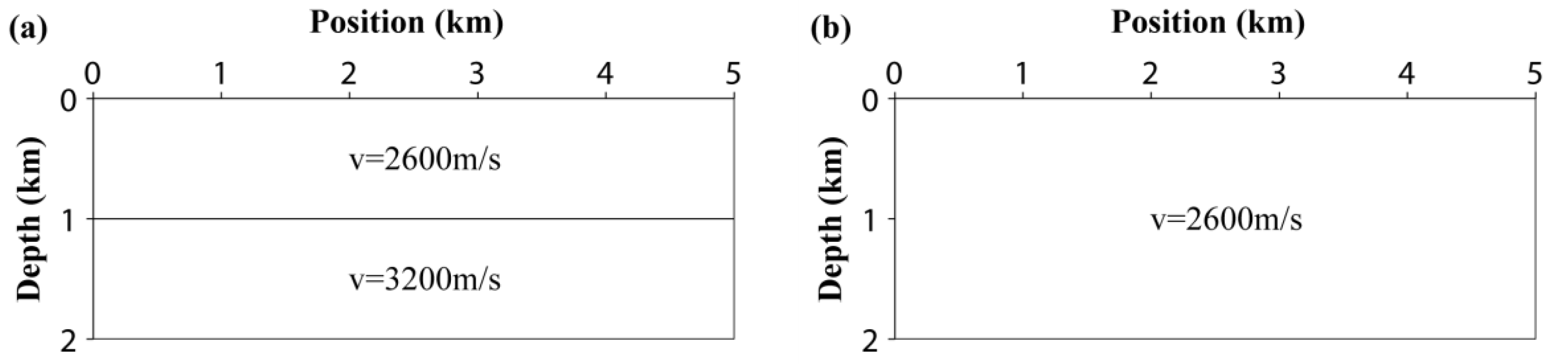
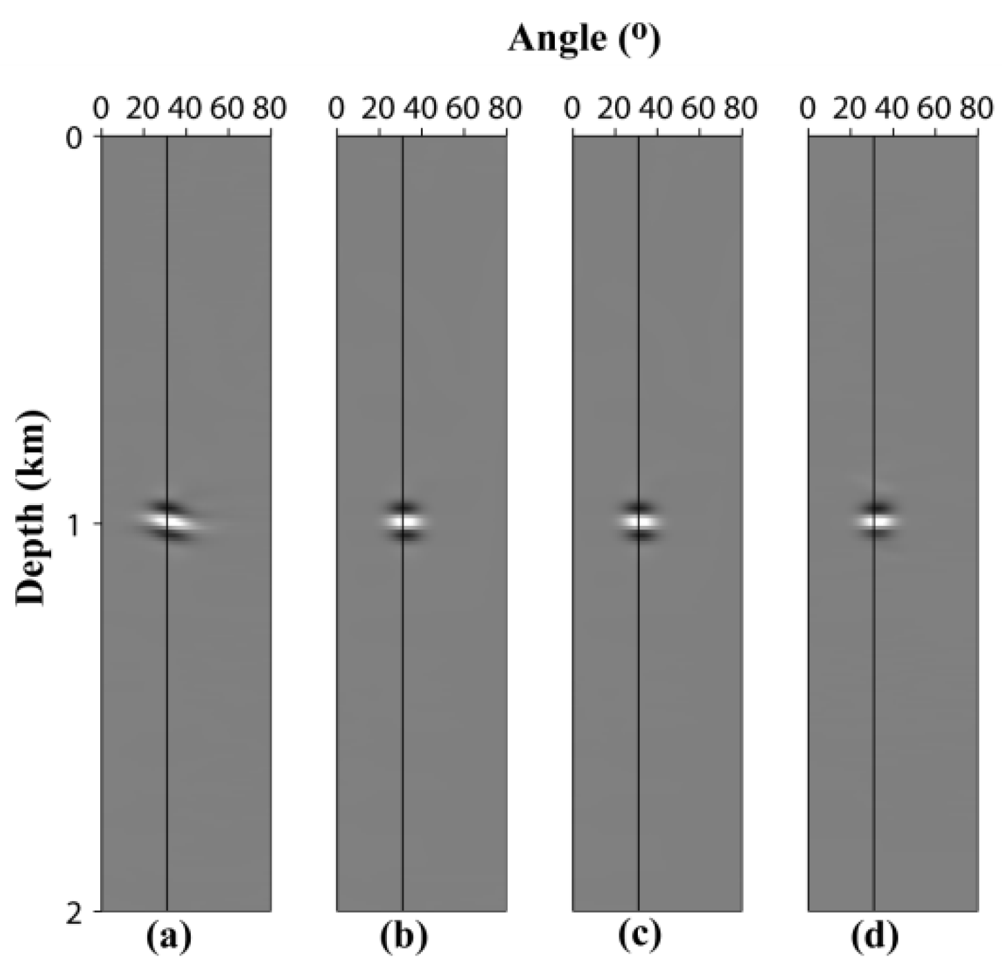
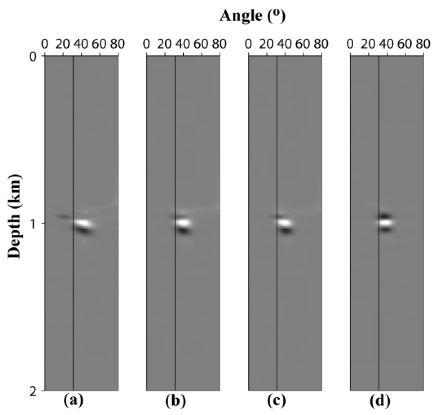
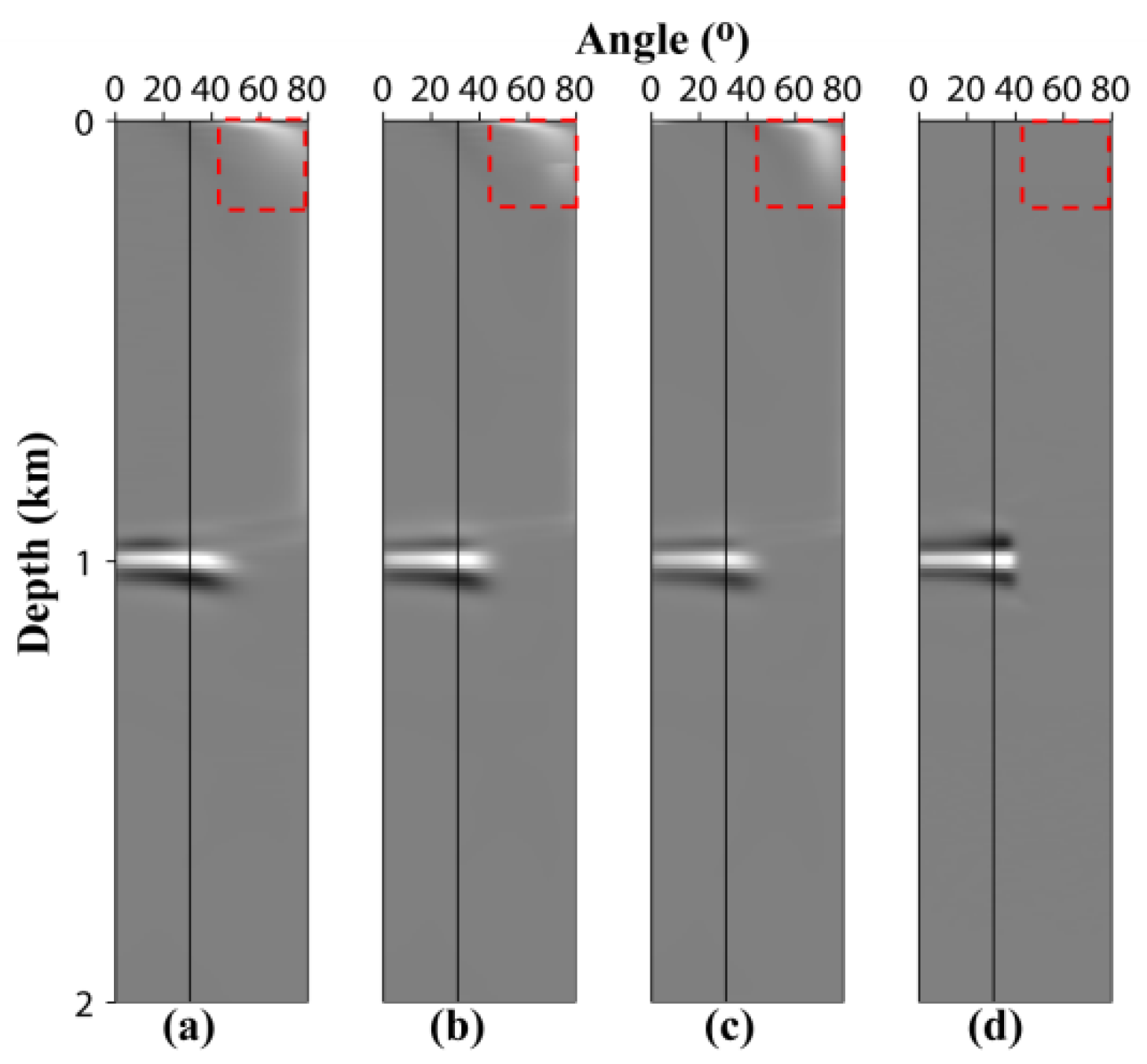
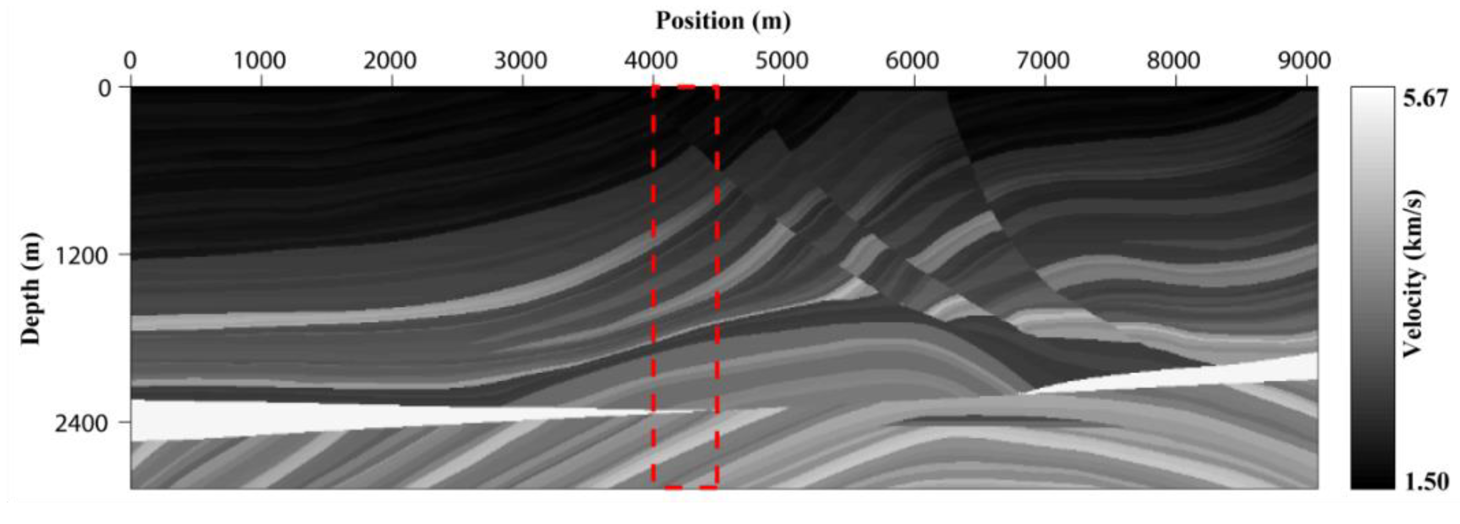
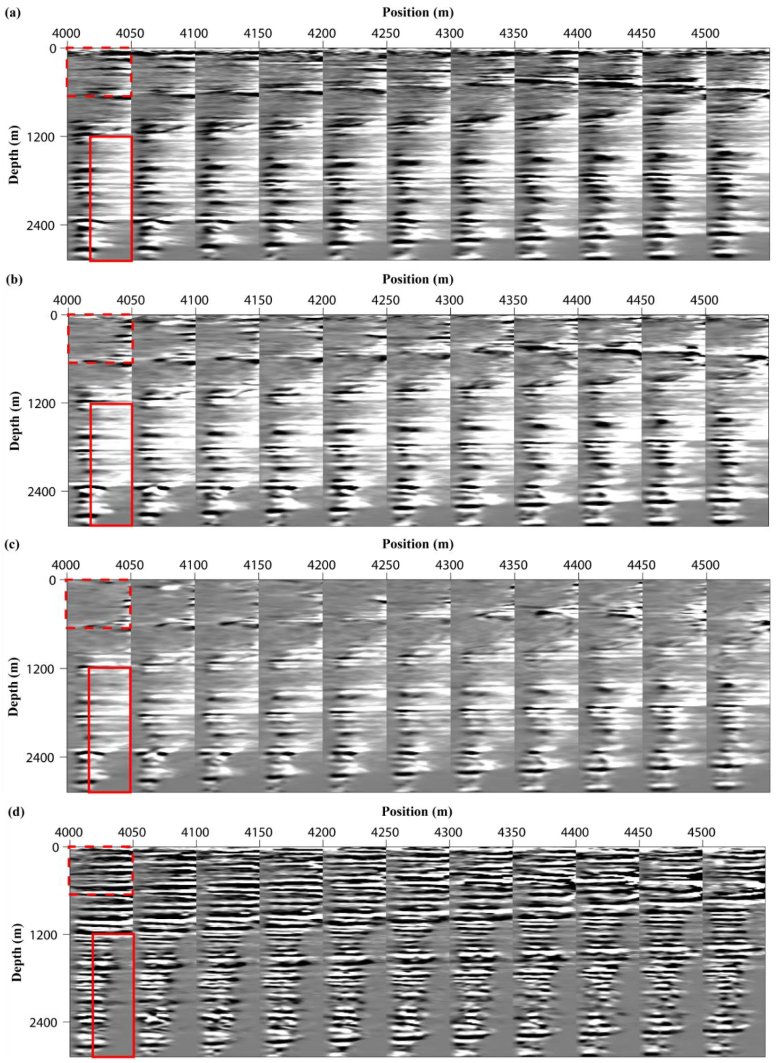
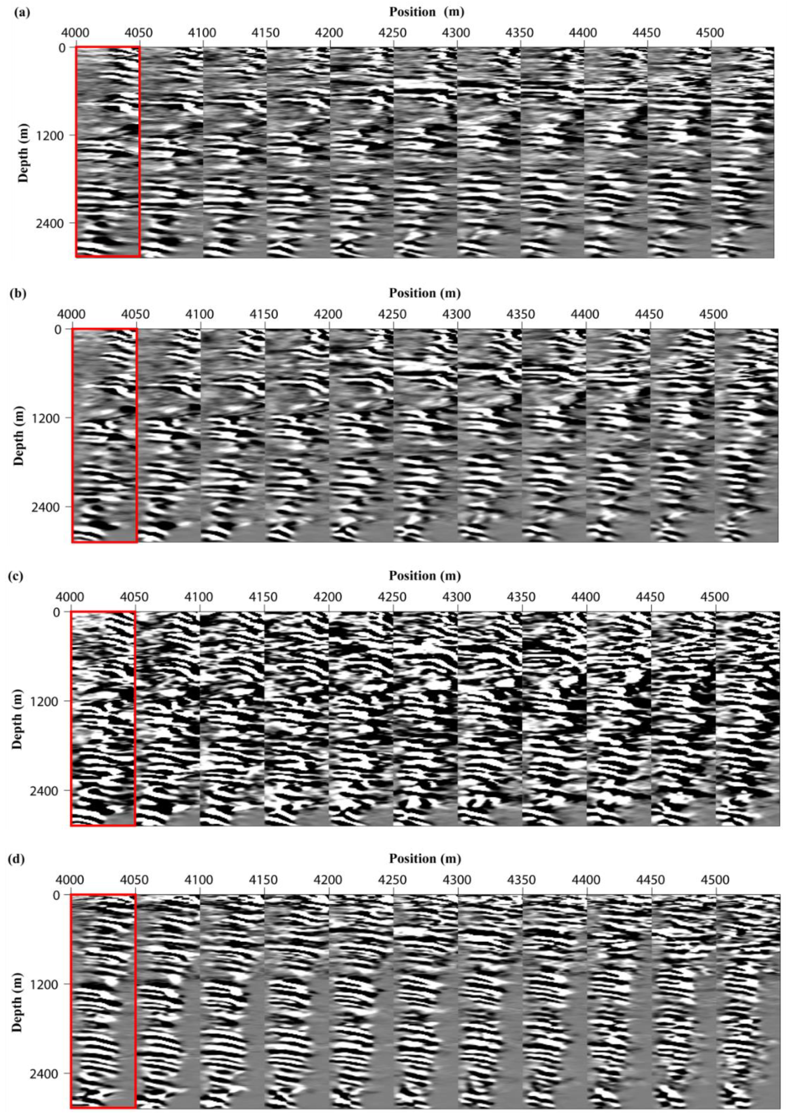
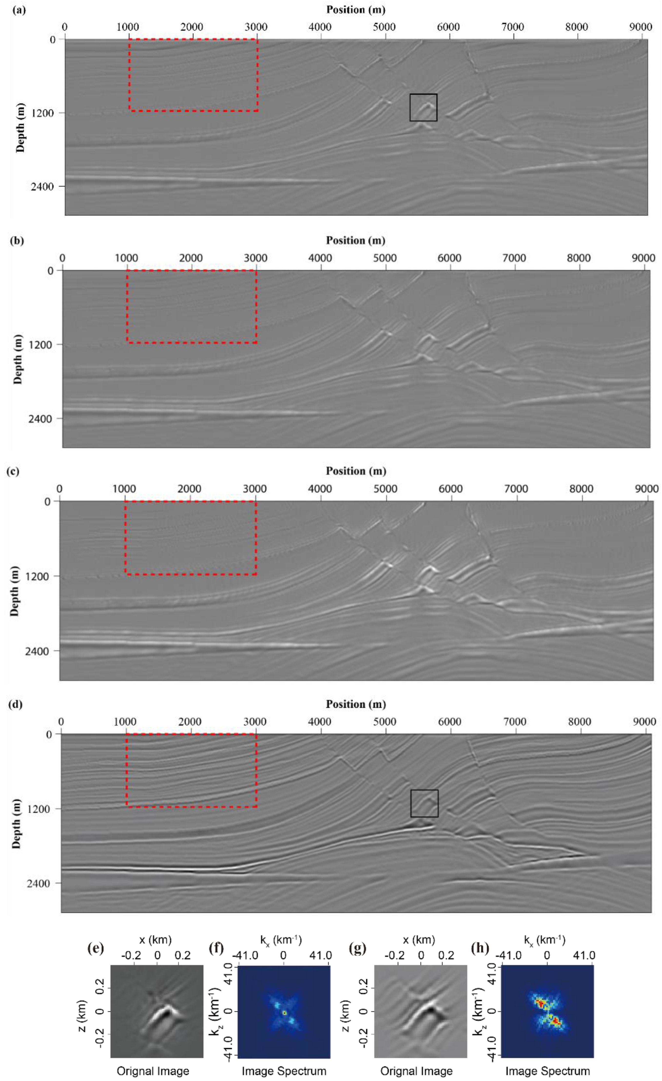
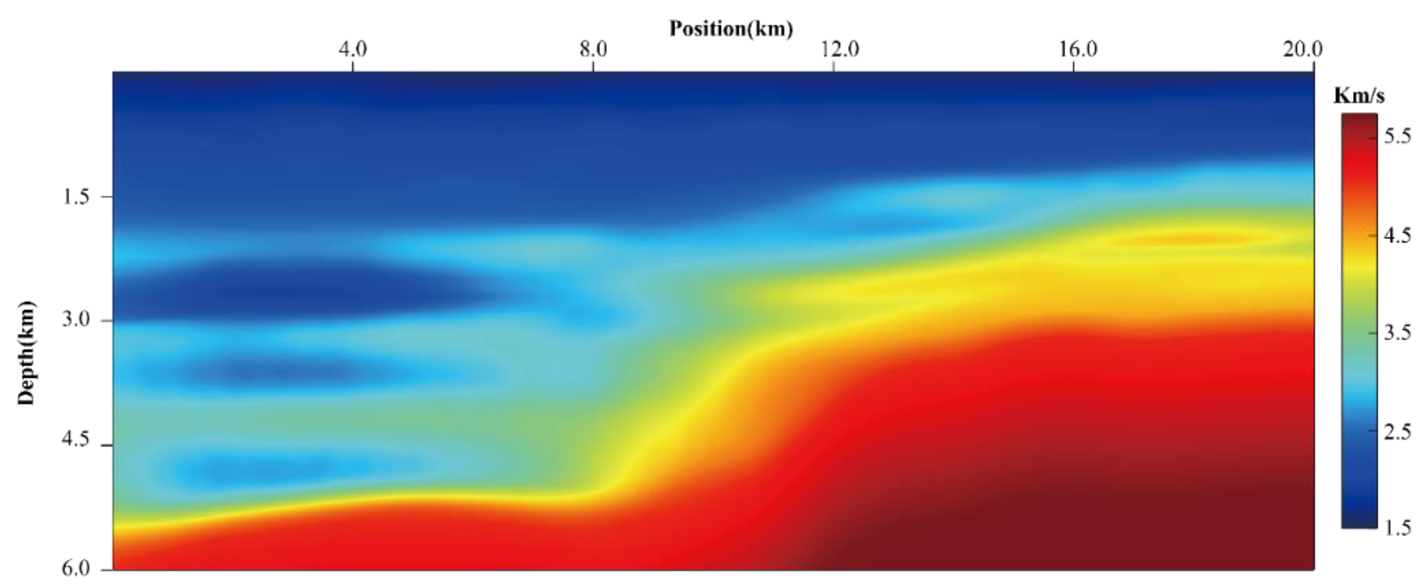
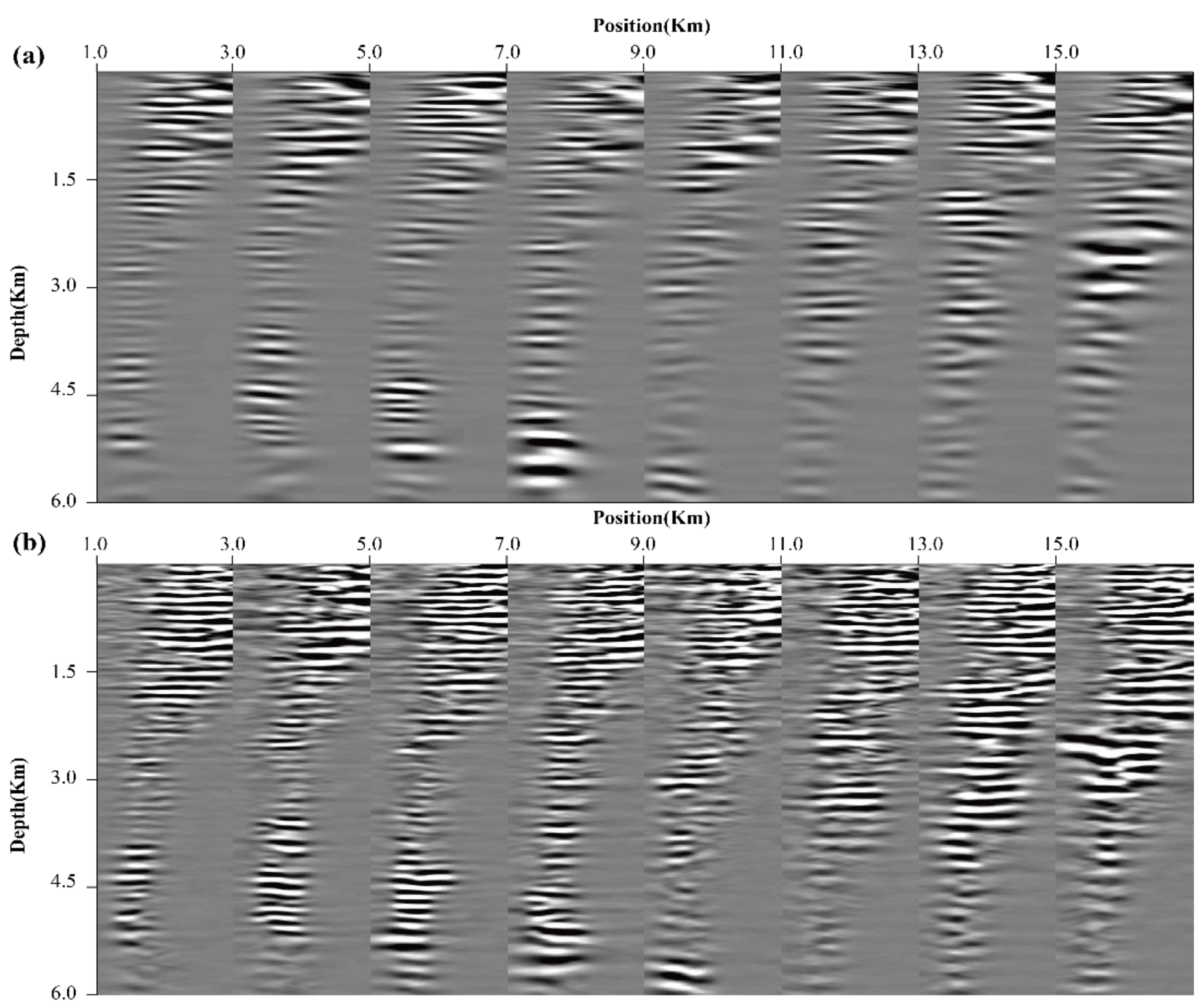
3.2.1. Marmousi Model

In the first example, we extract angle gathers on the Marmousi model. The acquisition system is composed of 225 shots with a source interval of 50 m, and there are 200 receivers on the left side in each shot. The minimum and maximum offsets are 0 and 4975 m and the receiver interval is 25 m. Both the horizontal and vertical grid intervals are 12.5 m. The time interval is 1 ms. The source is a 20 Hz Ricker wavelet. In order to compare the effects of different methods, we first calculate the angle gathers, using four methods, based on the true velocity model. Partial results (indicated by the red dashed rectangle in Figure 5) are shown in Figure 6. Then, we use an incorrect velocity model as the migration velocity model to compute the angle gathers which are shown in Figure 7. As illustrated in Figure 6a–c, the angle gathers are very noisy and the events energy are not concentrated due to the inaccurate angle measurement. Methods 1 to 3 cannot handle with back-scattering artifacts if there are complex structures. On the contrary, the angle gathers in Figure 6d are with higher signal-to-noise ratio and clear cutoff at large angle which is shown in the red solid rectangles. Moreover, the shallow reflector marked in red dashed box can be clearly imaged in Figure 6d, while the obvious events cannot be obtained by the first three methods, especially at small angles.

In Figure 7, due to the incorrect migration velocity model, most of the source wavefields and receiver wavefields are not in the same wavepath. Therefore, there are fewer back-scattering artifacts in Figure 7a–c than in Figure 6a–c. The angle gathers in Figure 7d are with the best quality among the four results. In details, the angle gathers in Figure 7d are cleaner, more concentrated, with better continuity and sharper cutoff. It is also shown that the angle gathers calculated by Method 4 are more suitable for the migration velocity analysis because the curvatures are easier to pick up.

In Figure 8, we generate the stack images with the reflection angle from 0 to 50° of four methods. Since large reflection angles are excluded, all images do not suffer from low-frequency noise. Compared with Figure 8a–c, the stack image by Method 4 in Figure 8d is with consistent layered structures in the shallow part marked by red dash rectangles, more balanced amplitudes, and sharper images in general. The areas marked by black square in Figure 8a,d are chosen to quantitatively compare the resolution of stack images. Figure 8e,f are the local image and wavenumber spectrum of stack image by Method 1, Figure 8g,h are the local image and wavenumber spectrum of stack image by Method 4. In Figure 8f, the energy is mainly concentrated on the low wavenumber part since the reflection angle is incorrectly estimated. After accurate angle calculation by Method 4, the energy distribution on the wavenumber spectrum is more balanced which can be shown in Figure 8h.

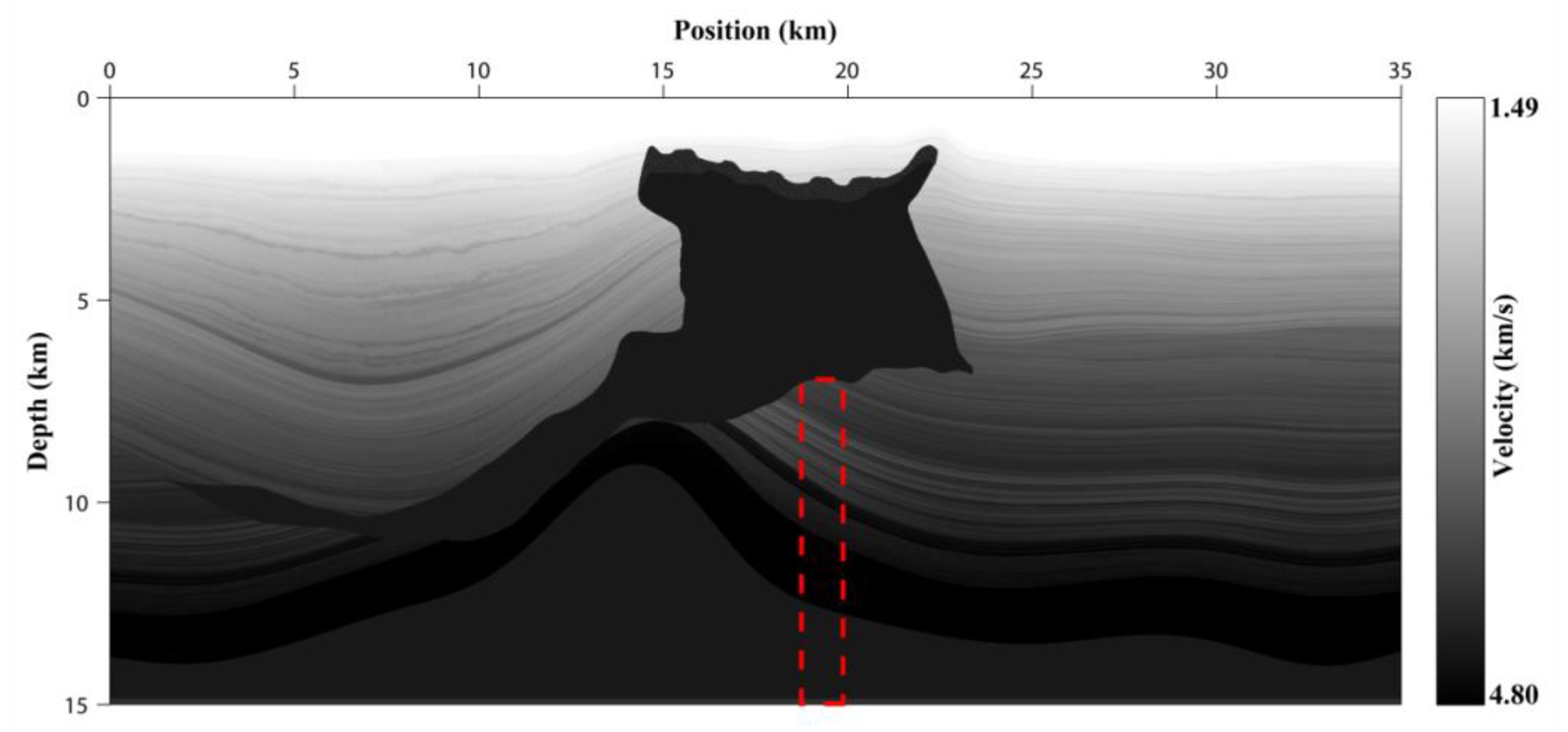
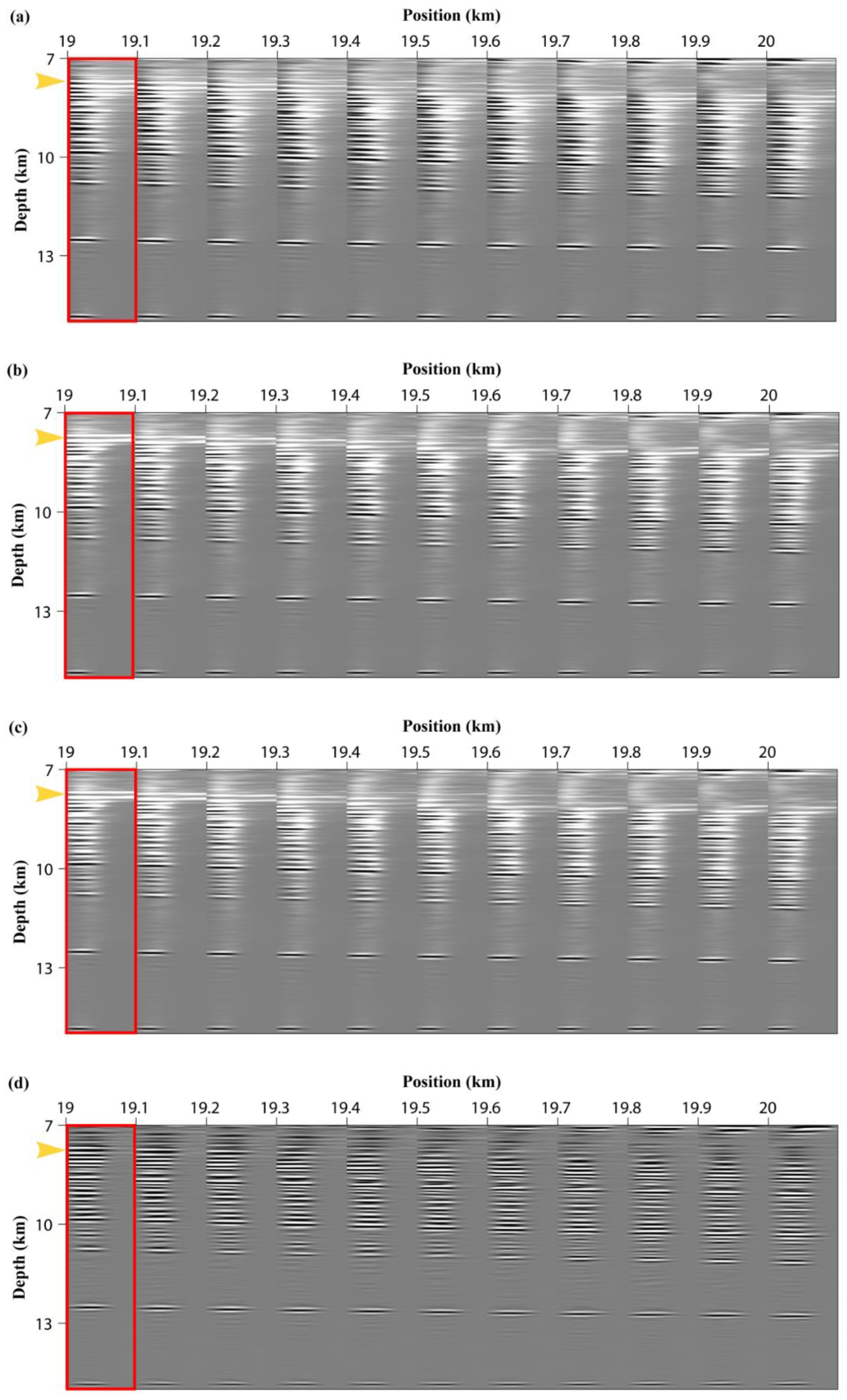
3.2.2. SEAM 2D Model

In order to evaluate the quality of subsalt imaging, we investigated a 2D section of the SEAM phase I model in this example. The P wave velocity model is shown in Figure 9. The acquisition system is composed of 400 shots with a source interval of 80 m. The minimum and maximum offsets are 0 and 7980 m and the receiver interval is 40 m. The horizontal and vertical grid intervals are 20 m, and 10 m, respectively. The time interval is 1 ms. The source is a 20 Hz Ricker wavelet.

We selected a subsalt area marked by red dashed rectangles in Figure 9 to demonstrate the angle gathers. The results are shown in Figure 10. The angle gathers that were calculated by Method 2 (Figure 10b) and Method 3 (Figure 10c) have a sharper cutoff at the large reflection angle than the angle gathers calculated by Method 1 (Figure 10a) because weighted Poynting vector and optical flow can stabilize the angle measurement. Nevertheless, these three methods do not separate the up-going and down-going wavefield, so the artifacts and low-frequency noises caused by backscattering wave cannot be effectively eliminated, and the errors of angle measurement still exist. By contrast, Method 4 decomposes wavefield into up-going and down-going parts, and is effective in eliminating the influence of multiarrivals and obtains more accurate angle measurement. As a result, angle gathers in Figure 10d are with higher signal-to-noise ratio, more balanced amplitude, and wider angle coverage.

3.2.3. Field Data

Finally, we test our method with a 2D marine field data. Figure 11 shows the migration velocity model. The acquisition system is composed of 530 shots with a source interval of 50 m, and there are 360 receivers on the left side in each shot and the receiver interval is 12.5 m. The minimum and maximum offsets are 183 and 4670.5 m. We generated the angles using Method 1 and Method 4 shown in Figure 12a,b. We can see that the angle gathers calculated by Method 4 are more energy-balanced and continuous. We also generated the stack images with the reflection angle from 0 to 50° by Method 1 and Method 4 shown in Figure 13a,b respectively. The stack image by Method 4 is of more balanced amplitude, and more sharper image. The low wavenumber artifacts in shallow parts of Figure 13a are also eliminated in Figure 13b, because the proposed method can estimate the reflection angle more accurately.

3.3. Computational Issues

From the formulation of wave decomposition and angle domain imaging, we can see that intensive computations are required to decompose wavefield into up/dwon-going parts and calculate angle components of wavefield. By constructing the analytic wavefield and applying the Hilbert transform on source term, 2D Fourier transform can be simplified to 1D Fourier transform and convolution along time axis can be avoided in the process of wavefield decomposition. However, a large number of Fourier transform is still required in wavefield decomposition. In terms of the 2D model of $N_x\times N_z$ grids for example, the number of time sampling points during wavefield extrapolation is $N_t$. Decomposing the wavefield into up/down-going parts according to the scheme proposed by Wang et al. (2016) $N_t\times N_x$ times 1D Fourier transform is required at each time during the wavefield extrapolation, and the number of samples for each Fourier transform is $N_z$. Except for the excitation time, most of the wavefield are with minimal contribution to imaging. Therefore, we propose the scheme in which we only decompose the wavefield by using a local 1D Fourier transform at the excitation time, and the number of samples for each Fourier transform is 32, much less than $N_z$. The excitation time for each spatial grid can be easily obtained by extrapolating the wavefield twice. In RTM imaging, the source wavefield needs to be either stored or regenerated to correlate with receiver wavefield. Therefore, twice-extrapolating procedure at source-side does not require additional computation.

4. Discussion

In the proposed method, we adopted the Poynting vector to measure the wave propagation direction. Compared to integral methods, the Poynting vector method was much more efficient, but less accurate. To avoid the situation that the incident wave and reflected wave coexist at the reflector, which will cause the incorrect angle measurement, we decompose the wavefield into its up-going and down-going parts. Since the wavefield of excitation time has the greatest contribution to imaging, we only decomposed the wavefield at the excitation time, which can also improve efficiency. To stabilize the angle measurement, a spatial weighted Poynting vector was conducted. An angle domain source illumination normalized imaging condition was applied to obtain the angle gathers. The numerical experiments on the Marmousi model demonstrate that the proposed method can improve the accuracy of angle measurement with the decomposition of up-going and down-going wavefield. When the velocity model is inaccurate, the curvatures of the angle gathers, calculated by the proposed method, are easier to pick up, indicating that the proposed method is possible to be applied in migration velocity analysis. The results of the SEAM 2D model show that the amplitude of subsalt areas can be effectively recovered with the proposed method through angle domain illumination compensation. The example on the field data also demonstrate that the proposed method can gives better quality angle gathers than the Poynting vector method. However, since only the primary wave is considered, and only two parts of up-going and down-going are decomposed, the effectiveness of this method, under a more complex environment, may need further investigation.

5. Conclusions

In this paper, an efficient method is proposed for extracting angle gathers from reverse time migration. At first, the wavefield is decomposed into its up-going and down-going components by constructing the analytic wavefield. To improve the efficiency, the wavefield is decomposed only at excitation time, thus, only the primary wave is contributed to imaging. Then, a weighted Poynting vector is adopt to calculate the wave propagation angle. A simple two-dimensional model was used to verify that the accuracy of angle measurement can be effectively improved by the proposed method. To obtain the angle gathers related to the angle-dependent reflection coefficients, an angle domain illumination normalized imaging condition was used as well. In this study, the present two numerical examples and a 2D marine field were used as examples to validate the effectiveness of the proposed method.

References

1. Fatti, J.L.; Smith, G.C.; Vail, P.J.; Strauss, P.J.; Levitt, P.R. Detection of gas in sandstone reservoirs using AVO analysis: A 3-D seismic case history using the Geostack technique. Geophysics 1994, 59, 1362–1376. [Google Scholar] [CrossRef]
2. Shi, L.; Sun, Y.; Liu, Y.; Cova, D.; Liu, J. High-order AVO inversion for effective pore-fluid bulk modulus based on series reversion and bayesian theory. Energies 2020, 13, 1313. [Google Scholar] [CrossRef] [Green Version]
3. Yang, Z.; Lu, J. Second-order approximation of the seismic reflection coefficient in thin interbeds. Energies 2020, 13, 1465. [Google Scholar] [CrossRef] [Green Version]
4. Hoffmann, J. Illumination, resolution, and image quality of PP-and PS-waves for survey planning. Lead. Edge 2001, 20, 1008–1014. [Google Scholar] [CrossRef]
5. Giboli, M.; Baina, R.; Nicoletis, L.; Duquet, B. Reverse Time Migration Surface Offset Gathers Part 1: A New Method to Produce ‘Classical’ common Image Gathers; SEG Expanded Abstracts: Las Vegas, NV, USA, 2012; pp. 1–5. [Google Scholar]
6. Ma, C.; Gao, Y.; Lu, C. Numerical modeling of elastic wave in frequency-domain by using staggered grid fourth-order finite-difference scheme. Adv. Geo. Energy Res. 2019, 3, 410–423. [Google Scholar] [CrossRef] [Green Version]
7. Xie, X.B.; Wu, R.S. Extracting Angle Domain Information from Migrated Wavefield; SEG Expanded Abstracts: Salt Lake City, UT, USA, 2002; pp. 1360–1363. [Google Scholar]
8. Mao, J.; Wu, R.S.; Gao, J.H. Directional illumination analysis using the local exponential frame. Geophysics 2010, 75, S163–S174. [Google Scholar] [CrossRef] [Green Version]
9. Yan, R.; Xie, X.B. An angle-domain imaging condition for elastic reverse time migration and its application to angle gather extraction. Geophysics 2012, 77, S105–S115. [Google Scholar] [CrossRef]
10. Zhang, Y.; Xu, S.; Tang, B.; Bai, B.; Huang, Y.; Huang, T. Angle gathers from reverse time migration. Lead. Edge 2010, 29, 1364–1370. [Google Scholar] [CrossRef]
11. Xu, S.; Zhang, Y.; Tang, B. 3D angle gathers from reverse time migration. Geophysics 2011, 76, S77–S92. [Google Scholar] [CrossRef]
12. Yoon, K.; Marfurt, K.J. Reverse-time migration using the Poynting vector. Explor. Geophys. 2006, 37, 102–107. [Google Scholar] [CrossRef]
13. Dickens, T.A.; Winbow, G.A. RTM Angle Gathers Using Poynting Vectors; SEG Expanded Abstracts: San Antonio, TX, USA, 2011; pp. 3109–3113. [Google Scholar]
14. Yan, J.; Ross, W. Improving the Stability of Angle Gather Computation Using Poynting Vectors; SEG Expanded Abstracts: Houston, TX, USA, 2013; pp. 3784–3788. [Google Scholar]
15. Tang, C.; McMechan, G.A. Multidirectional slowness vector for computing angle gathers from reverse time migration. Geophysics 2016, 81, S55–S68. [Google Scholar] [CrossRef]
16. Yan, Z.; Xie, X.B. Full-wave seismic illumination and resolution analyses: A Poynting-vector-based method. Geophysics 2016, 81, S447–S458. [Google Scholar] [CrossRef] [Green Version]
17. Yoon, K.; Guo, M.; Cai, J.; Wang, B. 3D RTM Angle Gathers from Source Wave Propagation Direction and Dip of Reflector; SEG Expanded Abstracts: San Antonio, TX, USA, 2011; pp. 3136–3140. [Google Scholar]
18. Tang, C.; Wang, D.; Jiang, H. RTM Angle Gathers with Gaussian Weighted Time-Lapse Poynting Vectors and Receiver Wavefield Reconstruction in Forward Time Direction; SEG Expanded Abstracts: Houston, TX, USA, 2013; pp. 3779–3783. [Google Scholar]
19. Vyas, M.; Du, X.; Mobley, E.; Fletcher, R. Methods for computing angle gathers using RTM. In 73rd EAGE Conference & Exhibition; European Association of Geoscientists & Engineers: Vienna, Austria, 2011; p. cp–238. [Google Scholar]
20. Zhang, Q. RTM Angle Gathers and Specular Filter (SF) RTM Using Optical Flow; SEG Expanded Abstracts: Denver, CO, USA, 2014; pp. 3816–3820. [Google Scholar]
21. Gong, T.; Nguyen, B.D.; McMechan, G.A. Polarized wavefield magnitudes with optical flow for elastic angle-domain common-image gathers. Geophysics 2016, 81, S239–S251. [Google Scholar] [CrossRef]
22. Tang, Y.; Gu, H.; Liu, S.; Han, B. Angle Gathers from RTM Based on Excitation Time Representation for Isotropic and Anisotropic Media; SEG Expanded Abstracts: San Antonio, TX, USA, 2019; pp. 4351–4355. [Google Scholar]
23. Tang, Y.; Gu, H.; Liu, S.; Han, B.; Liu, C. A stable and effective strategy for angle gather extraction from reverse time migration using traveltime gradient. Explor. Geophys. 2019, 50, 613–624. [Google Scholar] [CrossRef]
24. Yan, R.; Xie, X.B. AVA Analysis Based on RTM Angle-Domain Common Image Gather; SEG Expanded Abstracts: Las Vegas, NV, USA, 2012; pp. 1–6. [Google Scholar]
25. Liu, F.; Zhang, G.; Morton, S.A.; Leveille, J.P. An effective imaging condition for reverse-time migration using wavefield decomposition. Geophysics 2011, 76, S29–S39. [Google Scholar] [CrossRef]
26. Wang, W.; McMechan, G.A.; Tang, C.; Xie, F. Up/down and P/S decompositions of elastic wavefield using complex seismic traces with applications to calculating Poynting vectors and angle-domain common-image gathers from reverse time migrations. Geophysics 2016, 81, S181–S194. [Google Scholar] [CrossRef]
27. Hu, J.; Wang, H.; Wang, X. Angle gathers from reverse time migration using analytic wavefield propagation and decomposition in the time domain. Geophysics 2016, 81, S1–S9. [Google Scholar] [CrossRef]
28. Kalita, M.; Alkhalifah, T. Common-image gathers using the excitation amplitude imaging condition. Geophysics 2016, 81, S261–S269. [Google Scholar] [CrossRef] [Green Version]
29. Nguyen, B.D.; McMechan, G.A. Excitation amplitude imaging condition for prestack reverse-time migration. Geophysics 2013, 78, S37–S46. [Google Scholar] [CrossRef]
30. Chang, W.F.; McMechan, G.A. Reverse-time migration of offset vertical seismic profiling data using the excitation-time imaging condition. Geophysics 1986, 51, 67–84. [Google Scholar] [CrossRef]
31. Jin, H.; McMechan, G.A. Removing smearing-effect artifacts in angle-domain common-image gathers from reverse time migration. Geophysics 2015, 80, U13–U24. [Google Scholar] [CrossRef] [Green Version]
Figure 1. Two velocity models. (a) The two-layer model and (b) the constant velocity model.
Energies 13 06204 g001
Figure 2. Angle gathers at 3 km of which source at 2.4 km of the constant velocity model in Figure 1b. (a) Method 1, (b) Method 2, (c) Method 3, (d) Method 4.
Energies 13 06204 g002
Figure 3. Angle gathers at 3 km of which source at 2.4 km of the constant velocity model in Figure 1a. (a) Method 1, (b) Method 2, (c) Method 3, (d) Method 4.
Energies 13 06204 g003
Figure 4. Angle gathers at 3 km of which shots are from 2.4–3 km of the two-layer model in Figure 1a. (a) Method 1, (b) Method 2, (c) Method 3, (d) Method 4.
Energies 13 06204 g004
Figure 5. Marmousi velocity model.
Energies 13 06204 g005
Figure 6. Comparison of angle gathers generated by using (a) Method 1, (b) Method 2, (c) Method 3 and (d) Method 4. The true velocity model is used for migration. The reflection angle from left to right is 0 to 50°. All four images are regularized to the same amplitude scale.
Energies 13 06204 g006
Figure 7. Comparison of angle gathers generated by using (a) Method 1, (b) Method 2, (c) Method 3 and (d) Method 4. Over 8% than true velocity model is used for migration. The reflection angle from left to right is 0 to 50°. All four images are regularized to the same amplitude scale.
Energies 13 06204 g007
Figure 8. Comparison of the stack images of reflection angle from 0 to 50° by using (a) Method 1, (b) Method 2, (c) Method 3 and (d) Method 4. In the bottom panel, (e,g) are the local images marked by black squares in (a,d) respectively, and (f,h) are corresponding wavenumber spectra respectively. The true velocity model is used for migration. All four images are regularized to the same amplitude scale.
Energies 13 06204 g008
Figure 9. The P-wave velocity model of one section of the SEAM phase I 3D model which used to simulate synthetic shot gathers.
Energies 13 06204 g009
Figure 10. Angle gathers of subsalt area marked by red dashed rectangle in Figure 9 (x = 19~20 km) are generated by using (a) Method 1, (b) Method 2, (c) Method 3 and (d) Method 4. The reflection angle range is [0°, 50°]. All four images are regularized to the same amplitude scale.
Energies 13 06204 g010
Figure 11. The migration velocity model from a marine field data.
Energies 13 06204 g011
Figure 12. Angle gathers obtained with (a) Method 1 and (b) Method 4. The reflection angle range is [0°, 50°]. All images are regularized to the same amplitude scale.
Energies 13 06204 g012
Figure 13. Comparison of the stack images of reflection angle from 0 to 50° by using (a) Method 1 and (b) Method 4. All images are regularized to the same amplitude scale.
Energies 13 06204 g013
Publisher’s Note: MDPI stays neutral with regard to jurisdictional claims in published maps and institutional affiliations.