1. Introduction
This paper presents novel mathematical and demonstrator models of wave power extraction from flexible floaters. Our groups at Loughborough University and the University of Plymouth, in collaboration with the University of Groningen and Ocean Grazer BV, have recently started an investigation into innovative wave energy converters (WECs), with the goal of decreasing the levelised cost of energy (LCOE) of wave power generation. Indeed, the sheer size and complexity of many of the WEC devices proposed and tested during the past couple of decades has so far hindered their scalability and commercialisation [
1]. To overcome such challenges, we consider the possibility of using light and flexible materials (e.g., silicone rubber), instead of bulky metallic components, in the design of the prime mover.
To this aim, Renzi [
2] analysed the coupled hydro-electromechanic response of a bimorph plate made by a flexible substrate intertwined with piezoceramic layers. These allow the transformation of the plate elastic motion into useful electricity, by means of the piezoelectric effect. Renzi [
2] shows that the piezoelectric plate can extract sufficient energy for low-power devices, like sensors, LEDs, computers and wireless routers. Later, Buriani and Renzi [
3] also showed that connecting the flexible piezoelectric device to a vertical wall (e.g., a caisson breakwater) significantly enhances its performance in small-amplitude waves.
The idea of using flexible floaters to extract energy from the ocean has been recently pushed forward by Zheng et al. [
4], who investigated the hydrodynamic interaction between water waves and an array of circular porous elastic plates. An important result shown in [
4] is that wave power dissipation by the array of elastic plates increases thanks to the constructive interaction between the plates, which suggests an interesting potential for wave power generation.
Further investigations on floating elastic plates include the effects of three dimensional structures on wave energy dissipation [
5,
6,
7], and the interactions between a flexible plate and a bottom ridge [
8].
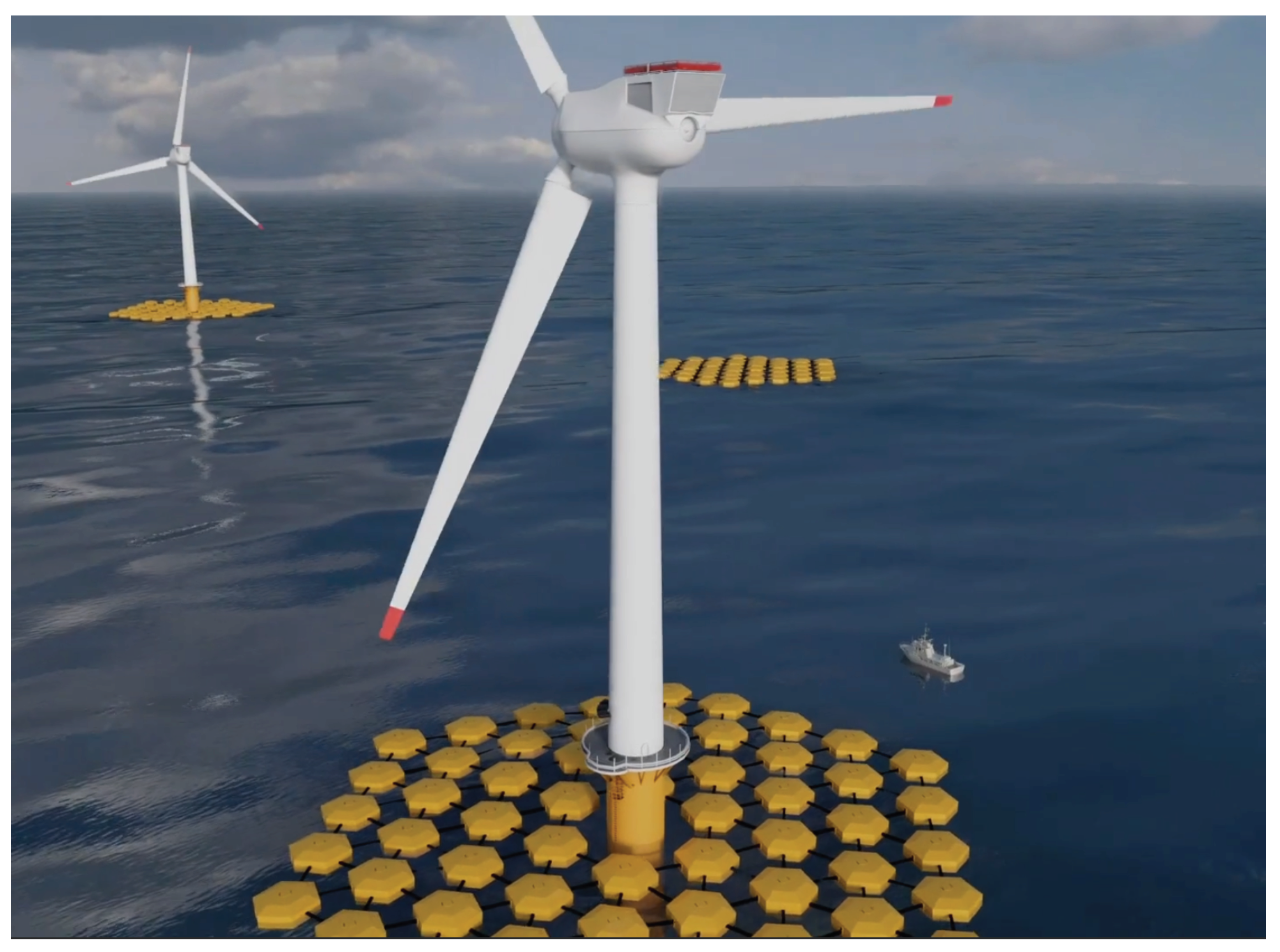
The potential use of arrays of floaters to extract energy from waves has attracted the attention of the wave energy industry as well. For example, the Dutch company Ocean Grazer has recently proposed several versions of its “floater blanket” concept, an array of floater elements each connected to power take-off (PTO) systems [
9]. For details on the technology, see [
10]. An artist’s sketch of Ocean Grazer’s floater blanket concept is illustrated in
Figure 1.
In this paper, we propose a novel mathematical model of wave energy extraction by means of flexible floaters (
Section 2). The technology investigated here would correspond to a column of floaters along the incident wave direction, in the case of the Ocean Grazer WEC. The mathematical model investigates a two-dimensional flexible plate floating on the surface of the ocean, and connected to a series of linear PTO devices. By coupling the method of dry modes with a matched eigenfunction expansion, we show that the energy extraction efficiency of the device is enhanced by the bending elastic modes of the plate (
Section 3). We also show novel results of a demonstrator model of flexible wave energy device made by silicone sheets (
Section 4). The tests were carried out in the Faculty of Science and Engineering, University of Groningen (The Netherlands). To estimate the energy extraction potential of the device, we connected the flexible floater to a 1:35 scale model of the PTO system employed by the Ocean Grazer device. Interestingly, our experimental results show that energy absorption levels are very similar for a continuous floater and a series of single floaters of the same overall length. Finally, the mathematical model is extended to investigate the device performance in random seas. We show that the peak performance decreases in irregular waves, as compared to the monochromatic case. However, the system becomes more efficient at non-resonant frequencies (
Section 5). We anticipate that these results will be of interest to wave energy companies working on the development of flexible WECs (
Section 6).
2. Mathematical Model
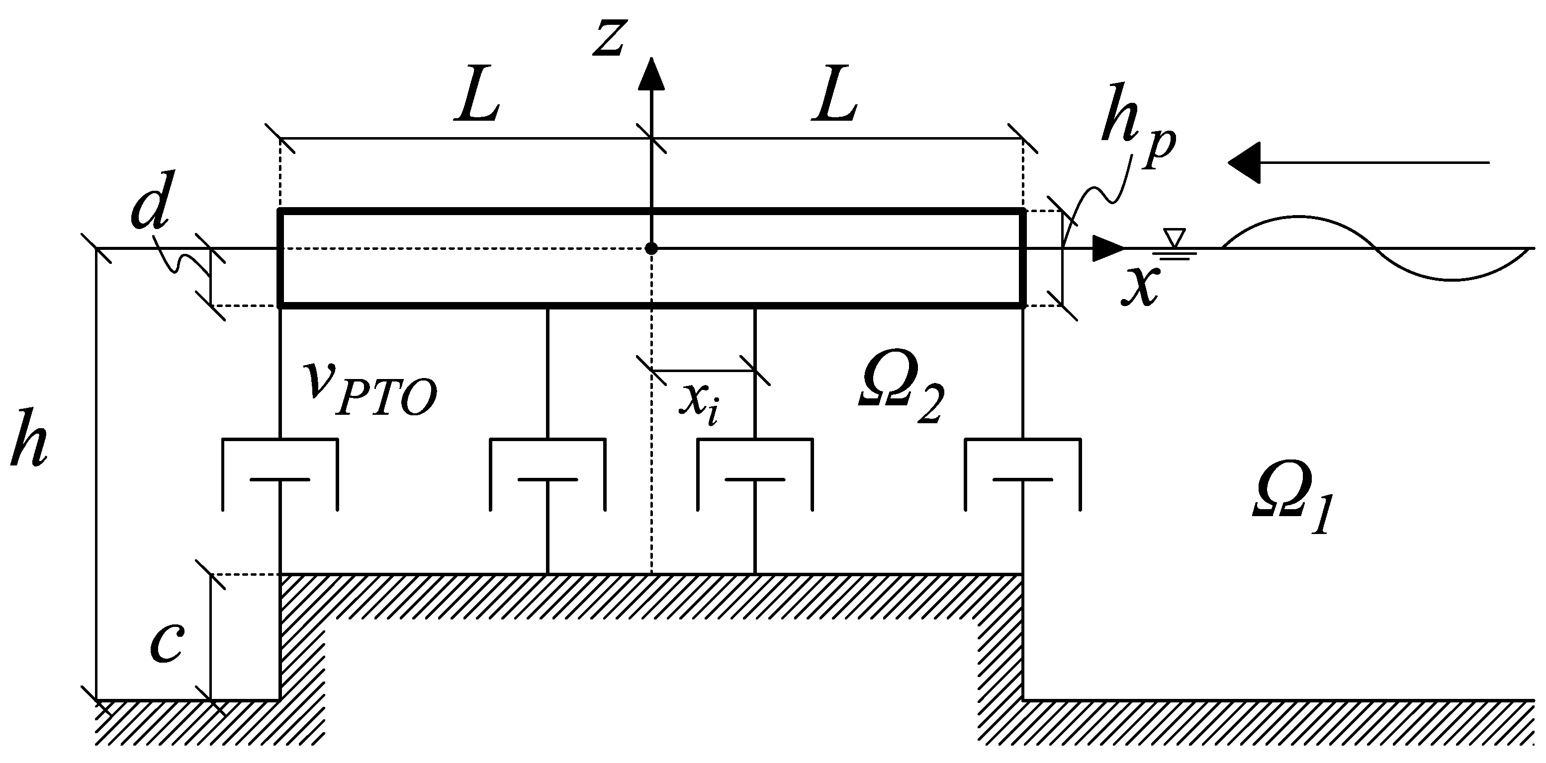
With reference to
Figure 2, consider an infinite two-dimensional channel of constant depth
h and a rectangular ridge of width
and height
c.
Let us define a Cartesian reference system
with the
x axis along the undisturbed free surface and the
z axis positive upward. At
rests a flexible floater WEC of length
and thickness
, allowed to oscillate under the action of incident waves. The WEC is connected to the ridge through a number
M of vertical power take-off (PTO) mechanisms, each with damping coefficient
and located at
,
. We assume
, thus the elastic vibration of the floater can be described by the Euler beam equation [
11]. We assume also monochromatic incident waves of amplitude
A coming from
, inviscid fluid and irrotational flow. Hence, the velocity potential
satisfies Laplace’s equation in the fluid domain
. On the free surface, we have the linearised kinematic and mixed boundary conditions
where
is the free-surface elevation,
g is the acceleration due to gravity and
t is time. The subscripts denote differentiation with respect to the relevant variable. We require tangential fluid velocity at the bottom and on the ridge vertical walls, located at
, i.e.,
where
n denotes the normal derivative to the relevant surface. The kinematic boundary conditions on the wetted surface of the plate are
where
W is the vertical displacement response of the structure and
is the coordinate of the structure’s centre of mass.
Since the system is forced by monochromatic incident waves of frequency
, we assume harmonic motion
with
being the imaginary unit. We now write the governing equations in terms of the spatial variables only
and require that the velocity potential
is outgoing for
.
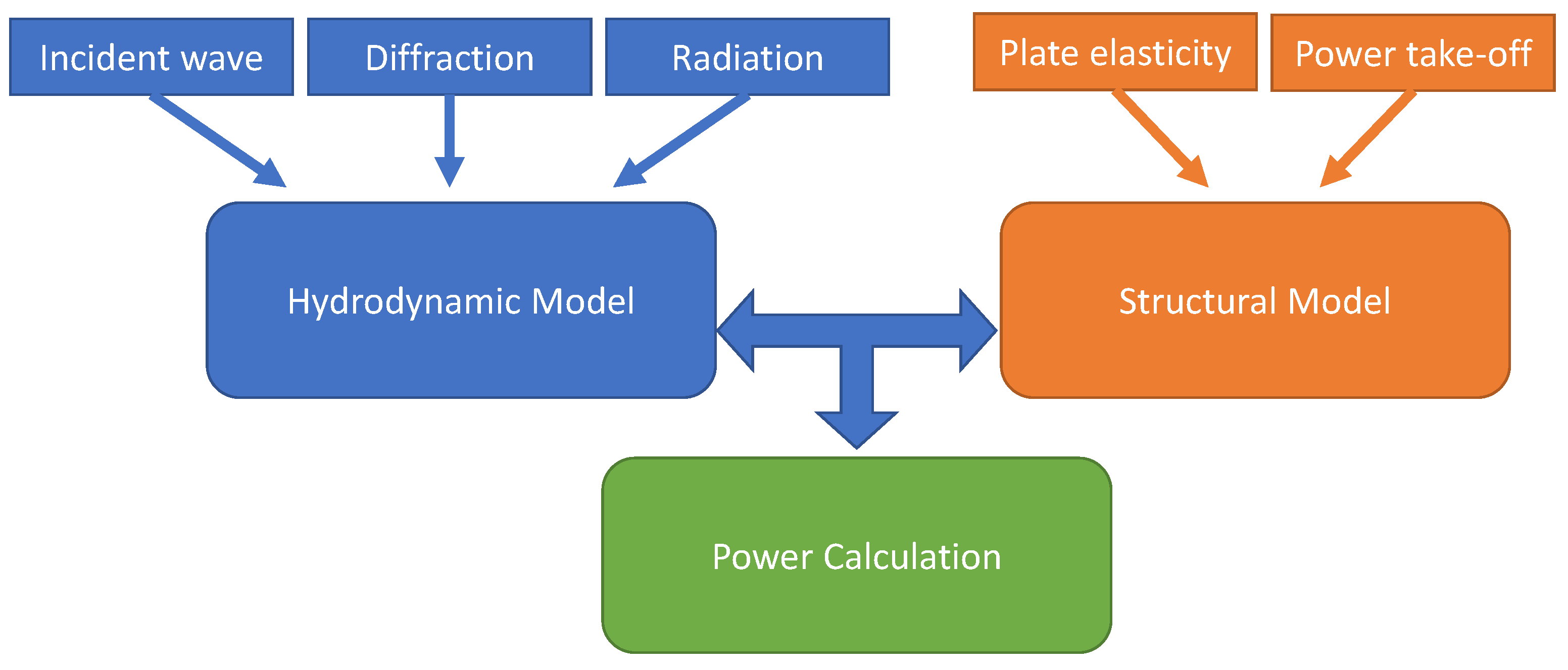
Following Newman [
12,
13], we now decompose the displacement of the floater into a set of dry modes, i.e., in the absence of fluid or added mass. This allows us to significantly reduce the numerical computations and to obtain a deeper physical insight. A schematic diagram explaining our approach is presented in
Figure 3.
Since the plate and the fluid domain are symmetric with respect to the vertical axis
, we decompose the modal expansion into symmetric and antisymmetric parts, hence
where the superscripts
S and
A denote, respectively, the symmetric and antisymmetric components, while
represents the complex amplitude of the symmetric or antisymmetric
lth mode. The plate satisfies the Euler beam equation with free-free end conditions; therefore, the corresponding dry modal shapes are
and
where
and
correspond to the rigid modes heave and pitch [
14], respectively, while the eigenvalues
are the positive real roots of the following eigenvalue conditions
We remark that these modes are orthogonal, i.e., the corresponding shapes satisfy the following properties
The decomposition into symmetric and antisymmetric parts allows us to analyse the half-problem in the region
and simplify significantly the mathematical structure. Let us define the following fluid subdomains
where
represents the domain to the right of the elastic plate, while
represents the fluid region between the elastic plate and the ridge. Following the method of [
15], we decompose also the velocity potential into diffraction and radiation components, i.e.,
where
(
) is the symmetric (antisymmetric) scattering potential,
(
) is the symmetric (antisymmetric) diffraction potential satisfying the boundary conditions (
8)–(
12) with
, and
(
) is the
lth symmetric (antisymmetric) radiation potential for unit amplitude that satisfies the same conditions with the unknown vertical displacement
. The incident wave potential is given by
where the wavenumber
is the real root of the dispersion relation
Now omit the superscripts for the sake of brevity, and let () be the diffraction (radiation) velocity potential in and () the diffraction (radiation) velocity potential in .
The boundary value problem for the subdomain
is
where (
32)–(
33) represent, respectively, continuity of the velocity field and pressure between the fluid domains
and
. The boundary value problem for the subdomain
is governed by
and the coupling matching conditions (
32)–(
33).
In the following sections, we determine the diffraction and radiation potential in and , respectively, by matching the potentials at the common boundaries.
2.1. Diffraction Potential Solution
The general solution in
is given by
where the
are unknown complex constants,
is the set of orthogonal vertical eigenfunctions
denotes the
x dependence
while the terms
’s are the roots of the dispersion relation [
15]
The solution in the domain
below the elastic plate reads
where the
are unknown complex constants and
Usage of the boundary conditions (
32)–(
33) gives
Multiplying each side of (
46) and (
47) by
and
, respectively, and integrating over the relevant intervals,
and
, yields the following inhomogeneous linear systems in the unknown coefficients
and
where
is the Kronecker delta, while
Systems (
48) and (
49) are solved by truncating and numerically solving an
system of equations. The singularity at the bottom edges of the WEC is weaker than that of objects characterised by sharp corners, thus the numerical convergence is fast [
16,
17,
18]. In
Section 2.3, we check the numerical computations through theoretical integral relations, such as the Haskind–Hanaoka formula.
2.2. Radiation Potential Solution
Since the problem is linear, the solution in
can be written as
where the
are unknown complex constants, while the eigenfunctions
and
are given by (
39) and (
40).
The solution in
is given by the homogeneous part and a particular solution that accounts for the plate vibration in
where
are unknown complex constants, while
and
are expressed by (
43) and (
45). The particular solution for the rigid heave mode reads
while the particular solution for the pitching mode is given by [
14]
For the symmetric and antisymmetric
lth bending mode (
15)–(
17), the particular solutions are
As in the previous subsection, continuity of pressure and velocity (
32) and (
33) gives
As in the case of the diffraction potential, by multiplying each side of (
58) and (
59) by
and
, respectively, and integrating over the relevant intervals,
and
, yields the following inhomogeneous linear systems in
and
In the latter,
and
are given by (
50) and (
51), while the constant terms on the right hand side read
As in the previous section, the linear systems (
60) and (
61) are solved numerically by truncating the series at
and
.
2.3. Structural Response and the Haskind–Hanaoka Formula
The vibration of the floating elastic plate is governed by the following Euler dynamic equation
where
E is the elastic modulus of the plate,
I is the area moment of inertia of the plate and
denotes the Dirac delta function. The first term in the equation above represents the flexural rigidity, the second term is the dynamic pressure exerted by the diffracted and radiated wave fields, the third term represents the effect of localised forces due to the PTO system, the fourth term is the hydrostatic contribution, while the last term represents the inertia of the plate.
By expanding
W through the dry mode decomposition (
13) and recalling that for a free-free beam in the absence of applied loads
we obtain
where,
is defined by
The complex coefficients
and
can be found by multiplying the latter equation by
and
, respectively, and then integrating along the total length of the plate
. Truncating the series at
, we obtain a
non-homogeneous system in
and
that can be written in compact form
where
,
,
,
and
are the generalised stiffness matrix, mass matrix, added mas matrix, radiation damping matrix and PTO damping matrix, while the term at the right-hand side represents the exciting force vector. Their respective expressions are given in
Appendix A.
The structure of the latter equation suggests that the floating plate behaves as a linear forced harmonic oscillator. The natural modes of the WEC are then evaluated from the following homogeneous unforced and undamped system
By equating to zero the determinant of the coefficient matrix, we obtain the eigenfrequencies and the respective modal forms.
Now, we apply the Haskind–Hanaoka formula valid for two-dimensional domains to check the numerical computations of the diffraction and radiation velocity potentials. Its expression reads [
15]
where the term on the left hand side represents the exciting force given by (
A21) and (
A22), i.e.,
is the group velocity,
while
is the amplitude of the radiated waves at large distance from the plate, for unit modal amplitude and in the direction opposite the incident waves
in which
is the first complex coefficient of the radiation potential in
(
52). Substitution of (
73) in (
70) gives
The latter relates the diffraction to the radiation potential, and it is used to perform numerical check evaluations.
2.4. Wave Power Extraction and Theoretical Maximum Efficiency
Once the complex coefficients
and
are determined, the average power absorbed over a wave period
by the plate in monochromatic waves can be calculated as
which, after the substitution of (
13), becomes
Then, we define the capture factor as the ratio between the power output
P and the incident wave energy flux per unit width
where
is the total energy and
is the group speed.
We now turn to the evaluation of the theoretical maximum capture factor. Using the radiated wave amplitudes (
73), the most general expression of the capture factor (
77) for two-dimensional flexible floaters becomes
where
denotes the complex conjugate of
, while the superscripts
denoting symmetric and antisymmetric components are omitted for brevity. If there is one degree of freedom, the latter becomes
which is maximised when
. The maximum value of the capture factor occurs when
, i.e., for
and is equal to
. This result can be derived in a different way directly from the equation of motion of a two-dimensional rigid absorber properly constrained [
15,
19].
We remark that the theoretical maximum of the capture factor for a two-dimensional WEC cannot be larger than 1 because of conservation of energy. The plate considered in this work is elastic and characterised by two rigid modes (heave and pitch) and an infinite set of bending modes, thus can be maximised several times within the range of frequencies of interest.
For example, let us consider two modes that dominate the dynamics with respect to the others, one symmetric and the other one antisymmetric. Recalling that wave energy extraction is optimised when the total scattered and radiated waves are maximised in the direction opposite to the incident wave field, we assume
,
, i.e., the radiated wave amplitude of each mode in the direction opposite to the incident waves is the same. The corresponding capture factor becomes
The capture factor is maximised when the first term on the right-hand side is real and negative and when the modal coefficients
satisfy the following condition
Substitution of (
83) into (
82) gives
, a value independent of the WEC size. This result has been obtained from the simplified assumption of WEC motion dominated by two modes, while the flexible floater considered in this work includes rigid and bending elastic modes as well. This aspect potentially implies multiple optimisation and consequent larger efficiency with respect to standard rigid devices.
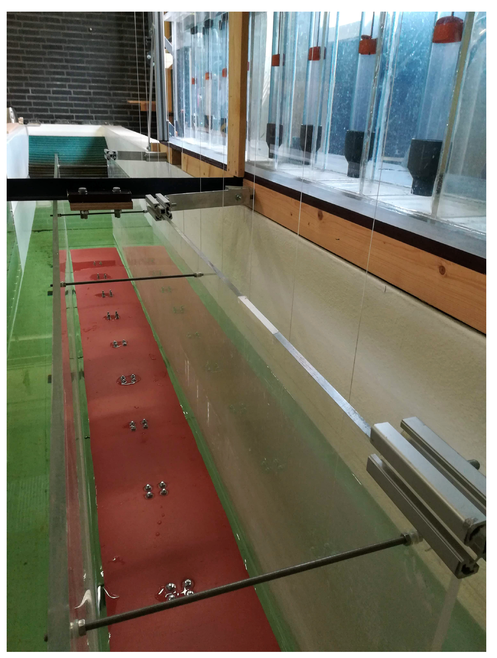
4. Comparison with Preliminary Demonstrator Data
The flexible floater demonstrator is made by two layers of Polymax SILO-CELL silicone sponge sheet, each of dimensions 2 m (length) ×
m (width) ×
m (thickness), see
Figure 7.
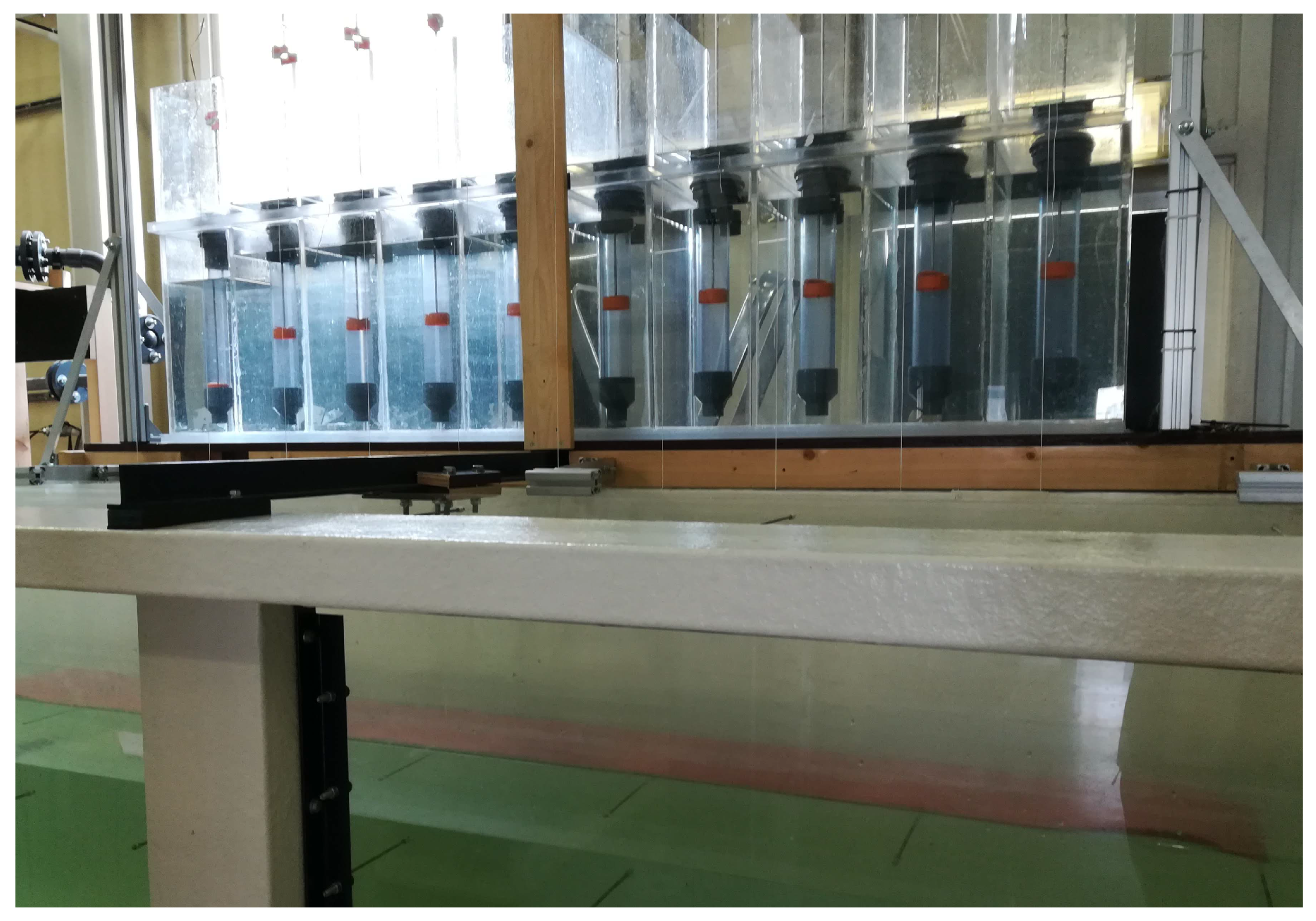
The floater is attached to a laboratory model (scale 1:35) of the multi-pump, multi-piston power take off system (MP
PTO) designed by the University of Groningen and Ocean Grazer, shown in
Figure 8.
The MP
PTO system is installed inside a wave tank, which is
m high,
m wide and 10 m long. Two transparent lateral walls are also installed inside the wave tank, along the direction of the incident waves, restricting the width to
m. This effectively creates a channel inside the tank, and the flexible floater is then installed inside this channel. The channel width matches the floater width (
m), hence the dynamics inside the channel are two-dimensional. The water level in the tank is
m. The waves are generated by a flap paddle driven by a rotating-arm engine, located at one side of the tank. The engine frequency and the length of the rotating arm can be set to a maximum of 60 Hz and
m, respectively. At the other side of the tank, a plane beach induces wave breaking, thus dissipating wave energy and reducing reflection. To calibrate the wave maker, digital particle image velocimetry (DPIV) measurements were taken using a high-definition camera. The camera recorded the motion of tracer particles (polyamide particles) seeded in the tank, which was illuminated by means of a laser sheet. For details on the measurement procedure and associated errors, we refer the interested reader to Refs. [
25,
26] and references cited therein. The system of pistons and cables was calibrated using load cells, as described in Ref. [
27].
4.1. Description of the Demonstrator Device
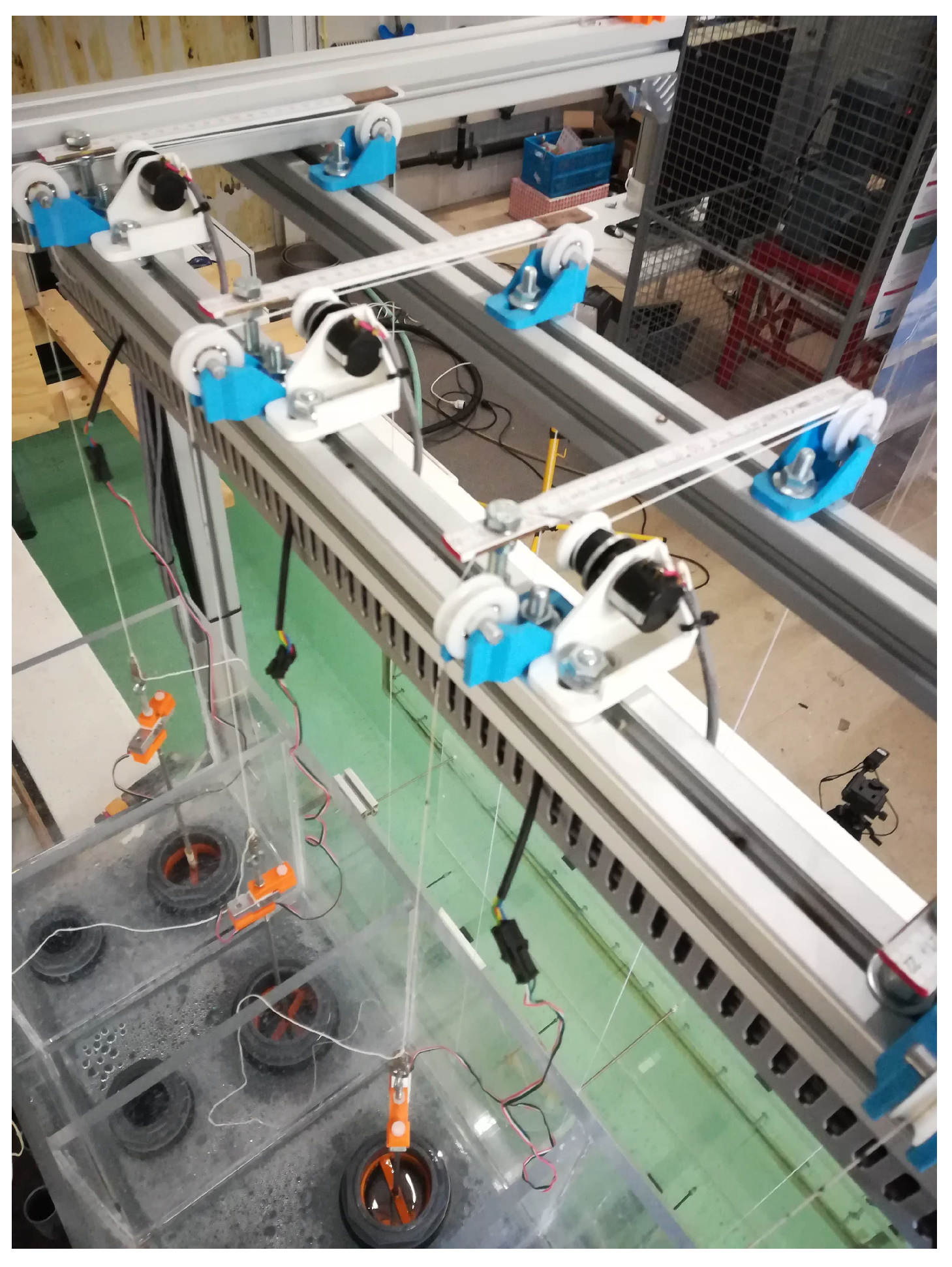
The flexible floater is connected to the MP
PTO system in the tank via high-performance polyethylene cables, which are in turn connected to pistons. Each piston is located inside a
m wide cylinder. As the floater deforms under the action of the incident waves, it transmits its motion to the pistons via the cables. In turn, the pistons pump water inside the cylinders, as shown in
Figure 9.
The power extracted by each PTO element can be approximated by calculating the work done by the piston against the force of gravity to lift the water column of weight
, where
A is the cross-sectional area of the cylinder and
H is the maximum hydraulic head over a cycle. Thus, the extracted power is given by
where
is the duration of the upstroke motion of the piston.
Four sets of demonstrations are conducted. In two sets (S1 and S2), the floater is a continuous flexible silicone sheet of 2 m length, whereas in two sets (S3 and S4), the floater is cut into 10 pieces, each being
m long and connected to a single piston. For each setup, the maximum hydraulic head in each cylinder is measured eight times, and the average of such measurements is then taken. The engine and wave parameters for the four sets of tests are reported in
Table 1. We use Froude’s law to scale between test and model results. The Froude number is
where
U is the fluid speed and
D any linear dimension of the system. Using Equation (
84) and a 1:35 scale ratio, the wave periods
s and
s scale up to 8 and
s, respectively, whereas the wave heights
m and
m scale up to
m and
m, respectively. These values are consistent with an oceanic wave climate, such as the North Atlantic Ocean [
28].
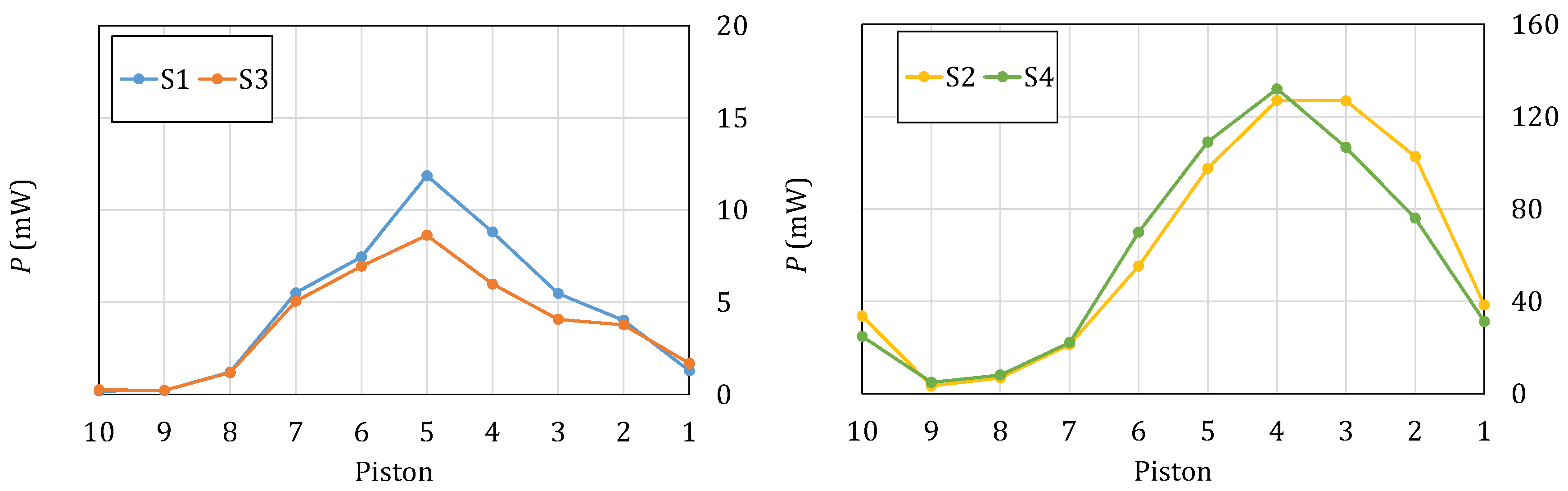
4.2. Demonstrator Results
Figure 10 shows the average power at each of the 10 pistons in the MP
PTO laboratory model, for the four sets of tests detailed in
Table 1. Piston 1 is the closest to the generator, whereas piston 10 is the closest to the absorbing beach, on the other side of the tank. Note that, in all configurations, the power absorbed by the device first increases moving towards the centre of the floater, and then decreases moving further on. Therefore, in all cases, the maximum power output is achieved towards the middle of the floater. Note also that the power has a second maximum at the tail of the floater (piston 10), which results from end reflections by the inclined beach. This is especially visible in the more energetic sea state (configurations S2 and S4), whereas it is almost negligible in the milder sea state (configurations S1 and S3).
As expected, the configurations relevant to the more energetic seas, S2 and S4, are also those with the largest power.
Figure 10 also shows that the maximum power attained by the continuous floater (configurations S1 and S2) is similar to that achieved by the discontinuous floater (configurations S3 and S4). Interestingly, in the less energetic state, the continuous floater (configuration S1) performs slightly better than the discontinuous one (configuration S3) at almost all pistons. In the more energetic sea state, the continuous floater (configuration S2) performs better than the discontinuous one (configuration S4) towards the front (pistons 1,2 and 3), and worse towards the middle (pistons 4–9). Since there is no substantial advantage in choosing the continuous configuration over the discontinuous one (at least in the sea states analysed here), our results suggest that in practice one can opt for either configuration based on other criteria, such as installation and maintenance costs. In this sense, the discontinuous configuration appears more advantageous to reduce maintenance costs, for example due to the possibility of replacing only one element, instead of the whole floater, in case of localised damage. The positive practical implication of our preliminary findings prompts the need to scale-up the demonstrator device to a full-fledged experimental model. This is the object of our ongoing research effort.
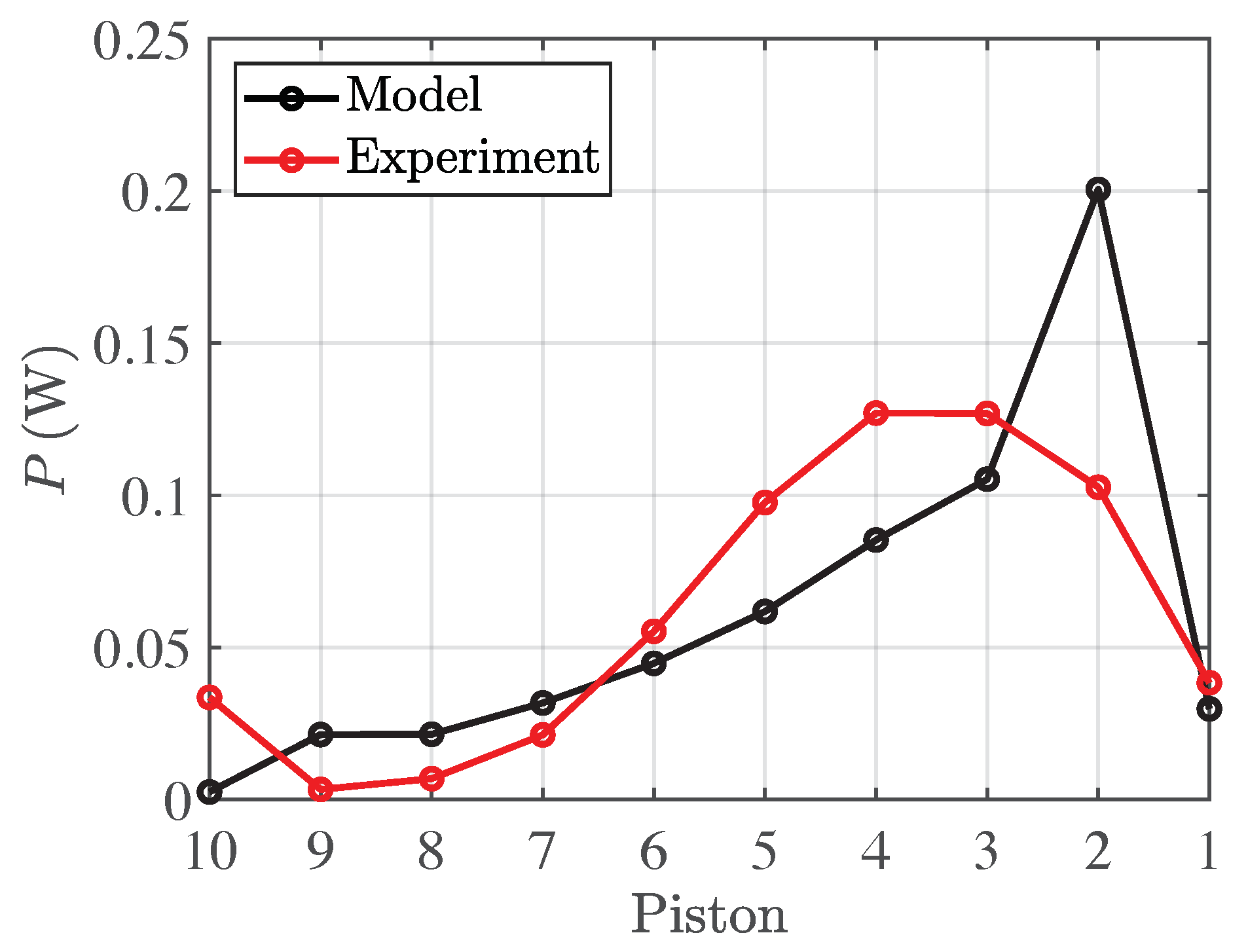
4.3. Comparison with Mathematical Model
In this section, we show a preliminary comparison between the results of the experimental and mathematical models. We remark that the PTO system is modelled as a linear damper in the mathematical model, whereas it is nonlinear in the experimental model. For the sake of comparison, we selected a PTO coefficient for the model which generates the same total power output as that in the demonstrator device. This allows some quantitative comparisons and discussions.
Figure 11 shows the behaviour of the power output for each piston, in both the mathematical model and the tests, for the same configuration as
Figure 10. The overall behaviour is captured well and, in general, the comparison is satisfactory. Both models show that the maximum power output is achieved by those pistons located towards the front of the device. Some differences (especially in the maximum power output) still remain, and these are likely due to the use of a linear PTO in the mathematical model.
We remark that, to date, very few studies have investigated the non-linear dynamics of wave-plate systems analytically, see for example Refs. [
29,
30]. However, these dealt with the interaction of waves with ice sheets. On the contrary, to the best of our knowledge, no application of nonlinear theories to wave power extraction from flexible plates has been made so far. This highlights the need for developing higher-order mathematical models to achieve a more accurate description of the power extraction dynamics.
5. Power Extraction in Irregular Waves
In this section, we investigate the effect of irregular sea waves on the floating plate dynamics and power extraction efficiency. Let us assume the following JONSWAP spectrum function [
31]
in which
is the significant wave height,
denotes the peak frequency and
Since the problem is linear, the oscillation of the flexible plate can be written as
where
is the
nth component of the discretised spectrum,
is the frequency interval,
is a random phase related to
, whereas RAO is the response amplitude operator for the plate, i.e.,
Then, the instantaneous generated power by the entire system is
From the previous expression, we obtain the averaged generated power [
17,
20,
22]
whose expression in the limit
becomes
Defining
as the total incident wave power per unit crest width
the capture factor in irregular seas
can then be written as
The latter expression gives the capture factor for any sea state characterised by significant wave , peak frequency and PTO coefficient .
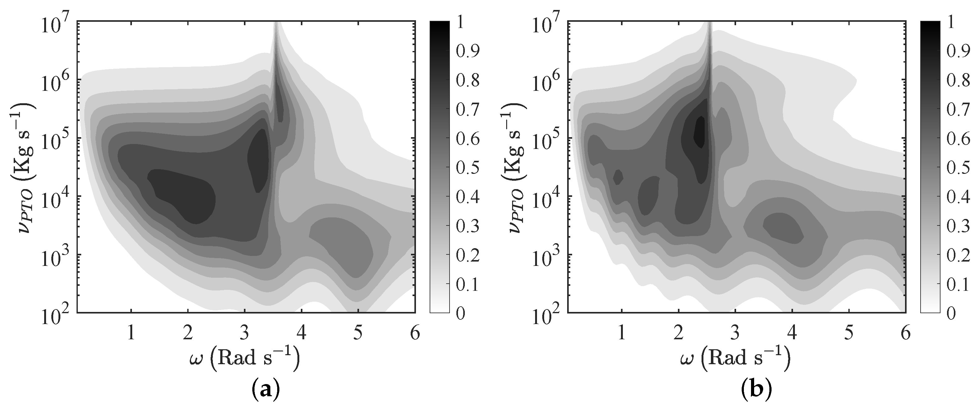
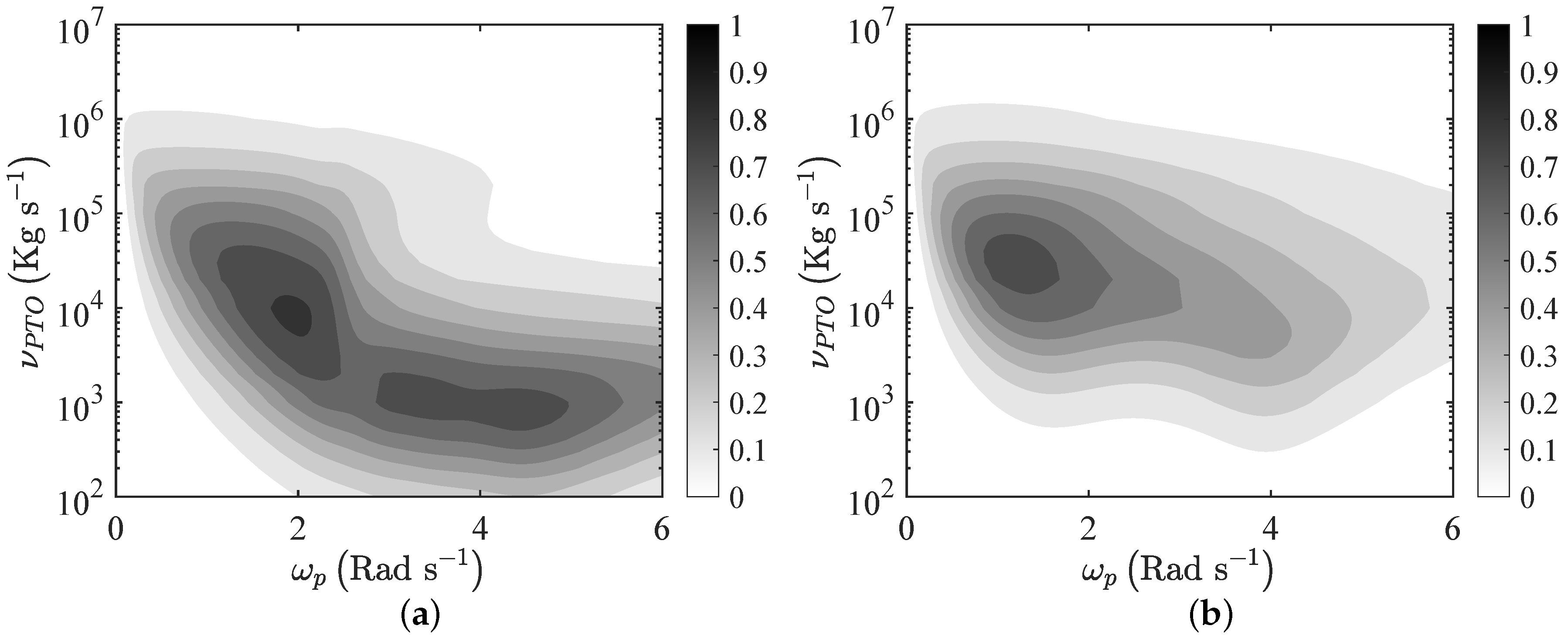
Let us investigate the capture factor in irregular waves of the same plates analysed in
Section 3.3.
Figure 12 shows the behaviour of
versus peak frequency
and PTO-coefficient
for the softened flexible plate and the rigid plate. The softened plate has stiffness factor
kg m
s
, while the rigid plate has
.
As in the case of monochromatic incident waves, the flexible plate results in being more efficient than the rigid plate and can be optimised for several values of and . Indeed, the rigid plate shows a single peak, while the flexible plate shows three maxima and a much larger bandwidth.
In addition, by comparing
Figure 6 and
Figure 12, we note that the maxima are reduced with respect to the case of monochromatic waves, whereas the system can be more efficient outside the resonant frequencies. This is mainly due to the coupling between the broadband incident waves and the eigenfrequencies of the system. Similar results were already obtained in the context of oscillating wave surge converters and oscillating water columns [
17,
20,
22].

 ,
, 


