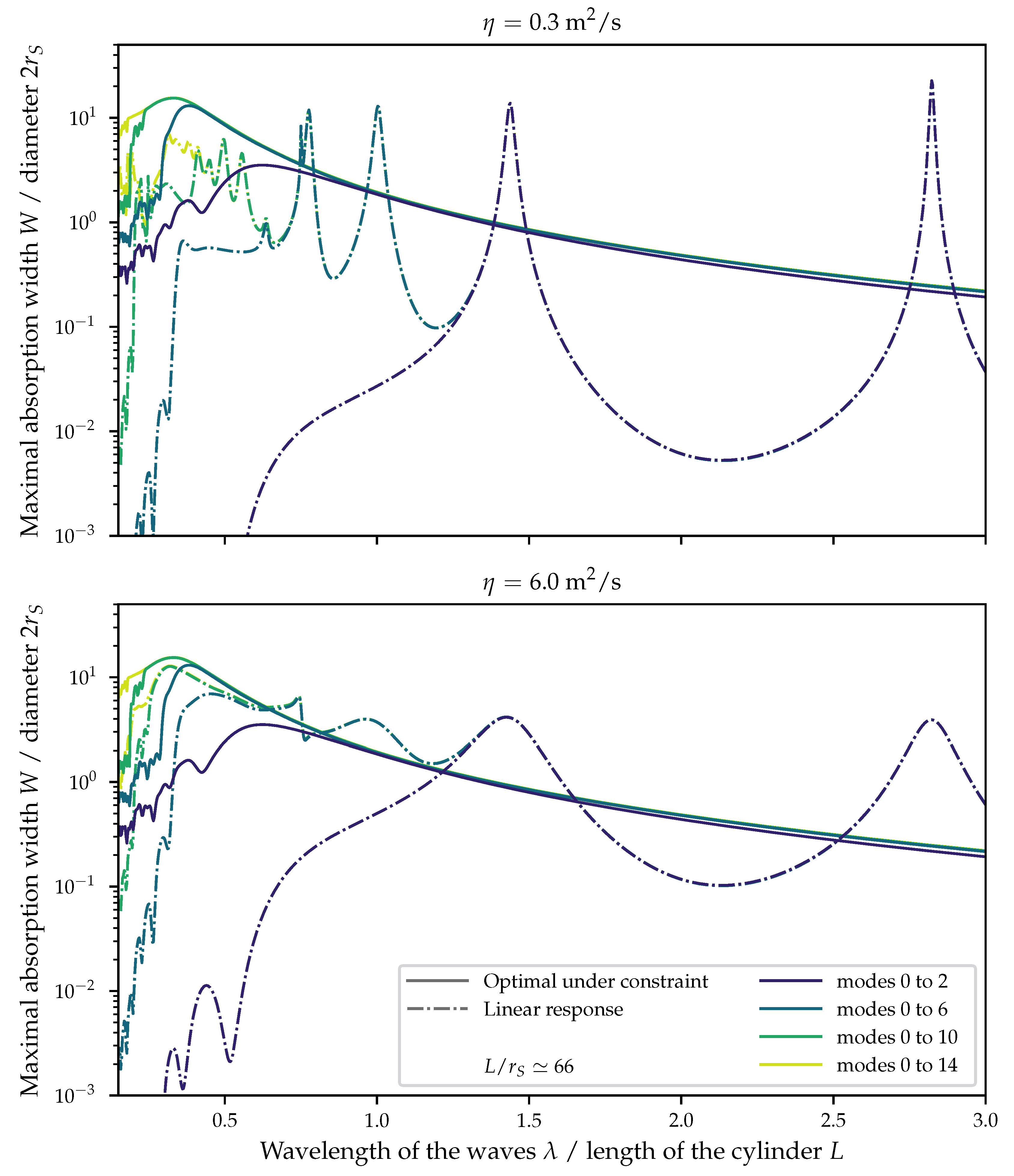
2.1. Far-Field Maximal Absorption Width without Constraint
Let us consider a linear potential flow in the frequency domain. Here, we follow the conventions of [
7] and we refer to that book for more details on the derivation of the following formulas. Note that Newman in [
8] uses a different convention for the definition of the Kochin functions:
, where
k is the wavenumber. The convention for time dependence is also different:
whereas it is
in this paper, where
ℜ is the real part. For the sake of simplicity, all of the computations in this paper are performed assuming an infinite water depth, although similar formulas exist in the finite depth case.
In the far field, the radiated wave can be described by the complex-valued Kochin function
, where
is a direction of interest. It can be related to the complex-valued velocity potential
in cylindrical coordinates
as
where
is a function of the vertical coordinate
z only and
is the wavelength of the waves.
Because we consider a linear problem, the potential of the radiated waves and the associated Kochin function can be decomposed as a sum of contributions from each dof taken independently. In the frequency domain, a body motion is defined by complex values that represent the amplitude of the dof j. We can then write , where is the Kochin function for a unit excitation of the dof j.
We use the absorption width W to measure the efficiency of the WEC. It is the ratio between the mean absorbed power (in watts) and mean power flux of the incoming waves (in watts per meter). Thus, it has the dimension of a length.
By writing an energy balance around a WEC (Equation (4.21) of [
7]), we can derive an expression for the absorption width
W. Assuming incoming waves with a complex-valued amplitude
and a WEC oscillating with complex-valued dof amplitudes
, we have:
where
ℑ is the imaginary part, the star denotes the complex conjugate,
k is the wavenumber, and
is the direction of the incoming waves (in radian).
The first term of (
2) depends on the Kochin function downstream of the WEC as well as the phase of
, which is the difference of phase between the motion of the dof
j and the incoming waves. The second term of (
2) is the total amount of energy lost by radiation by the WEC in all directions and is independent of this difference of phase.
Diffraction does not explicitly appear in (
2). Physically, it can be understood by the fact that no energy can be absorbed by a fixed non-radiating body. Mathematically, we refer to Equation (4.20) of [
7].
The above expression can be reformulated in the following way. Let us consider a floating body in free motion in a wave field. Part of the incoming energy is dissipated or captured by the device, while the rest escapes in the diffracted and radiated fields. Let us now force the exact same motion to the same WEC in a still ocean without incoming waves. The pattern of the waves radiated by the forced body is sufficient to compute the power that was dissipated or absorbed in the free motion experiment. Analyzing all of the wave patterns that can be radiated by a body with a given shape gives us a clue on the maximal power that could be absorbed by a body with such a geometry.
The above expression relates a given motion of the WEC to the power absorbable by this motion for a given wave field
. The maximal absorbable power can be found as the maximum over all possible motions of the body. The maximal absorption width reads
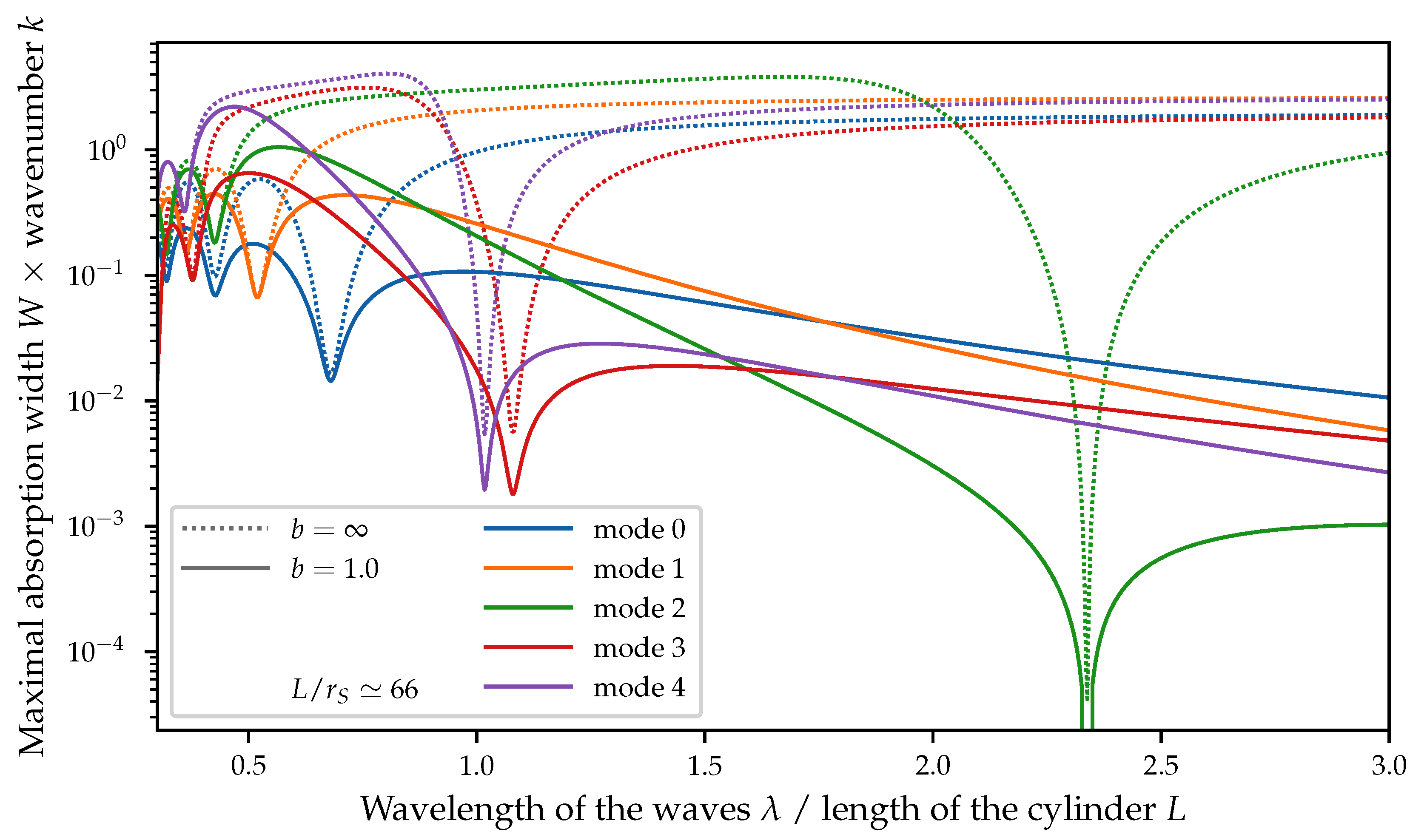
The absorption width only depends on , so the solution for all can be deduced from the resolution of the problem for a single value of .
Besides, this optimization problem can be slightly simplified thanks to the following remark: for a given motion of the WEC, the first term of (
2) varies with the difference of phase between
and
as a sine function between
and
. When we are looking for the best absorption width, the difference of phase can be assumed to be optimal and the first term maximal. We will denote this situation as the WEC being
in phase with the incoming waves.
Using this fact, we can rewrite (
3), as
where
is defined as
This analytical optimization of the difference of phase between the WEC and the incoming waves reduces the dimension of the space of candidate motions from to .
For a single dof (
, the absorption width
W is a quadratic function of
, where
is the complex-valued amplitude of the dof. This function has a maximum
, which reads (also see [
8])
Using the assumption of a slender body, Newman [
8] and Farley [
9] have derived analytical expressions for the maximal absorption width for a deformation along a single dof.
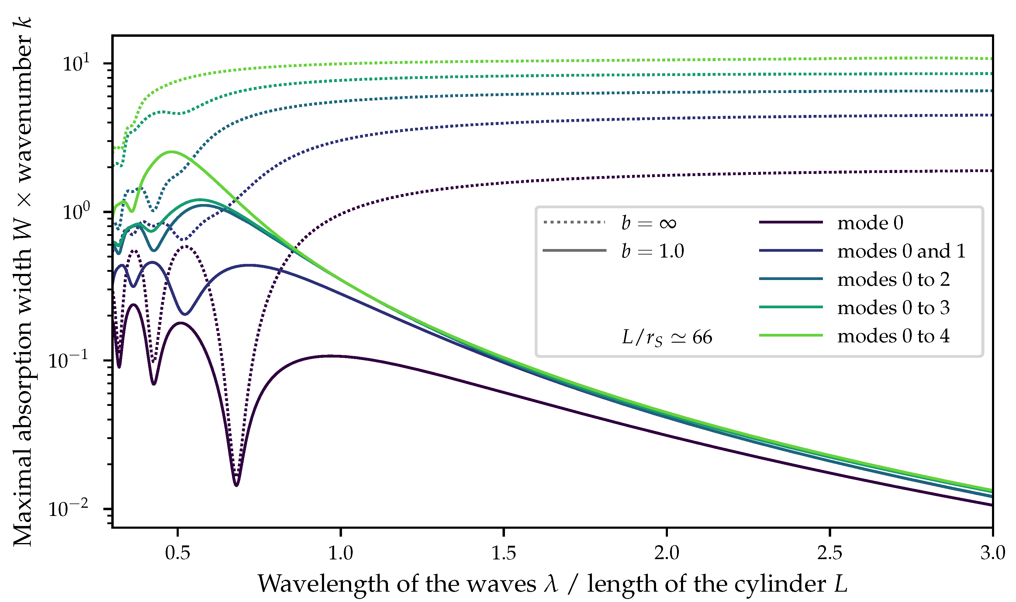
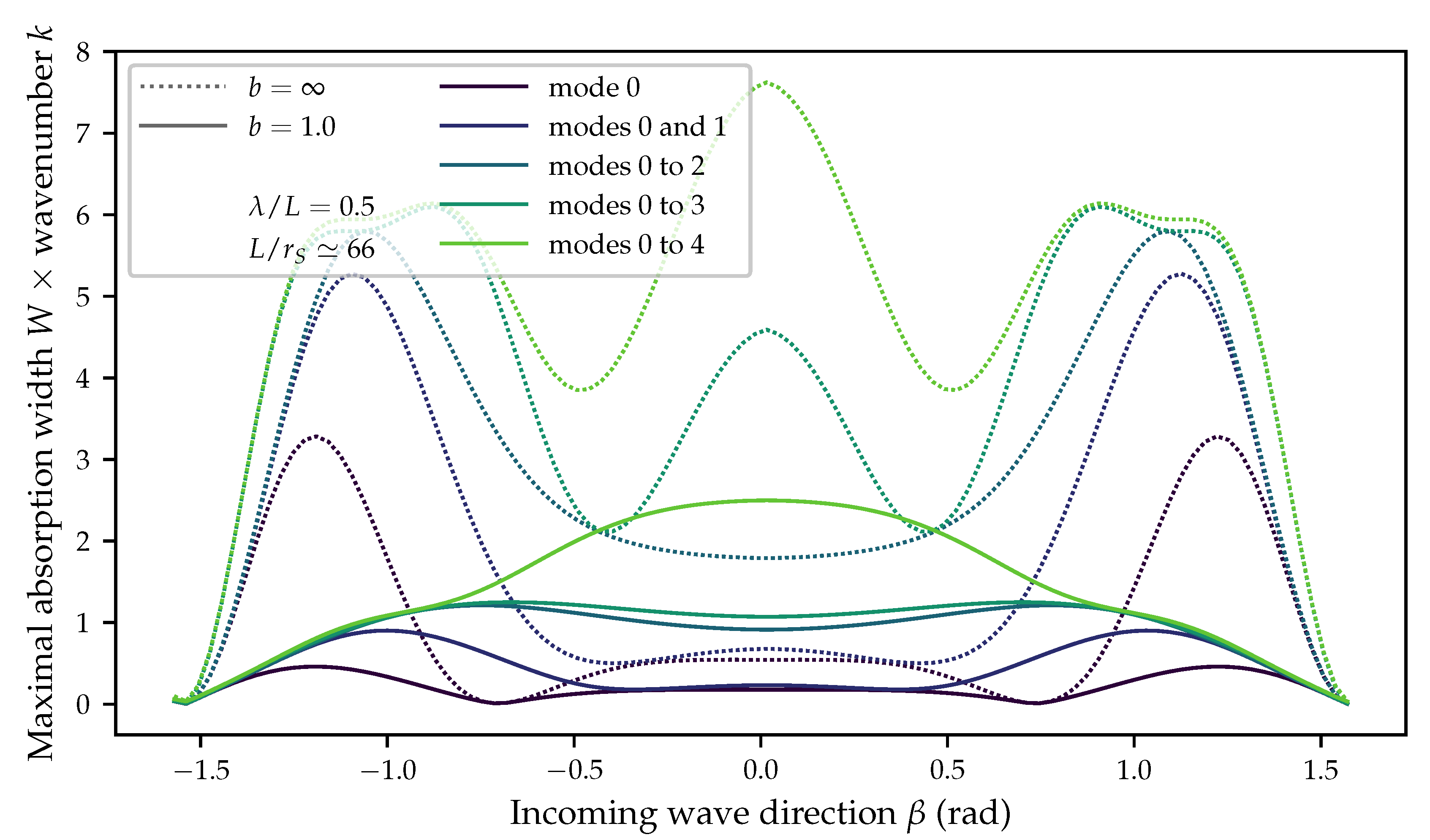
A generalization of (
6) for several dofs can be found in Equation (4.24) of [
7]. It takes the form of a complex-valued linear system of
equations, since the function to maximize has the form of a quadratic function of
.
Another relation can be useful for studying the maximal absorption width of a WEC [
13]:
where
is the number of hydrodynamically independent dofs (that will not be distinguished from the total number of dofs in this paper). For a single dof, (
7) can be easily derived from (
6). On average over all incoming wave directions, all of the bodies and dofs have the same maximal absorption width. In [
11], this fact has been illustrated on the example of a simple rigid body moving in heave or in surge. The
of the heaving body is independent of the direction of the incoming waves, whereas the
of the surging body varies as
. It is maximal when the direction of motion and the incoming waves are aligned and zero when they are orthogonal. However, one can check that, on average, over all wave directions, both maximal absorption widths are the same and are independent of the shape of the body.
2.2. Far-Field Maximal Absorption Width under Constraint
If the absorbable power of a WEC was indeed independent of the body shape and of its dofs, as suggested by (
7), all research on wave energy would be simpler. Unfortunately, the reasoning above has several shortcomings. The main one is the following: the amplitude
at which the absorbed power would be maximal is often not reachable by the devices. The amplitude is constrained by, for instance, mooring for translation motion or elastic properties of the material for a deformable WEC. The range on which the electric system can extract energy can also constrain the “useful” amplitude of the dof.
For a single dof, the constraint can easily be taken into account in the analytical expression (
6) (see also [
8]):
where
is the maximal admissible amplitude.
For several dofs, an optimization under constraint problem has to be solved:
where
is the set of admissible motions of the WEC. In this work, the constraint takes the form of a
-norm on the vector of complex-valued amplitudes
, which is
for a given
.
In general, the -norm of does not have a physical interpretation and this type of constraint has only been chosen for its simplicity of implementation in an optimization software. It might be possible to derive an analytical expression for the maximal absorption width under constraint, as in the one-dimensional (1D) case, at least for such a simple constraint. This has not be done in this work, where we used an optimization algorithm to find the optimum.
Without the constraint, the problem is linear, in the sense that it only depends on
. With a constraint, such as (
10), this is not the case anymore: the amplitude of the incoming waves and the amplitude of the body motion are independent. In the rest of the paper, we will keep working with the normalized amplitude
and apply the constraint in the following form:
The constraint on the right-hand side of Equation (
11) means that the change of the amplitude of the incoming wave is equivalent to a change in the constraint
b. Indeed, when the amplitude of the waves is small, the system will be able to capture the incoming energy without breaking the constraint and the problem can be seen as unconstrained. On the other hand, cases with high wave amplitude will be more affected by the constraint of the body motion.
2.3. Modal Analysis of the SBM Offshore’s S3 Device
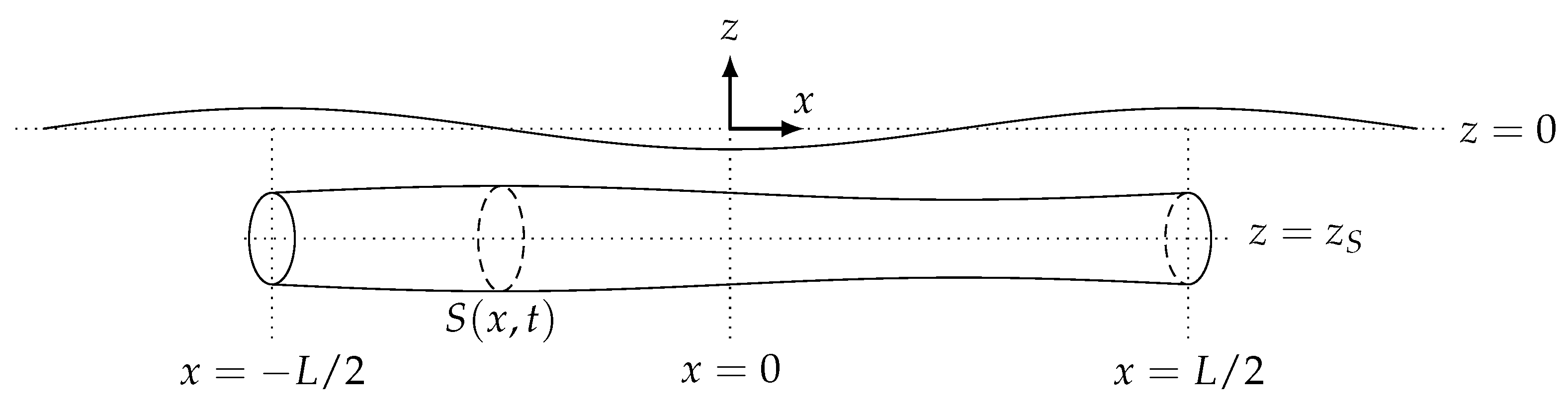
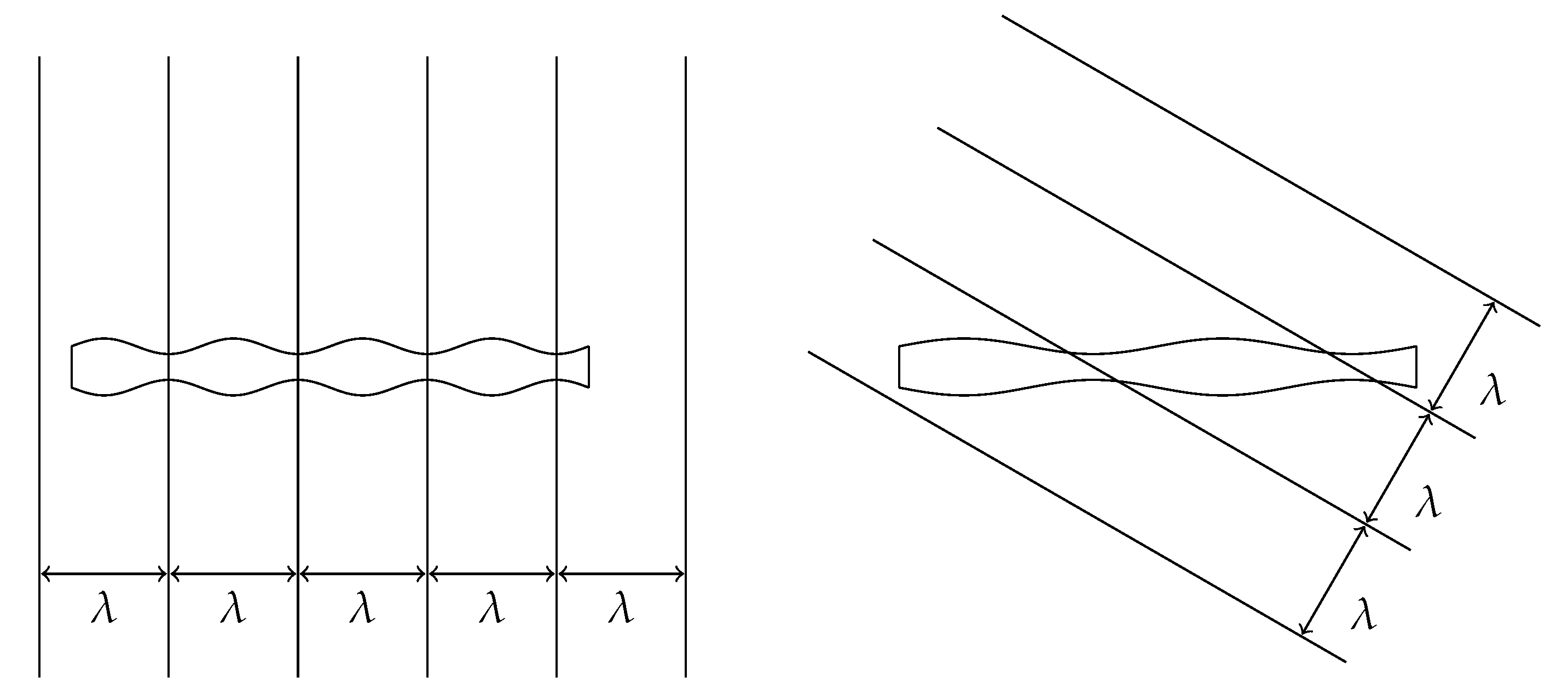
The S3 device consists of a water-filled horizontal elastic tube floating just beneath the sea surface. When ocean waves travel above it, they apply a time-varying pressure on the tube wall that induces local changes in diameter. This creates bulge waves in the tube. Subsequently, the elastic deformation is converted into electricity thanks to its electroactive attribute.
We model the device as a horizontal cylinder, parallel to the free surface, with
the depth of its axis. Let
L be the length of the cylinder (constant) and
its cross section at rest (that is when the device is immersed but static). The cylinder is modeled as a one-dimensional (1D) system (since
) and its deformation is assumed to be axisymmetric. We denote, by
, the cross section at position
and at time
t (see
Figure 1 for a schematic of the system).
Following Babarit et al. [
5], we define
, such that
, where
U is the velocity of the fluid inside the cylinder. From mass conservation, one has
Because we are studying the linear regime of small deformations, the radial motion of a point on the surface of the cylinder can be computed as
where
is the radius at rest.
Neglecting the damping and the interaction with the outer fluid, the following wave equation can be derived:
where
D is the distensibility of the membrane,
the tension in the wall of the tube at rest, and
the density of the fluid. We look for a solution of the form
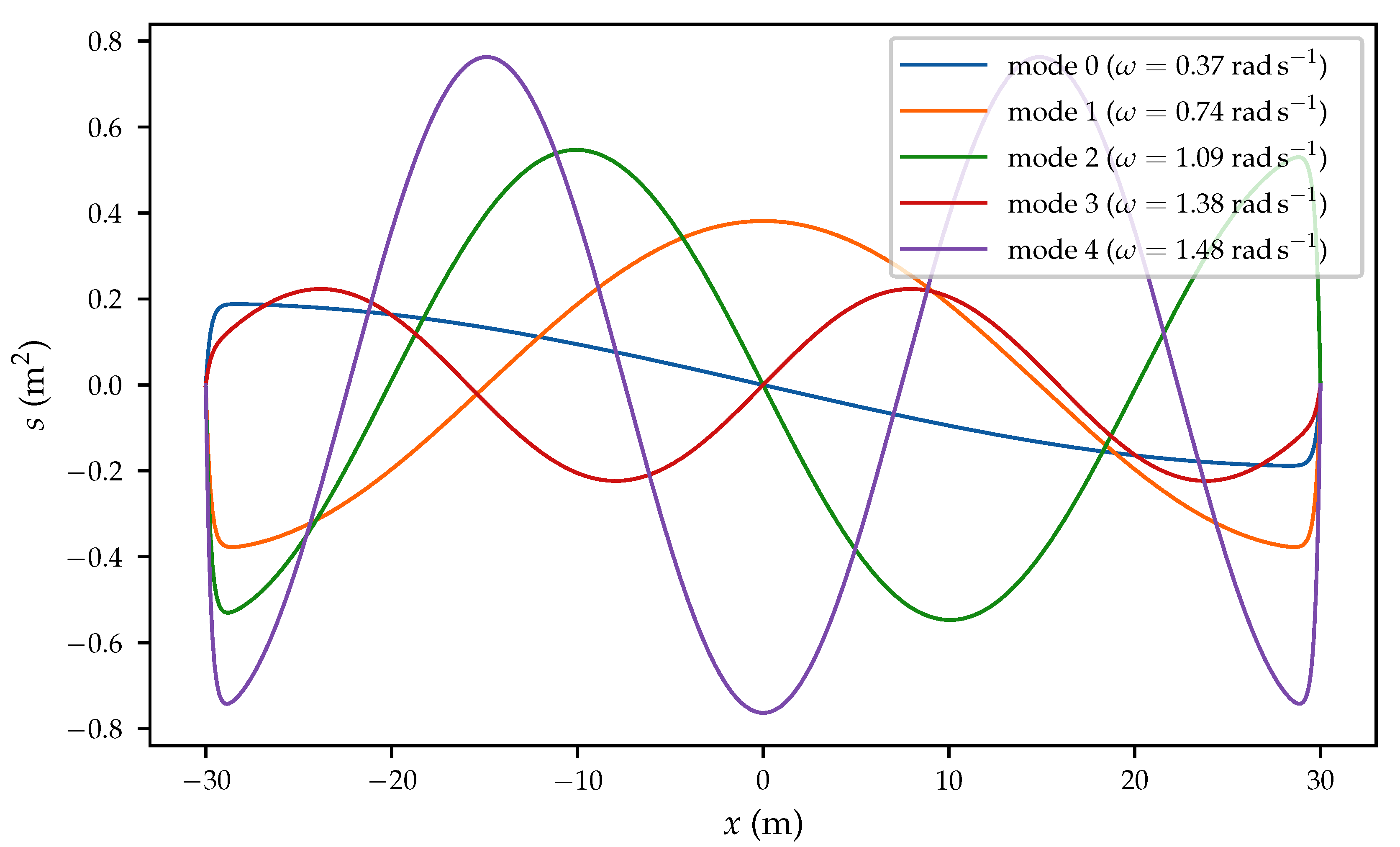
. The resolution is thoroughly developed in Appendix B of [
5]. Modes of deformations
are expressed for each frequency
and wavenumber
satisfying the dispersion relation derived from (
14). The modes are normalized while using the scalar product
Figure 2 shows the first five modes of the WEC that we consider. The parameters used for the model can be found in
Table 1.
By introducing into the full equation of motion of the WEC
where
is the normalized
i-th mode, one obtains the following discrete equation of motion on the coefficients
, where
is the complex-valued amplitude of the dof
i in the frequency domain:
Here,
is the added mass matrix,
is the radiation damping matrix,
is the dissipation coefficient,
is the wall damping matrix
is a damping parameter that is related to viscosity,
is the inner flow damping matrix
is the diagonal matrix of the pulsations of the modes of the cylinder, and
is the excitation force.
The mean power dissipated by the material can be computed as
Alternatively, for a given deformation
, the dissipated power can be evaluated with the help of the far-field Equation (
2). One can check that both expressions of the power give the same results [
12]. A similar comparison is done in [
1,
14].
In the previous section, we discussed the definition of a constraint on the amplitude of motion or deformation of a body. It will take the form (
11) for the coefficients
that are defined in this section. From (
12) and (
16), we have
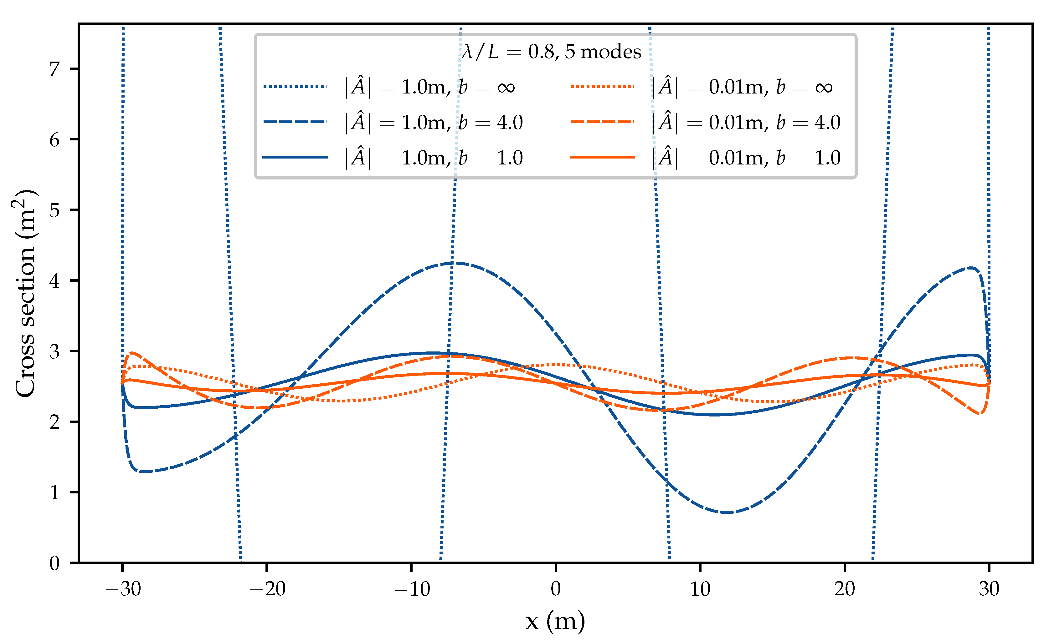
where
is the deformation profile of mode
i, as plotted for instance on
Figure 2. Thus, a constraint on the norm of
can be interpreted as a constraint on the minimal and maximal variations of the cross section
s. However, the exact relationship between
and the norm of
is unknown. (In particular, the normalization using the scalar product (
15) of the modes leads to non-trivial values of
for all
i.) For a given bound
b in (
11), the actual maximal geometrical deformation of the WEC is only checked a posteriori. This is a limitation of the current implementation.


