Energy-Efficient Speed Profile Optimization and Sliding Mode Speed Tracking for Metros

Abstract

Nowadays, most metro vehicles are equipped with an automatic train operation (ATO) system, and the speed control method, combining cruise speed planning and proportional-integral-derivative (PID) control, is widely used. The automation is achieved, and the energy-efficient can be improved. This paper presents an improved artificial bee colony algorithm for speed profile optimization with coast mode and an adaptive terminal sliding mode method for speed tracking. Specifically, a multi-objective optimization model is established, which considers energy consumption, comfortableness, and punctuality. Then, a novel artificial bee colony algorithm named regional reinforcement artificial bee colony (RR-ABC) is designed, to search the optimal speed profile with coast mode, in which some improvements are made to speed up convergence and to avoid local optimal solutions. For speed-tracking control, the adaptive terminal sliding mode controller (ATSMC) is used to improve the speed error, robustness, and energy saving. In addition, a disturbance observer (DOB) is designed to improve the anti-interference ability of the system and further improve the robustness and anti-disturbance, which are also conducive to speed error and energy saving. Finally, the line and train data of the Qingdao Metro Line 6 are used for simulation, which proves the effectiveness of the study. Specific to the energy saving rate, and compared with normal algorithms, RR-ABC with coast mode is approximately 9.55%, and ATSMC+DOB is 7.58%.

1. Introduction

In the modern metro system, the quality of operation, including energy saving, punctuality, and comfortableness, is the core factor for operation [1]. With the popularization of the Automatic Train Operation (ATO) system, the automation of train operation has been achieved. However, the performance of the algorithm in ATO system is not good enough, and it can be further improved [2]. Inaccuracy and high energy consumption seriously affect the quality of train operation.

The frequent switching of operation mode is needed for the metro system because the start–stop is frequent. The ATO system needs to refer to the planned speed profile as a reference to issue control commands, such as acceleration, braking, and coasting [3]. In practice, the PID controller is widely used to realize speed control, and the fluctuation of control force occurs when the coasting mode is needed [4]. This problem eventually leads to larger speed errors and poor energy saving effects. To improve the tracking quality, a large number of papers are published to try to find a perfect substitute of the PID controller. Predictive controller is presented to track the speed profile. In Reference [5], an integral sliding mode control (ISMC) is used to design distributed adaptive control strategies. In Reference [6], a tracking controller is formulated to resolve errors caused by unmolded effects. In References [7,8], a robust adaptive controller is proposed to adapt unknown system parameters and nonlinear traction/braking notches. Wang et al. proposed an approach to design a distributed and fault-tolerant controller which is applied to develop braking control schemes for high-speed trains subject to traction and braking failures [9]. In Reference [10], to deal with input saturation and unknown disturbance in high-speed trains, a neural adaptive fault-tolerant controller is designed. In all the abovementioned studies, either the convergence cannot be proved by Lyapunov theory or the convergence speed is not good enough. In addition, large speed errors in those controllers also result in large energy consumption. Therefore, they are not suitable for metro trains that require fast convergence and high-precision tracking.

Recently, sliding mode control is becoming a research hotspot. Because it is easy to design and did not require accurate parameter identification, it has been used in actual physical systems, such as power systems and industrial robot manipulators [11,12,13]. In addition, the controller with a nonlinear sliding surface has been proven to converge in a limited time [14]. Especially for the adaptive terminal sliding mode controller (ATSMC), in addition to the advantages of fast convergence, it can also be adaptive to the internal parameter disturbance and external interference of the system [15]. Inspired by the above articles, we introduce the additional resistance caused by slope and the basic running resistance of the train into the sliding mode controller, in the form of disturbance, and an adaptive terminal sliding mode controller for train-speed-tracking control (ATSMC) is designed in this paper. In order to further suppress the disturbance and enhance the control accuracy, which are important to energy saving, comfortableness, and punctuality, this paper introduces a disturbance observer (DOB) on the basis of ATSMC to track the speed profile; finally, ATSMC+DOB is designed, and the convergence is proven by Lyapunov theory.

As the premise of speed-tracking control, the reference speed profile needs to be generated by the speed optimization algorithm. Similar to the speed-tracking controller, the speed optimization algorithm used in engineering is not good enough either. As a widely used cruise optimization algorithm (cruising mode), it is easy to calculate, in theory. However, it is not only poor in energy-saving, but also difficult to achieve precise control in industry. Therefore, the coast optimization algorithm is adopted by a large number of studies, to reduce energy consumption. It provides a reference speed curve that is convenient for the controller to track. The energy saving of coast optimization has been proven with Pontryagin maximum principle by some studies [16,17,18]. In References [19,20], based on coast optimization rules, the genetic algorithm is used to search the optimal coast point. Chuang et al. used an optimization method based on neural networks to calculate the optimal solution [21]. Khmelnitsky et al. used the maximum–minimum ant system (MMAS) in the ant colony optimization algorithm (ACO) to optimize the train’s running speed trajectory [22]. In Reference [23], a dual heuristic programming method is used to optimize the coast time and dwell time at the same time. In Reference [24], a kind of dual speed profile optimization is designed, to save energy. Cheng et al. proposed an improved ant colony optimization method to study train operation [25]. Rocha et al. used the coast mode to design a n approach for real time train optimization [26]. In References [27,28], multi-objective optimization is considered to study speed profile. Shang et al. proposed an online energy-saving driving strategy for metro [29]. In Reference [30], a switched nonlinear model predictive controller (NMPC) is designed for collaborative ecodrive control of railway vehicles. Furthermore, to use more renewable energy, a dissension-based adaptive law (DAL) is proposed, to adjust the parameters of the NMPC cost. In Reference [31], a kind of online distributed cooperative model predictive controller is proposed, to generate a speed profile for multiple high-speed train movement. In Reference [32], a kind of energy-efficient driving strategy based on transmission losses is proposed.

In the above research, most optimization models focus on energy saving. The lack of comfortableness and punctuality is fatal to the metro. Therefore, a multi-objective optimization model is established in this paper. In this model, in addition to energy consumption, comfortableness and punctuality are taken into consideration as penalty factors to comprehensively optimize operation quality.

In addition, for the intelligent evolutionary algorithm mentioned above, there are always two problems to be solved. Firstly, maintaining good population diversity to avoid a local optimal solution while evolving rapidly is always a problem [33]. Secondly, the initial value of the population has a significant impact on the optimization result, so how to obtain a better initial value is worth studying. To solve these problems, the artificial bee colony (ABC) algorithm, which shows good global search ability, may be used in speed profile optimization [34]. However, though good at global search, the ABC algorithm is poor in local search. When it is close to the optimal solution, the search efficiency drops sharply in a local region. To make up for this deficiency, a regional reinforcement artificial bee colony (RR-ABC) algorithm is proposed, to optimize the speed profile. By using chaotic mirror initialization, local search strategy, and the elite group guidance strategy, the RR-ABC algorithm maintains better population diversity and enhances search efficiency.

The specific structure is as follows. Section 2 shows the dynamic model and some special restrictions of metro. Section 3 establishes a speed profile optimization calculation model which considers energy consumption, comfortableness, and punctuality. In Section 4, the RR-ABC algorithm is proposed, to optimize the speed profile. In Section 5, to track the speed, we propose the ATSMC+DOB controller. In Section 6, the validity of the method is verified based on the practical data of Qingdao Metro Line 6. Finally, we conclude the study in Section 7.

2. Dynamic Characteristics of Metro Trains

There are two common dynamic models: multi-mass point model and single-particle model. For the multi-particle model, each vehicle of the train is treated as an independent mass point. As a result, the force deviation caused by train length and the power transmission between different vehicles are considered in the model. However, this model has a complicated modeling process and is also difficult to calculate [35]. Due to the lighter weight and shorter length of the metros, this accuracy is not necessary. Compared with multi-particle model, the single-particle model regards the entire train as a mass point which has a simple modeling process. A large number of related studies have adopted the single-particle model [36,37].

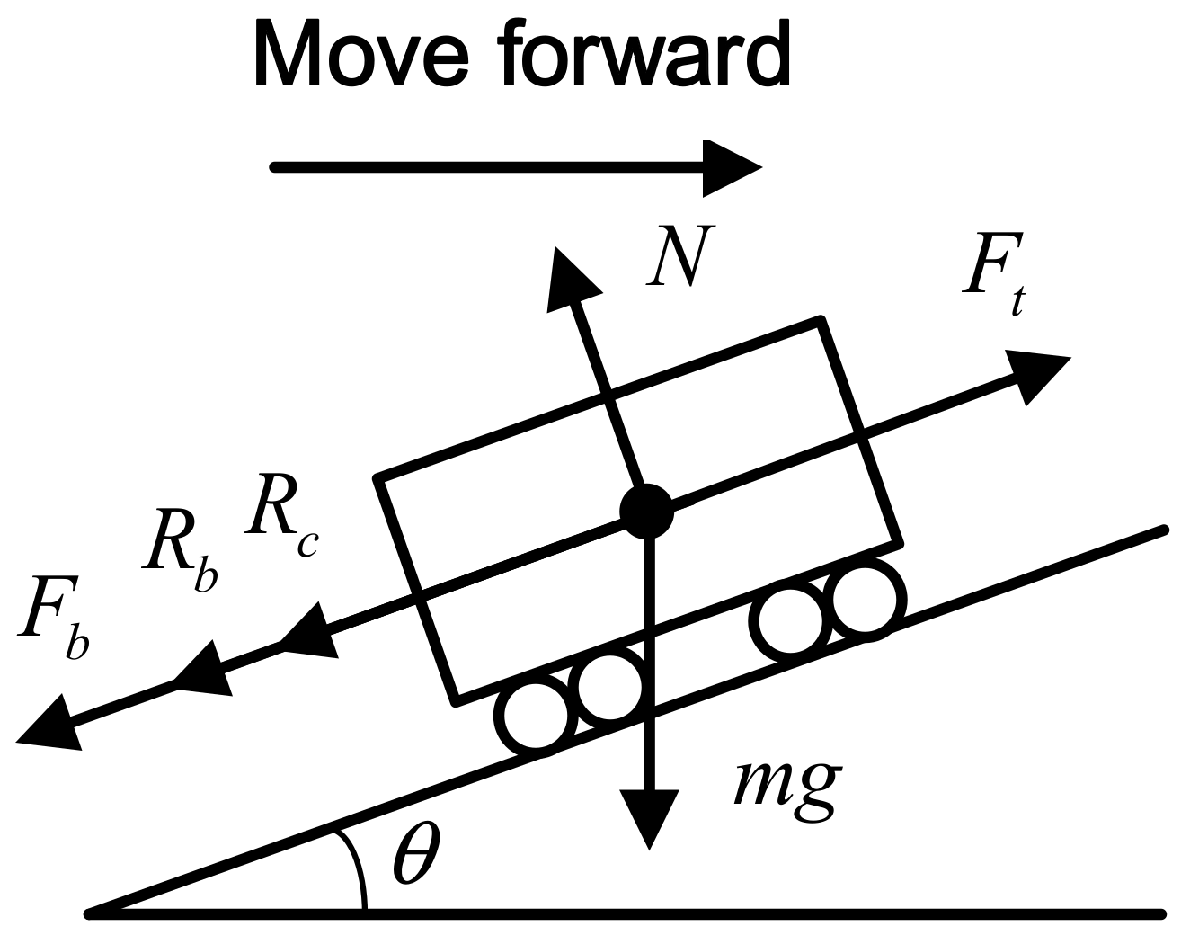
Train single-particle dynamics model in Reference [36] is used in this paper. The schematic diagram of the train force is shown in Figure 1. In this model, $m$ is the train mass, which is considered as a constant value throughout the journey. About the decomposition of the forces, denotes the traction force, $F_b$ denotes the braking force, $R_c$ denotes the additional resistance of the line that mainly comes from the slope, and $R_b$ denotes the basic running resistance of the train, mainly from the track and air. The dynamics model can be written as follows:

$$\begin{array}{c}\dot{x}=v\\ m\left(1+\gamma \right)\dot{v}=F_t\left(v\right)-F_b(v)-R_b\left(v\right)-R_c\left(v\right)\end{array}$$

(1)

where $v$ denotes the speed, and $x$ is the position; $F_t\left(v\right)$ is the force of traction, $F_b\left(v\right)$ is the force of braking, $R_c\left(v\right)$ is the additional resistance, and $R_b\left(v\right)$ is the basic resistance; and $\gamma$ is the rotary mass coefficient which is usually a given constant.

About the rotary mass coefficient, $\lambda$, it is a coefficient to compensate the moment of inertia. The train kinetic energy has two parts, one is the horizontal movement energy of the train, and the other is the moment of inertia of the wheels. Therefore, when only the horizontal movement is concerned, the moment of inertia needs to be compensated. This value can be obtained by dividing the converted weight of the moment of inertia by the total weight. Since this value is difficult to determine, empirical values are generally used in simulation. Therefore, $m\left(1+\gamma \right)$ is the total weight of the train after correction.

About the traction, the maximum that the train can provide is as follows:

$$F_{t\max }=\left\{\begin{array}{ll}203& 0\le v\le 51.5\\ -0.002v^3+0.49v^2-42.12v+1343& 51.5<v\le 90\end{array}\right.$$

(2)

$$F_t\left(v\right)={\mu }_t{F}_{t\max }\left(v\right),0<{\mu }_t<1$$

(3)

where $F_t(v)$ is the real force, and ${\mu }_t$ control factor.

About the braking, similar to traction, the calculation formula can be written as follows:

$$F_{b\max }=\left\{\begin{array}{ll}166& 0\le v\le 77\\ 0.134v^2-25.07v+1300& 77<v\le 90\end{array}\right.$$

(4)

$$F_b\left(v\right)={\mu }_b{F}_{b\max }\left(v\right),0<{\mu }_b<1$$

(5)

About the basic running resistance, it can be written as follows:

$$R_b\left(v\right)=r_1+r_{2}v+r_3{v}^2$$

(6)

where $r_1$, $r_2$, and $r_3$ are empirical parameters determined by experiment.

The additional resistance can be written as follows:

$$R_c\left(v\right)=w_i+w_r+w_s$$

(7)

where $w_i$ is the additional resistance of the slope, $w_r$ is the additional resistance in the curve, and $w_s$ is the additional resistance in the tunnel. Generally, the resistance in the curve and tunnel are not considered in the study and the slope resistance is given as:

$$w_i=mg\sin \theta$$

(8)

where $m$ is the train mass, $g$ is the acceleration of gravity, and $\theta$ is the slope value.

The external characteristic curves (max force) of train traction and braking force are shown in Figure 2, and Equations (2), (4), and (6) are examined by the actual experiment from Qingdao Metro Line 6.

3. Fitness Calculation Function about Speed Profile Optimization

This part establishes the optimization model of the profile, including the energy consumption calculation model, penalty function about punctuality, and comfortableness. These factors will be discussed separately below.

3.1. Energy Consumption Calculation Function

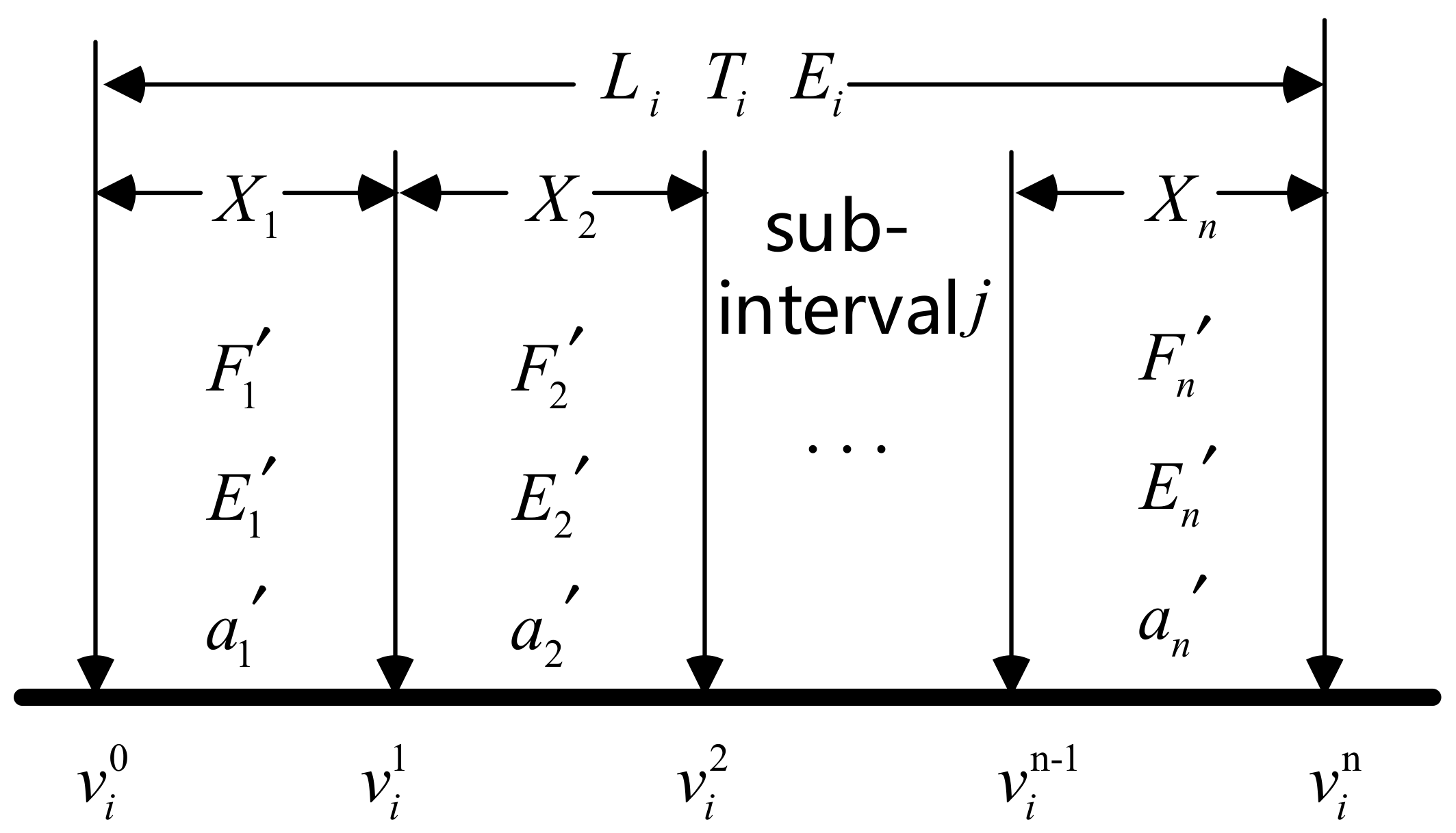
As shown in Figure 3, because of the speed limit, the operation of the metro on the entire line is divided into $N$ intervals, where $v_i^0\left(i=1,2,\mathrm{\dots },N\right)$ represents the starting speed of the train in the interval, $i$, and it also represents the ending speed in the interval, $i-1$; and $v_1^0$ and $v_{N+1}^0$ represent the starting speed and the arrival speed, respectively; obviously, $v_1^0=v_{N+1}^0=0$.

As shown in Figure 4, inside the interval, $i$, we split the single one into $n$ subintervals, which have same running time, $\Delta t$. In subinterval $n$, the description of the symbols is shown in

Table 1. Symbol description.

Symbol	Description
$F_n{}^{\prime }$	traction force
$E_n{}^{\prime }$	energy consumption
$a_n{}^{\prime }$	acceleration
$X_n$	length of the subinterval

.

Therefore, the length, $L_i$, and the time, $T_i$, of the interval,$i$, can be descripted as follows:

$$\begin{array}{l}{L}_i={\displaystyle \sum _{j=1}^n{X}_j}\\ T_i=n\cdot \Delta t\end{array}$$

(9)

The total length, $S_{total}$, and the total time, $T_{total}$, of all intervals are as follows:

$$\begin{array}{l}{S}_{total}={\displaystyle \sum _{i=1}^N{L}_i}\\ T_{total}={\displaystyle \sum _{i=1}^N{T}_i}\end{array}$$

(10)

The traction energy consumption, $E_j{}^{\prime }$, of subinterval can be calculated as follows:

$$E_j{}^{\prime }=F_j{}^{\prime }\cdot X_j$$

(11)

In Equation (11), the length of subinterval $X_j$ can be calculated as follows:

$$X_j=v_i^{j-1}\cdot \Delta t+0.5\cdot a_j{}^{\prime }\cdot \Delta t^2$$

(12)

Thus, the traction energy consumption of the interval, $i$, can be calculated as follows:

$$\begin{array}{l}E={\displaystyle \sum _{i=1}^N{E}_i}\\ E_i={\displaystyle \sum _{j=1}^n{E}_j{}^{\prime }}\end{array}$$

(13)

3.2. Punctuality Penalty Function

Punctuality is a key factor in evaluating the quality of metro operation. The current trains run on time according to the timetable issued by the ATS system. The running time between stations is already specified, and the error between the actual running time and the specified running time needs to be limited within a required error. According to the actual operation requirements of the metro, the maximum allowable time error is generally 6 s.

Define the punctuality judgment function of the train as follows:

$$T_{error}=\left|T_D-T_R\right|$$

(14)

where $T_{error}$ is the arrival time error, $T_D$ is the planned running time, and $T_R$ is the actual running time.

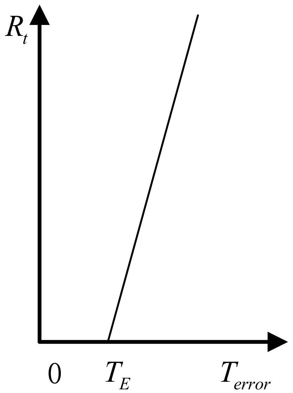
As shown in Figure 5, drawing on the Gaussian model, the punctuality penalty function is established as follows:

$$R_t=e^{\left(\frac{T_{error}-T_E}{{\rho }^2}\right)}$$

(15)

where $R_t$ is the time penalty factor, $T_E$ is the maximum allowable time error (set 6 s here), and $\rho$ is the sensitivity control coefficient, which can be used to control penalty level.

3.3. Comfortableness Penalty Function

Comfortableness is another important indicator of subway operation. Generally, the rate of change of acceleration is used to evaluate comfortableness.

Define the acceleration change rate calculation model as follows:

$$Jerk=\frac{da}{dt}$$

(16)

where $Jerk$ is the acceleration rate, $a$ is acceleration, and $t$ is running time.

As shown in Figure 6, similar to punctuality penalty function, the comfortableness penalty function is established as follows:

$$R_{com}=e^{\left(\frac{Jerk-J_d}{{\rho }^2}\right)}$$

(17)

where $R_{com}$ is comfortableness penalty factor, $J_d$ is maximum allowable acceleration rate of change, and $\rho$ is the sensitivity control coefficient.

As shown in

Table 2. International comfort standards.

Comfort Level	Acceleration Rate	Evaluation
Level 1	<0.315	Very comfortable
Level 2	0.315–0.63	Comfortable
Level 3	0.63–1.0	Relatively comfortable
Level 4	1.0–1.6	Uncomfortable
Level 5	1.6–2.5	Very uncomfortable
Level 6	>2.5	Extremely uncomfortable

, according to international standard IS02631 [38], set the value of $J_d$ to 1. When the acceleration change rate is larger, the penalty for comfort is greater, so that the non-conforming values in the result can be eliminated.

3.4. Fitness Calculation Function Based on Double Penalty Mechanism

As considered in Section 3.1, Section 3.2 and Section 3.3, the fitness calculation function based on double penalty mechanism is summarized as follows:

$$Min fitness=R_t+R_{com}+E$$

(18)

4. Speed Profile Optimization with RR-ABC

4.1. Emergency Braking Intervention (EBI) Curve and Warning Speed Limit

Resulted from some safety reasons, the metro line should consider various speed-limit protections.

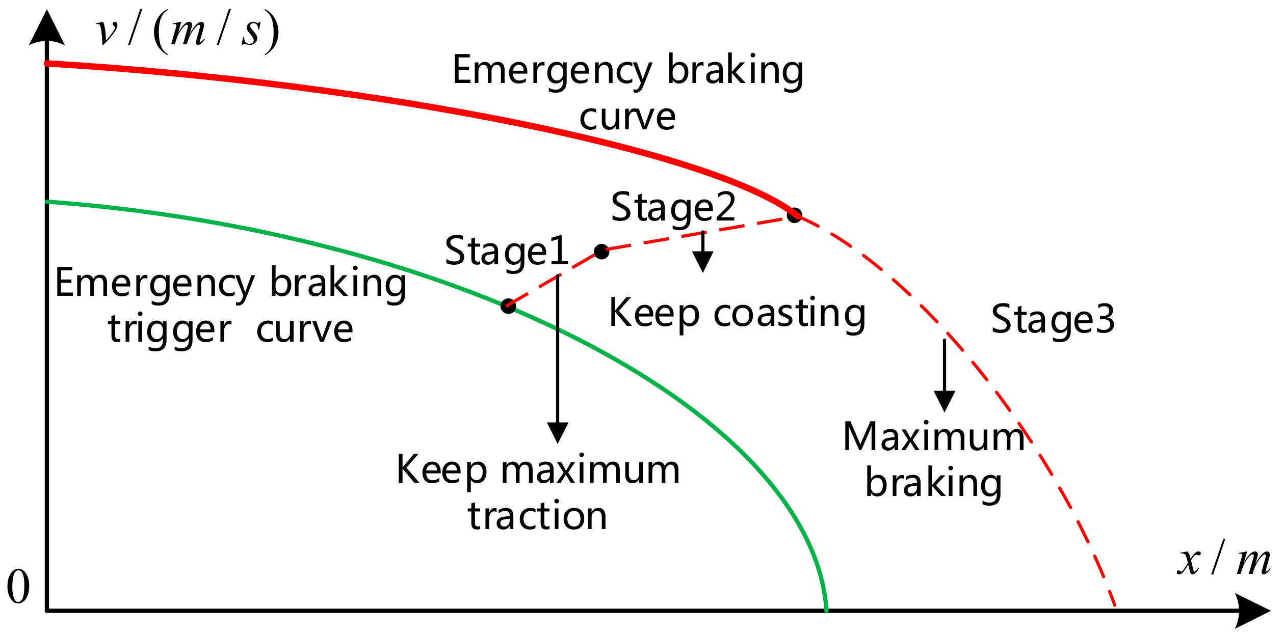
Firstly, the metro line has a fixed speed limit from the line. In addition, the metro also has a security protection mechanism to ensure that emergency braking is feasible in any position that the train cannot cross the fixed speed limit; this mechanism is called emergency braking intervention (EBI). To ensure that the metro does not exceed the fixed speed limit during emergency braking under any circumstances, the EBI protection considers such an extreme case:

• At first, the train is in the process of maximum acceleration. After the train issued an emergency braking command, the train still maintained the maximum acceleration during the transmission delay and traction cutoff delay, because the traction cannot be cut off instantly and transmission delay exists objectively at any moment.
• Since the braking system needs some time to receive instructions and gradually generate braking force, it usually takes some time to reach the maximum force from 0. During this period, the train is considered to keep coasting.

Therefore, as shown in Figure 7, the emergency braking process is divided into three stages:

Stage1: In this stage, the train accelerates with the maximum traction acceleration, and the acceleration time is the sum of the traction cutoff delay and the braking system action delay.

Stage2: After the train traction is cut off, the emergency braking force needs a certain time to reach the nominal value, and the train is considered to coast during this period.

Stage3: The train follows the emergency braking curve to brake.

Finally, as a result of the single-mass model, we ignore the size and length of the train. However, the ignorance will bring security risks to trains, so we design the warning speed limit based on the EBI curve.

As shown in Figure 8, when the train moves from the low-speed-limit zone to the high-speed-limit zone, the train needs to reserve a buffer equal to the length of the train. When the train moves from the high-speed-limit zone to the low-speed-limit zone, the same buffer is required.

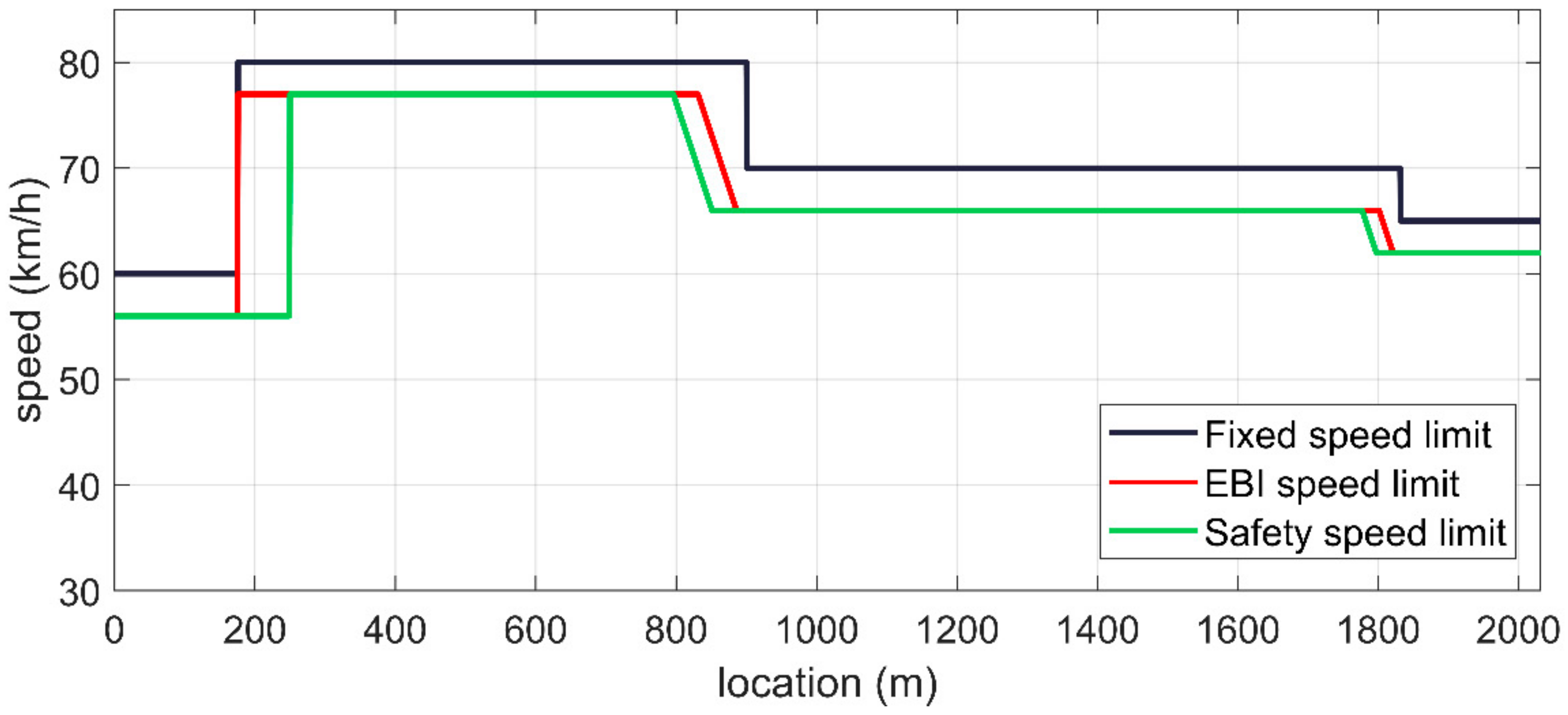
According to the above principle, taking Qingdao Metro Line 6 grabbing Zhuomashan station to Heluobu station as an example, these kinds of speed limit curves are obtained as shown in Figure 9.

4.2. Energy-Saving Strategies and Coast Choices

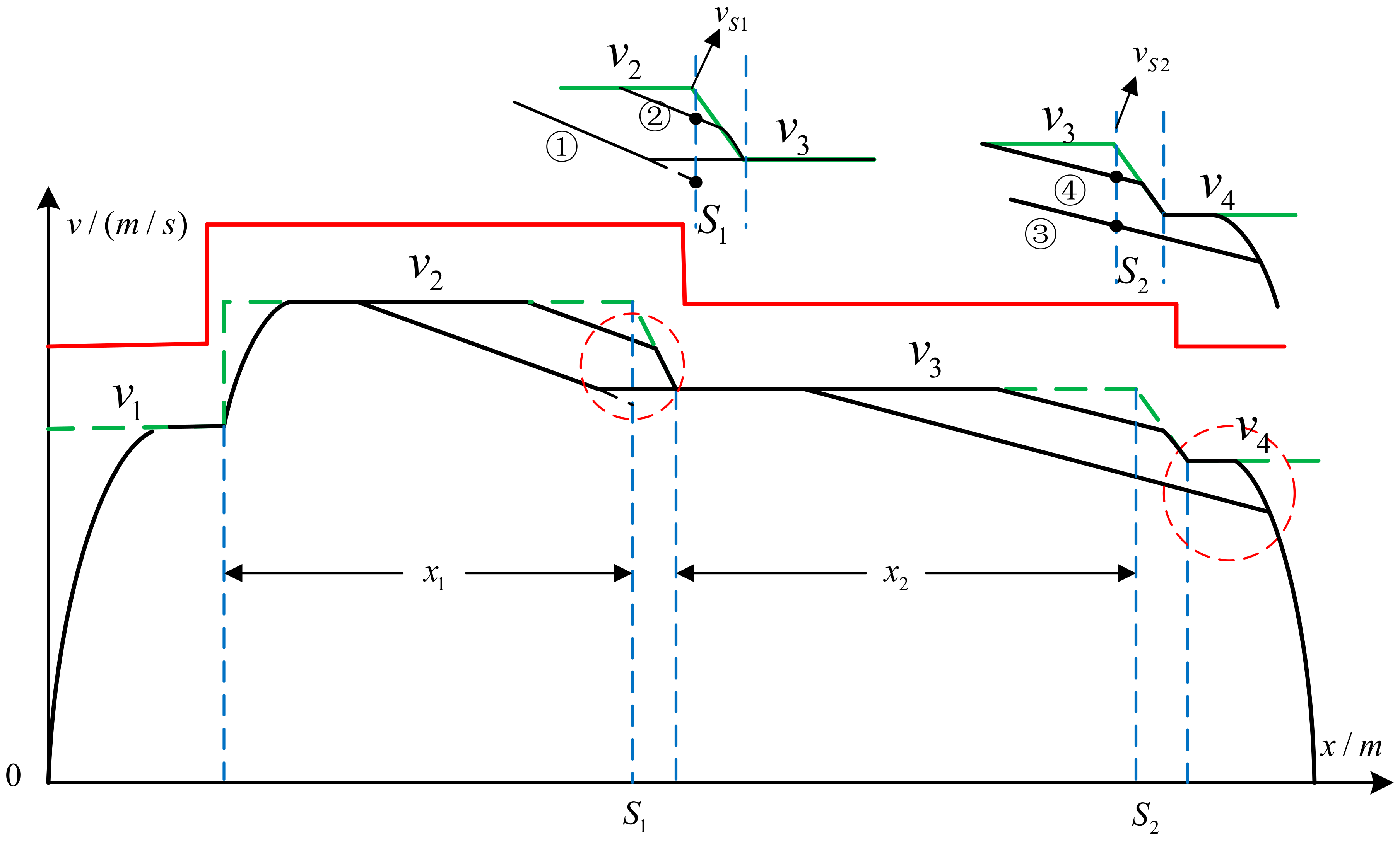
According to actual operating conditions and theory, coast travel is an effective strategy for train energy saving. The coast strategy we designed is shown in the Figure 10, in which two different coast intervals are set.

4.2.1. Coast Interval $x_1$

• Features:

  (1)

  Driving from high speed limit zone to low speed limit zone

  (2)

  Maintain constant speed at the next low speed limit

• Strategy selection:

From the coast point, let the train maintain the coast condition until point $S_1$, then we get the speed of $S_1$ point $v_{S1}$.

(1)

If $v_{S1}>v_3$, then brake to $v_3$;

(2)

If $v_{S1}<v_3$, then when $v=v_3$, let the train drive at a constant speed $v_3$.

4.2.2. Coast Interval $x_2$

• Features:

  (1)

  Driving from high speed limit zone to low speed limit zone;

  (2)

  Braking in the next low speed limit.

• Strategy selection:

From the coast point, let the train maintain the coast condition until point $S_2$, then we get the speed of $S_2$ point $v_{S2}$.

(1)

If $v_{S2}>v_4$, then brake to $v_4$;

(2)

If $v_{S2}\le v_4$, then keep coasting to maintain the coast condition until it contacts the braking curve.

4.3. Regional Reinforcement Artificial Bee Colony (RR-ABC) Algorithm

The ABC algorithm simulates the process of the bee colony searching for the honey source with the highest honey content. It has few control parameters, and it has good global convergence. However, when the local search is approached to converge to the optimal solution, the search efficiency drops sharply [39,40]. With the deepening of evolution, population diversity is seriously lacking, and the search efficiency is significantly reduced at the end of evolution. To balance the global and local search capabilities and to improve efficiency of the ABC, a more efficient ABC algorithm is proposed called RR-ABC algorithm. The principles and steps of the RR-ABC algorithm are as follows:

(1) 

Model initialization: Chaos mirror initialization

Because of the randomness of the chaotic map and the sensitivity to the initial conditions, we extracted the decision space information to grow the diversity of the group. In this part, the sine formula is used to iteratively generate chaotic variables. The chaotic initialization Equation is as follows:

$$\begin{array}{c}c{h}_1=rand\left(0,1\right)\\ c{h}_{k+1}=\sin \left(\pi c{h}_k\right)\\ x_{ij}=x_{ij\min }+c{h}_{kj}\left(x_{ij\max }-x_{ij\min }\right)\end{array}$$

(19)

where $c{h}_1$ is random number between 0 and 1; $k$ is number of iterations; $k=1,2,\mathrm{\dots },D-1$, and $j=1,2,\mathrm{\dots },D$; $x_{ij}$ is the j-dimensional parameter of the i-th honey source; and $x_{ij\max }$,$x_{ij\min }$ are the top and bottom limits of the source.

Use Equation (19) to perform the chaos initialization operation to obtain the $i-\mathrm{th}$ honey source $x_i=(x_{i1},x_{i2},\mathrm{\dots },x_{iD})$, then mirror it to get the mirror honey source $mi{r}_i=\left(x_{iD},\mathrm{\dots },x_{i2},x_{i1}\right)$, then compare the fitness value of the initial solution one by one, and select the better individual as the initial population.

(2) 

Employed bee stage: Evolutionary dimension adjustment strategy

In the stage of employed bee and onlooker bee, they need to update the honey source through Equation (20); the original honey source has only one dimension for each change. Obviously, this method is extremely inefficient. To solve the problem, we use a new parameter $W$, to control the dimensions that need to be changed in each evolution. The new search Equation is as follows:

$$x_{iw}{}^{\prime }=x_{iw}+R_{iw}\times \left(x_{iw}-x_{kw}\right)$$

(20)

where $w=\left\{1,2,\mathrm{\dots },W\right\}$, parameter $W$ controls the number of dimensions of each individual change, and $W=\left\{1,2,\mathrm{\dots },D\right\}$.

Every time an employed bee searches for a new honey source, it will estimate the potential of the source (calculate the fitness value of the objective function):

$$fit=\frac{1}{1+f_i}$$

(21)

where $f_i$ is the objective function value of the i-th honey source; $fi{t}_i$ is the fitness value of i-th honey source. The employed bee chooses the better honey source by comparing the fitness value of $X_i$ and $X_i{}^{\prime }$ (Greedy choice). The larger the fitness value, the smaller the corresponding objective function value, indicating that the honey source is also better, and with a higher probability of getting better honey sources around it.

$$X_i{}^{\prime }=\left\{\begin{array}{l}{X}_i{}^{\prime } fit(X_i{}^{\prime })>fit(X_i)\\ X_i fit(X_i{}^{\prime })\le fit(X_i)\end{array}\right.$$

(22)

(3) 

Onlooker bees stage: Search radius adjustment strategy

As mentioned in “Model of employed bees”, the employed bee will search within a certain radius of the initial solution. In the early stage of evolution, because the honey source $x_i$ is far from the real solution, the use of a larger search radius can accelerate the convergence rate; when the honey source evolves to the final stage, it is closer to the real solution, and reducing the search radius can improve the search accuracy. Therefore, using a variable search radius and adjusting the size of the search radius can significantly speed up the convergence rate.

In this paper, the strategy of changing the search radius with the individual threshold, that is, as the threshold, $Limi{t}_i{}^{\prime }$ (the digit of times that honey source $x_i$ was not selected), increases, the search radius continues to decrease. The Equation is as follows:

$$r_{iw}=\varphi +\cos \left(\frac{\pi Limi{t^{\prime }}_{iw}}{2Limit}\right)$$

(23)

where $r_{iw}$ is search radius honey source $x_{iw}$, $\varphi$ is the basic value of search radius, $Limi{t}_{iw}{}^{\prime }$ is the threshold of the honey source $x_{iw}$, and $Limit$ is the maximum allowed threshold. The new search Equation is as follows:

$$x_{iw}{}^{\prime }=x_{iw}+r_{iw}\times \left(x_{iw}-x_{kw}\right)$$

(24)

Remark 1.

For the traditional ABC algorithm, with the deepening of evolution, more nectar sources are continuously explored on a global scale. However, due to the unknown quality of the preliminary search results, each explored nectar needs to be searched more deeply, which seriously affects the search efficiency in the later stages of evolution, even if it can avoid the generation of local optimal solutions. In addition, for classic biomimetic algorithms, the quality of the initial value usually greatly affects the evolution process, while a simple random process can easily produce low-quality initial values. Through the flowchart about the comparison of classic method and reinforcement method (Figure 11), we can see that dynamically adjusted evolutionary dimensions and search radius are adopted. In the later stages of the search, fewer high-quality nectar sources will be paid attention, and a better efficiency can be got.

4.4. Speed Profile Optimization Model

Based on the above discussion, the speed curve optimization model is summarized as follows:

$$Min fitness=E+R_t+R_{com}$$

(25)

s.t.

$$\left\{\begin{array}{l}\dot{x}=v\\ m\left(1+\gamma \right)\dot{v}=F_t\left(v\right)-F_b\left(v\right)-R_b\left(v\right)-R_c\left(v\right)\\ 0\le v\le v_{safety}\end{array}\right.$$

(26)

5. Adaptive Terminal Sliding Mode Controller

This section needs to design a speed tracking controller to track the speed profile optimized before. As mentioned before, compared with PID controller, which is widely used in modern industrial control, the sliding mode controller is quick to respond and completely robust to system parameter changes and external interference. However, sliding mode control will produce chattering when dealing with uncertain factors. This kind of high-frequency chattering will not only affect the accuracy of the control, but also cause the system to oscillate or become unstable.

Adaptive terminal sliding mode control not only has strong robustness, but also lets the system state converge to the ideal trajectory within a limited time. In addition, it also has a strong parameter adaptive processing function, to ensure that the system will not have unnecessary continuous switching when the parameters are uncertain. In order to design a speed-tracking controller with excellent comprehensive performance, this paper designs an adaptive terminal sliding mode controller with disturbance observer.

5.1. Dynamics Model of Speed Tracking

This part models and transforms the known fixed time delay. Here, the time delay is compensated by the sliding mode control coefficient, so that the system can be used as a non-delay system to design the sliding mode control rate in the subsequent chapters.

As mentioned in Section 2, the ideal dynamics model is Equation (1); for convenience of expression, the model with speed $v$ as its independent variable is rewritten as the model with time, $t$, as its independent variable. Furthermore, the traction force factor, $F_t\left(v\right)$, and braking force factor,$F_b\left(v\right)$, are replaced by the actual generated traction/braking force, $F_u\left(t\right)$, and the model is summarized as follows:

$$\left\{\begin{array}{l}\dot{x}=v\\ m\left(1+\gamma \right)\dot{v}=F_u\left(t\right)-R_b\left(t\right)-R_c\left(t\right)\end{array}\right.$$

(27)

In the actual control system, due to response delay, the model needs to be written as a first-order lag model:

$${\dot{a}}_c\left(t\right)=-\frac{1}{\tau }{a}_c\left(t\right)+\frac{1}{\tau }{a}_t\left(t-T_d\right)$$

(28)

where $a_c$ is the control acceleration, which is produced by the controller; $a_t$ is the target acceleration; $\tau$ is the response time constant; and $T_d$ is controlling transmission delay.

For subsequent kinetic description, we define the following Equation:

$$a_c=\frac{F_u\left(t\right)}{m\left(1+\gamma \right)}$$

(29)

Therefore, the acceleration formed by the basic resistance of the train and the additional resistance can be expressed as follows:

$$\begin{array}{c}d\left(t\right)=-W\left(t\right)-a-bv-c{v}^2\\ W\left(t\right)=\frac{R_a\left(t\right)}{m\left(1+\gamma \right)}\\ a=\frac{r_1}{1+\gamma }\\ b=\frac{r_2}{1+\gamma }\\ c=\frac{r_3}{1+\gamma }\end{array}$$

(30)

Furthermore, according to Equation (30), we can get the following:

$$\dot{v}\left(t\right)=a_c\left(t\right)+d\left(t\right)$$

(31)

where $d\left(t\right)$ is the resistance acceleration.

The existing metro controllers are mostly stepless control modes, and the control system model is shown in Figure 12.

In order to facilitate the design of subsequent controllers, pade approximation is used to rewrite the delay parameters $T_d$, in Equation (28):

$$e^{-T_{d}s}\approx \frac{-s+\lambda }{s+\lambda }$$

(32)

where $\lambda$ is a constant related to delay, $T_d$.

Laplace transform of Equation (28):

$$a_c=-\frac{\tau }{\lambda }{\ddot{a}}_c-\frac{\lambda \tau +1}{\lambda }{\dot{a}}_c-\frac{1}{\lambda }{\dot{a}}_t+a_t$$

(33)

In order to facilitate expression, Equation (33) is rewritten as follows:

$$\begin{array}{c}{a}_c=-q_1{\ddot{a}}_c-q_2{\dot{a}}_c-q_3{\dot{a}}_t+a_t\\ q_1=\frac{\tau }{\lambda }\\ q_2=\frac{\lambda \tau +1}{\lambda }\\ q_3=\frac{1}{\lambda }\end{array}$$

(34)

As we can see, if the response time constant $\tau$ and the delay $T_d$ are known and kept unchanged, then $q_1$, $q_2$, and $q_3$ are all constants. In the following content $q_1$,$q_2$, and $q_3$ are used to design the sliding mode control rate, so the delay will be compensated. The time delay is compensated to the sliding mode control rate coefficient through the abovementioned method, and the effect of delay is eliminated in this way.

5.2. Design of Sliding Mode Terminal Controller

We define the state error as follows:

$$\left\{\begin{array}{l}{e}_1=x-x_r\\ e_2=v-v_r\end{array}\right.$$

(35)

where $e_1$ is the train position error, $e_2$ is the train speed error, $x_r$ is the reference position of optimized profile, and $v_r$ is the reference speed of optimized profile.

Differentiate Equation (35) and substitute it into Equation (31), and the resulting error state space Equation is as follows:

$$\left\{\begin{array}{l}{\dot{e}}_1=e_2\\ {\dot{e}}_2=a_c+d-{\dot{v}}_r\end{array}\right.$$

(36)

To improve the tracking accuracy, the designed sliding mode surface needs to introduce the train position error $e_1$, and speed error $e_2$, to ensure fast error convergence. The designed terminal sliding mode function is as follows:

$$s_m\left(t\right)=\beta e_1+e^{p/q}{}_2$$

(37)

where $\beta >0$; and $p$ and $q$ are positive odds,$1<\frac{p}{q}<2$.

Design the sliding mode controller below.

Differentiate the sliding mode function of (37) as follows:

$${\dot{s}}_m\left(t\right)=\beta e_2+\frac{p}{q}\left(a_c+d-{\dot{v}}_r\right)e_2^{p/q-1}$$

(38)

According to Equations (30) and (31), we can obtain the following:

$$\left\{\begin{array}{l}{a}_c=\dot{v}+a+bv+c{v}^2+W\left(t\right)\\ {\dot{a}}_c=\ddot{v}+b\dot{v}+2cv\dot{v}+\dot{W}\left(t\right)\\ {\ddot{a}}_c=\stackrel{⃛}{v}+b\ddot{v}+2cv\ddot{v}+2c{\dot{v}}^2+\ddot{W}\left(t\right)\end{array}\right.$$

(39)

Substitute Equation (39) into Equation (34), since $q_{1}b\ll q_2$, ignore $q_{1}b\ddot{v}$, and get the following:

$$a_c=-q_1\left(\stackrel{⃛}{v}+2c{\dot{v}}^2+2cv\ddot{v}+W\left(t\right)\right)-q_2\left(\ddot{v}+b\dot{v}+2cv\dot{v}+\dot{W}\left(t\right)\right)-q_3{\dot{a}}_t+a_t$$

(40)

By combining Equations (39) and (40), and bringing Equation (40) into the first derivative (38) of the sliding mode function, we can obtain the following:

$$\begin{array}{l}{\dot{s}}_m\left(t\right)=\beta e_2+\frac{p}{q}{e}_2^{p/q-1}\left(-a-bv-c{v}^2-W\left(t\right)-q_1\ddot{W}\left(t\right)-q_2\dot{W}\left(t\right)-{\dot{v}}_r\right)\\ +\frac{p}{q}{e}_2^{p/q-1}\left(-q_1\stackrel{⃛}{v}-2q_{1}c{\dot{v}}^2-2q_{1}cv\ddot{v}-q_2\ddot{v}-q_{2}b\dot{v}-2q_{2}cv\dot{v}-q_3{\dot{a}}_t+a_t\right)\end{array}$$

(41)

Based on the principle of sliding mode controller, the sliding mode control input has the following form:

$$u\left(t\right)=u_{eq}+u_n$$

(42)

where $u_{eq}$ is the equivalent control items of the system, and $u_n$ is the nonlinear switching control items of the system.

Make Equation (41) approach zero, to get the following:

$$\begin{array}{l}{u}_{eq}=-\frac{q}{p}\beta e_2^{2-p/q}+W\left(t\right)+q_1\ddot{W}\left(t\right)+q_2\dot{W}\left(t\right)+a+bv+c{v}^2\\ +{\dot{v}}_r+q_1\stackrel{⃛}{v}+2q_{1}c{\dot{v}}^2+2q_{1}cv\ddot{v}+q_2\ddot{v}+q_{2}b\dot{v}+2q_{2}cv\dot{v}+q_3{\dot{a}}_t\end{array}$$

(43)

Make $D\left(t\right)=\left(-W\left(t\right)-q_1\ddot{W}\left(t\right)-q_2\dot{W}\left(t\right)-a-bv-c{v}^2\right)$, since $W\left(t\right)$ is a smooth resistance and has a boundary; then its first and second derivatives are bounded, and the basic running resistance of the train $f_b\left(t\right)$ is bounded, so there is $D\le D_{\max }$, and $D_{\max }$ is the boundary. According to the design principle of sliding mode control, the nonlinear switching term is designed as $u_n=-k\mathrm{sgn}\left(s_m\right)$, and then the terminal sliding mode control input is as follows:

$$\begin{array}{l}u\left(t\right)=-\frac{q}{p}\beta e_2^{2-p/q}+q_1\stackrel{⃛}{v}+q_2\ddot{v}+q_3{\dot{a}}_t+2q_{1}c{\dot{v}}^2+2q_{1}cv\ddot{v}\\ +q_{2}b\dot{v}+2q_{2}cv\dot{v}-D+{\dot{v}}_r-k\mathrm{sgn}\left(s_m\right)\end{array}$$

(44)

where $k>0$ is the control gain.

In addition, since the resistance items of the train are unknown in the actual operation of the train, that is $D$ is unknown, but $D$ is bounded, the actual controller should be changed to the following:

$$\begin{array}{l}u\left(t\right)=-\frac{q}{p}\beta e_2^{2-p/q}+q_1\stackrel{⃛}{v}+q_2\ddot{v}+q_3{\dot{a}}_t+q_4{\dot{v}}^2\\ +2q_{4}v\ddot{v}+q_5\dot{v}+2q_{6}v\dot{v}+{\dot{v}}_r-k\mathrm{sgn}\left(s_m\right)\end{array}$$

(45)

where $q_4=q_{1}c$; $q_5=q_{2}b$; $q_6=q_{2}c$; and $k>D_{\max }$.

Select the Lyapunov function of the following form:

$$V\left(t,x\right)=\frac{1}{2}{s}_m^2\left(x\right)$$

(46)

Let $k_0=k-D_{\max }$, derivate Equation (46), and bring the controller formula, Equation (45), into it:

$$\begin{array}{l}\dot{V}=s_m{\dot{s}}_m=s_m\left(-k_0\frac{p}{q}\mathrm{sgn}(s_m)-\frac{p}{q}\left(D_{\max }\mathrm{sgn}(s_m)-D\right)\right)e_2^{p/q-1}\\ \le \left(-k_0\frac{p}{q}{e}_2^{p/q-1}\right)\left|s_m\right|<0\\ \end{array}$$

(47)

The system is stable, but in order to reduce the control burden of switching items and reduce the possibility of chattering, a parameter adaptation mechanism is introduced.

First modify the controller to the following form:

$$\begin{array}{l}u\left(t\right)=-\frac{q}{p}\beta e_2^{2-p/q}+{\widehat{q}}_1\stackrel{⃛}{v}+{\widehat{q}}_2\ddot{v}+{\widehat{q}}_3{\dot{a}}_t+2{\widehat{q}}_4{\dot{v}}^2\\ +2{\widehat{q}}_{4}v\ddot{v}+{\widehat{q}}_5\dot{v}+2{\widehat{q}}_{6}v\dot{v}+\widehat{a}+\widehat{b}v+\widehat{c}{v}^2+{\dot{v}}_r-k\mathrm{sgn}\left(s_m\right)\end{array}$$

(48)

where ${\widehat{q}}_1,{\widehat{q}}_2,{\widehat{q}}_3,{\widehat{q}}_4,{\widehat{q}}_5,{\widehat{q}}_6,\widehat{a},\widehat{b},\widehat{c}$ are the estimated values of parameters $q_1,q_2,q_3,q_4,q_5,q_6$$a,b,c$, respectively.

Construct the following Lyapunov function:

$$\dot{V}=s_m{\dot{s}}_m+{\displaystyle \sum _{i=1}^6\frac{1}{{\lambda }_i}\Delta q_i\Delta {\dot{q}}_i}+\frac{1}{{\lambda }_7}\Delta a\Delta \dot{a}+\frac{1}{{\lambda }_8}\Delta b\Delta \dot{b}+\frac{1}{{\lambda }_9}\Delta c\Delta \dot{c}$$

(49)

where

$$\left\{\begin{array}{l}\Delta a=\widehat{a}-a,\Delta \dot{a}=\dot{\widehat{a}}\\ \Delta b=\widehat{b}-b,\Delta \dot{b}=\dot{\widehat{b}}\\ \Delta c=\widehat{c}-c,\Delta \dot{c}=\dot{\widehat{c}}\\ \Delta q_i={\widehat{q}}_i-q_i,\Delta {\dot{q}}_i={\dot{\widehat{q}}}_i i=1,2,\cdots ,6\end{array}\right.$$

Bring Equation (48) into Equation (49), and we can get the following:

$$\begin{array}{cc}\hfill & \dot{V}=\frac{p}{q}{e}_2^{p/q-1}\left(\left({\widehat{q}}_1-q_1\right)+\ddot{v}\left({\widehat{q}}_2-q_2\right)+{\dot{a}}_t\left({\widehat{q}}_3-q_3\right)\right)s_m\hfill \\ \hfill & +\frac{p}{q}{e}_2^{p/q-1}\left(2{\dot{v}}^2\left({\widehat{q}}_4-q_4\right)+2v\ddot{v}\left({\widehat{q}}_4-q_4\right)+\dot{v}\left({\widehat{q}}_5-q_5\right)\right)s_m\hfill \\ \hfill & +\frac{p}{q}{e}_2^{p/q-1}\left(2v{\dot{v}}^2\left({\widehat{q}}_6-q_6\right)+\left(\widehat{a}-a\right)+v\left(\widehat{b}-b\right)+s_m\left(\widehat{c}-c\right)\right)\hfill \\ \hfill & -\frac{p}{q}{e}_2^{p/q-1}{s}_m\left(k+G_{max}\right)\left(s_m\right)\hfill \\ \hfill & +\sum _{i=1}^6\frac{1}{{\lambda }_i}\Delta q_i\Delta {\dot{q}}_i+\frac{1}{{\lambda }_7}\Delta a\Delta \dot{a}+\frac{1}{{\lambda }_8}\Delta b\Delta \dot{b}+\frac{1}{{\lambda }_9}\Delta c\Delta \dot{c}\hfill \end{array}$$

(50)

To meet the stability rules of the Lyapunov formula, organize Equation (50), and the available parameter adaptation law is as follows:

$$\left\{\begin{array}{c}{\dot{\widehat{q}}}_1=-{\lambda }_1\frac{p}{q}{e}_2^{p/q-1}{s}_m,{\dot{\widehat{q}}}_2=-{\lambda }_2\frac{p}{q}{e}_2^{p/q-1}{s}_m\ddot{v}\hfill \\ {\dot{\widehat{q}}}_3=-{\lambda }_3\frac{p}{q}{e}_2^{p/q-1}{s}_m{\dot{a}}_1,{\dot{\widehat{q}}}_4=-{\lambda }_4\frac{p}{q}{e}_2^{p/q-1}{s}_m\left({\dot{v}}^2+v\ddot{v}\right)\hfill \\ {\dot{\widehat{q}}}_5=-{\lambda }_5\frac{p}{q}{e}_2^{p/q-1}{s}_m\dot{v},{\dot{\widehat{q}}}_6=-2{\lambda }_6\frac{p}{q}{e}_2^{p/q-1}{s}_{m}v\dot{v}\hfill \\ \dot{\widehat{a}}=-{\lambda }_7\frac{p}{q}{e}_2^{p/q-1}{s}_m\hfill \\ \dot{\widehat{b}}=-{\lambda }_8\frac{p}{q}{e}_2^{p/q-1}{s}_{m}v\hfill \\ \dot{\widehat{c}}=-{\lambda }_9\frac{p}{q}{e}_2^{p/q-1}{s}_m{v}^2\hfill \end{array}\right.$$

(51)

As showed in Equations (50) and (51), discontinuous switching function $k\mathrm{sgn}(s_m)$, will result in unconnected control signals to keep the train running on the sliding surface. However, due to resistance deviation, measurement deviation, and other factors, the train cannot stay on the sliding surface, which will eventually cause chattering. To avoid chattering, replace signum function $\mathrm{sgn}(s_m)$, in Equation (47) with saturation function, $sat(s_m)$ and $\varphi$ is the saturation width.

Generally speaking, the distinguishing feature of typical sliding mode control is the use of a signum function. After the introduction of a saturation function, the controller will no longer be a classic sliding mode controller. According to References [41,42], the sat function implies a pseudo sliding mode in fact.

$$sat(s_m)=\left\{\begin{array}{l}1 s_m>\varphi \\ s_m \left|s_m\right|\le \varphi \\ -1 s_m<-\varphi \end{array}\right.$$

(52)

5.3. Disturbance Observer

The introduction of the saturation function will reduce the robustness of the system, but the line interference may be greater during train operation, especially on ramps. Disturbance observer (DOB) has been one of the most widely used robust control tools which can effectively improve robustness and anti-disturbance [43,44]. Therefore, a disturbance observer is introduced in this part.

The Equation (48) is introduced into the disturbance observation value and transformed into the following form:

$$u\left(t\right)=-\frac{q}{p}\beta e_2^{2-p/q}+{\widehat{q}}_1\stackrel{⃛}{v}+{\widehat{q}}_2\ddot{v}+{\widehat{q}}_3{\dot{a}}_t-\widehat{d}-{\widehat{q}}_1\widehat{d}+{\dot{v}}_r-k\mathrm{sgn}\left(s_m\right)$$

(53)

As shown in Figure 13, the actual model and the nominal model are as follows:

$$\left\{\begin{array}{l}G=\frac{e^{-T_{d^s}}}{\tau s+1}\\ G_n=\frac{e^{-T_{n^s}}}{{\tau }_{n^S}+1}\end{array}\right.$$

(54)

According to the principle of disturbance observer, by considering the input term as the transfer function of $u_r$ and $d$, we can get the following:

$$\begin{array}{l}{G}_{d\widehat{d}}\left(s\right)=\frac{\widehat{d}}{d}=\frac{Q\left(s\right)}{1+Q\left(s\right)G\left(s\right)-G_n\left(s\right)Q\left(s\right)}\\ G_{u_r\widehat{d}}\left(s\right)=\frac{\widehat{d}}{u_r}=\frac{G\left(s\right)Q\left(s\right)-G_n\left(s\right)Q\left(s\right)}{1+G\left(s\right)Q\left(s\right)-G_n\left(s\right)Q\left(s\right)}\end{array}$$

(55)

Furthermore, the expression of the disturbance observation can be obtained as follows:

$$\widehat{d}=G_{u_r\widehat{d}}\left(s\right)u_r+G_{d\widehat{d}}\left(s\right)d$$

(56)

According to Equation (56), if $G_n\left(s\right)=G\left(s\right)$, the required disturbance value can be accurately observed, but in the actual system, there may be a deviation between $G_n\left(s\right)$ and $G\left(s\right)$. From Equation (56), the deviation of the estimated value mainly comes from the error of the model:

$$\Delta \widehat{d}=\frac{\Delta G\left(s\right)\left(d-u_r\right)}{1-\Delta G\left(s\right)}$$

(57)

where $\Delta G\left(s\right)=G_n\left(s\right)-G\left(s\right)$, $Q\left(s\right)$ is the low pass filter, and $Q\left(s\right)=1$.

According to Equation (57), if there is an error in the model, the obtained observations will also have a certain deviation. The magnitude of the model error determines the magnitude of the deviation of the observations. After introducing the disturbance observer, the gain of the switching function will be weakened to a certain extent. In general, the error of the train model is small, so the disturbance observer can improve the anti-interference ability of the system and reduce the switching gain, to avoid chattering.

6. Experimental Result

To verify the validity, this section uses the interval between Zhuomashan station and Heluobu station in Qingdao Metro Line 6 as the simulation object.

6.1. Basic Test of RR-ABC

The vehicle data and line data (slope and speed limit) used are shown in

Table 3. Vehicle data.

Vehicle Parameters	Evaluation
Formation	6 trains
Mass-AW2 (ton)	339.6
Length (m)	120
Basic resistance parameters ($r_1$)	9.067
Basic resistance parameters ($r_2$)	0
Basic resistance parameters ($r_3$)	0.001334

,

Table 4. Ramp data.

Location (m)	Slope (‰)
0–97	0
97–377	2.357
377–1087	10
1087–1926	17.682
1926–2045	0

, and

Table 5. Speed-limit data.

Location (m)	Speed Limit (km/h)
0–175	60
175–900	80
900–1831	70
1831–2030	65

, respectively.

To verify the effectiveness of the AA-ABC algorithm, we compare it with the standard ABC algorithm and the GA, respectively. We set the given interval running time to 147 s and use different evolutionary algorithms for testing. For each algorithm, we conducted three repeated experiments. The results are shown in Figure 13.

Figure 14a is the comparison of the RR-ABC algorithm and the standard ABC algorithm; the line in the figure represents the changing trend of fitness. We can observe the following two results:

(1)

The initial value of the RR-ABC algorithm is better than that of the standard ABC algorithm;

(2)

Compared with the standard ABC algorithm, RR-ABC maintained good evolutionary performance, both in the early and late stages; especially in the late stage, the evolution efficiency of RR-ABC is significantly higher than that of ABC. This proves that the RR-ABC algorithm has good local search capabilities.

Figure 14b is the comparison of the RR-ABC algorithm and GA; we can observe that GA gets a local optimal solution twice. Relatively speaking, ABC has good global search capabilities

By combining Figure 14a,b, we can find that RR-ABC algorithm has better global search capabilities compared with ordinary evolutionary algorithms. Furthermore, it also improves the local search capabilities, which are poor in standard ABC algorithm. RR-ABC algorithm can quickly obtain the optimal solution.

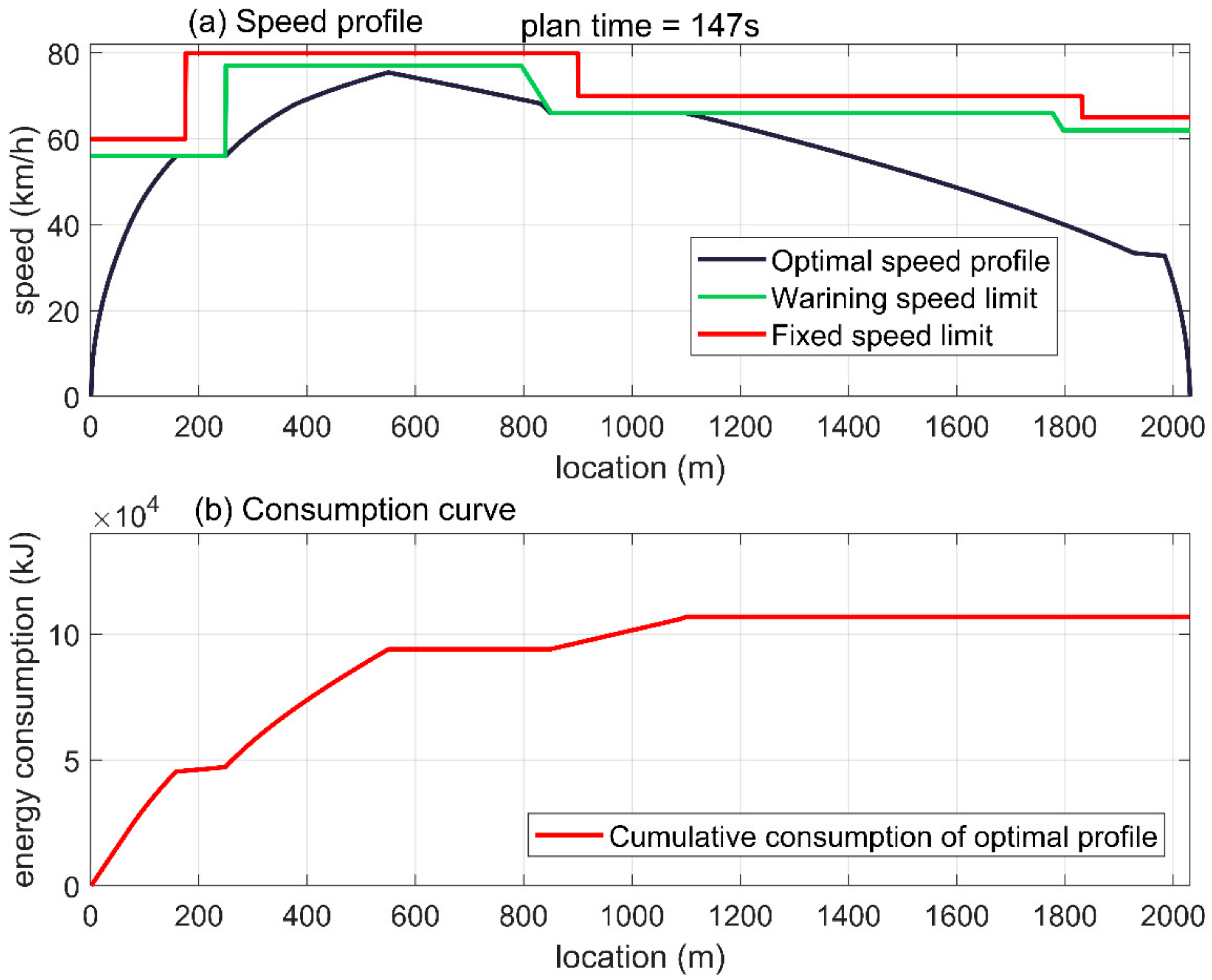
Figure 15a is the optimal speed profile, and Figure 15b is the energy-consumption curve. Figure 15a shows the fixed speed limit curve, the economic speed limit curve, and the optimal speed curve. The curve in Figure 15b shows the cumulative upward trend of energy consumed by the train as the vehicle moves. We can observe the following results:

(1)

Running with the safety speed limit curve, the train can safely travel under the fixed speed limit curve;

(2)

The speed profile contains two coast sections;

(3)

When the train is in traction section and cruising section, the energy consumption increases. Furthermore, the rate during traction is higher than that in cruise. In contrast, the energy consumption remains a level-out during coast section and braking section.

6.2. Advanced Test about Different Interval Time and Different Mode

To verify the performance of the algorithm under different running times, set the given interval time to 141 and 153 s, respectively. The results are shown in Figure 16 and Figure 17.

In Figure 16, because of the reduction of running time, compared with the speed profile shown in Figure 15, we can observe that coast sections are shortened and the energy consumption is higher. In Figure 17, resulted from the growth of running time, we can observe that coast sections are extended and the energy consumption is lower.

The detailed data of the comparison are shown in

Table 6. Detailed data for comparison.

Given Time (s)	Real Time (s)	Consumption (kJ)	Average Acceleration Rate (m/s3)
141	143.6	118,147	0.0456
147	148.1	106,923	0.0331
153	155.3	101,240	0.0237

. We can see that, with the increase of the given time, the energy consumption of the train gradually decreases, and the amount of decrease continues to fall. The reason is that the train can use more coast sections with increasing given time. However, the energy-saving effect of coast section is not linear. As the coast section becomes longer, the energy-saving effect of coast section will get worse. In addition, we can also see that the indexes about time and acceleration are within the allowable range, which means that the train maintains good punctuality and comfortableness while performing energy-saving driving.

6.3. Advanced Test about Different Driving Mode

In order to further test the performance of the algorithm, we compared the profile and consumption of optimal mode with that of cruising mode, which is widely used in engineering practice.

As shown in Figure 18, if we set the given interval time to 147 s, both for optimal mode and cruising mode, the profile of cruising mode maintains a level-out after a period of acceleration, which is definitely easy to plan. In comparison, following with the acceleration, the optimal profile conducts a coast condition. In addition, the energy consumption of the optimal profile is less than the cruising mode.

Detailed data are listed in

Table 7. Detailed data about the comparison.

Mode	Given Time (s)	Real Time (s)	Consumption (kJ)	Average Acceleration Rate (m/s3)
Optimal	147	144.6	118,147	0.0456
Cruising	147	146.3	130,626	0.0171

; we can observe the following two results:

(1)

The energy consumption of optimal mode is 9.55% lower than that of cruising mode, so optimal mode is at energy saving;

(2)

The average acceleration rate of cruising mode is much lower than that of optimal mode, and although the index of optimal mode is qualified, the cruising mode is much better at comfortableness.

6.4. Basic Tracking Test about ATSMC+DOB Controller under Different Fixed Delays

To verify the effect of delay compensation, four groups of time delay experiments with different values are set up. The delay parameters of each group are shown in

Table 8. Values about delay experiments.

Experiment Number	$\mathit{T}$ (seconds)	$\mathit{\tau }$ (seconds)
1	0.5	0.1
2	0.8	0.2
3	1	0.3
4	1.2	0.4

. Usually, $T$ is less than 0.9 s and $\tau$ is less than 0.3 s in modern metro control system.

As shown in Figure 19a,c and Figure 20a,c, after a period of adjustment, the tracking curve can always converge to the reference curve. As shown in Figure 19b,d and Figure 20b,d, when the time delay becomes larger, the system applies more acceleration to keep it tracked. As a result, in all the given cases, the system has achieved accurate tracking. Since the time delay of the actual system generally does not exceed 0.9 s, the sliding mode controller is considered effective for the compensation of the known fixed time delay.

6.5. Tracking Test about ATSMC+DOB Controller

To verify the effect of the ATSMC+DOB, it is compared with the PID controller and the STSMC controller, respectively. Select the 153 s speed curve as the reference curve, and the comparison results are shown in Figure 21 and Figure 22.

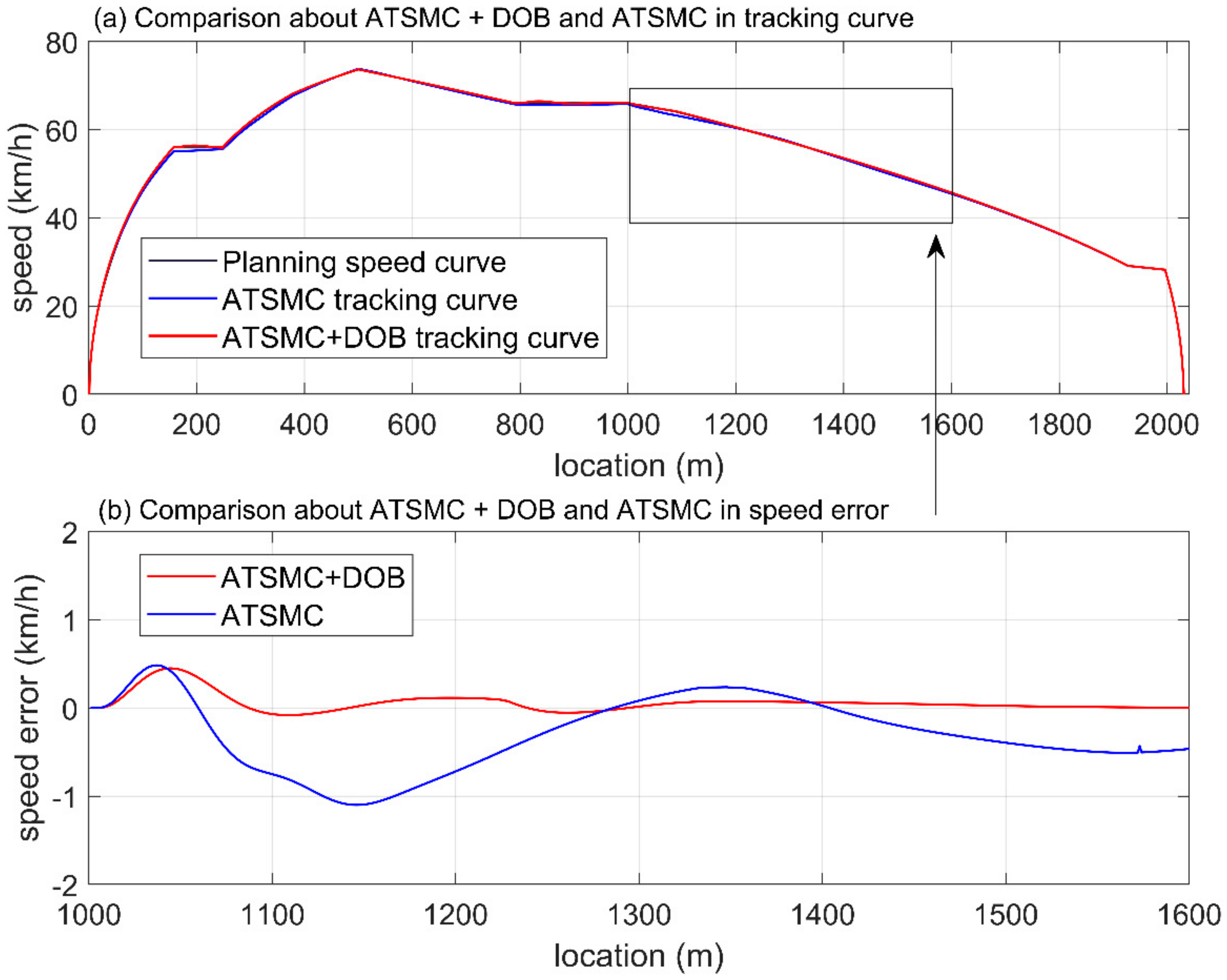
Compared with the ATSMC algorithm, as shown in the Figure 21, the disturbance observer significantly reduces the control error, especially when the train is running on a steep slope. Furthermore, compared with the PID algorithm, as shown in Figure 22, the ATSMC+DOB algorithm significantly reduces the speed error, which will greatly improve the comfort, punctuality, and parking accuracy of the train.

In addition, as the focus of our attention, as shown in Figure 23, due to the precise tracking of the ATSMC algorithm, although its energy consumption is slightly higher than that of the reference curve, it still much better than the PID algorithm, which has bad energy saving due to a large tracking error. In conclusion, the ATSMC+DOB algorithm performs good tracking accuracy.

The detail data are listed in

Table 9. Detailed data about the comparison.

Performance Indices	ATSMC+DOB	ATSMC	PID
Arrival time error (s)	1.2	1.4	6.7
Total consumption (kJ)	102,528	103,231	110,207
Average accelerated change rate (m/s3)	0.0371	0.0399	0.55
Average speed error (m/s)	0.05276	0.1933	0.8731
Stop error (m)	0.268	0.941	2.459

. The ATSMC+DOB algorithm performs better than the PID algorithm and the ATSMC algorithm in all indicators; PID algorithm is the worst, far worse than ATSMC+DOB algorithm and ATSMC algorithm. In terms of energy consumption, ATSMC+DOB is 7.58% lower than PID and 0.7% lower than ATSMC. Generally, the ATSMC+DOB algorithm perfectly meets the requirements of the metros for energy saving, punctuality, and comfortableness.

In addition, as we can see in Figure 21b, ATSMC+DOB has less speed errors than ATSMC, and ATSMC+DOB can converge faster. The detailed data in the table also prove this. The observer brings better anti-disturbance.

7. Conclusions

This paper carried out a series of researches on metro speed profile optimization and speed tracking control, and further designed corresponding algorithms and conducted simulation verification based on real data. The relevant conclusions are summarized as follows:

(1)

A multi-objective optimization model that considers energy consumption calculation and takes punctuality and comfortableness as penalty factors is established to optimize the train speed profile. This model takes the comfortableness of the metro and the punctuality into consideration when optimizing energy saving.

(2)

An optimization strategy that considers the metro EBI speed limit and the actual volume of the train (warning speed limit) is proposed. An improved ABC algorithm named RR-ABC algorithm is proposed for speed profile optimization. Compared with ordinary algorithms, the RR-ABC algorithm not only has good global search ability to avoid the local optimal solutions, but it also has excellent local search ability to improve the evolutionary efficiency.

(3)

A terminal sliding mode controller with disturbance observer (ATSMC+DOB) is designed by introducing parameter adaptation mechanism and disturbance observer. The controller has better robustness and anti-disturbance which brings minor speed tracking error and good energy saving.

(4)

The real data from Qingdao Metro Line 6 were used for the verification of the research. The simulation test results prove that the research on speed-profile optimization and speed-tracking control is effective.

The optimizations based on coast optimization and various speed limits proposed in the paper are targeted and only effective for a specific single interval, but for most metro lines, the conditions of each interval are different. Assuming that we design a different strategy for different intervals, it must not be a good way. Therefore, in future research, a more general optimization strategy is worthy of being studied.

References

1. Lu, S.; Hillmansen, S.; Ho, T.K.; Roberts, C. Single-train trajectory optimization. IEEE Trans. Intell. Transp. Syst. 2013, 14, 743–750. [Google Scholar] [CrossRef]
2. Li, Z.; Tang, T.; Gao, C. Long short-term memory neural network applied to train dynamic model and speed prediction. Algorithms 2019, 12, 173. [Google Scholar] [CrossRef] [Green Version]
3. Su, S.; Li, X.; Tang, T.; Gao, Z.Y. A Subway Train Timetable Optimization Approach Based on Energy-Efficient Operation Strategy. IEEE Trans. Intell. Transp. Syst. 2013, 14, 883–893. [Google Scholar] [CrossRef]
4. Wang, B.; Yang, J.; Jiao, H.N.; Zhu, K.; Chen, Y.Q. Design of auto disturbance rejection controller for train traction control system based on artificial bee colony algorithm. Measurement 2020, 160, 9. [Google Scholar] [CrossRef]
5. Guo, X.; Wang, J.L.; Liao, F.; Teo, R. Distributed adaptive sliding mode control strategy for vehicle-following systems with nonlinear acceleration uncertainties. IEEE Trans. Veh. Technol. 2017, 66, 981–991. [Google Scholar] [CrossRef]
6. Tan, C.K.; Wang, J.; Paw, Y.C.; Ng, T.Y. Tracking of a moving ground target by a quadrotor using a backstepping approach based on a full state cascaded dynamic. Appl. Soft Comput. 2016, 47, 47–62. [Google Scholar] [CrossRef]
7. Bidikli, B. An observer-based adaptive control design for the maglev system. Trans. Inst. Meas. Control 2020, 42, 2771–2786. [Google Scholar] [CrossRef]
8. Song, Y.D.; Song, Q.; Cai, W.C. Fault-tolerant adaptive control of high-speed trains under traction/braking failures: A virtual parameter-based approach. IEEE Trans. Intell. Transp. Syst. 2014, 15, 737–748. [Google Scholar] [CrossRef]
9. Wang, Y.; Song, Y.; Gao, H.; Lewis, F.L. Distributed fault-tolerant control of virtually and physically interconnected systems with application to high-speed trains under traction/braking failures. IEEE Trans. Intell. Transp. Syst. 2016, 17, 535–545. [Google Scholar] [CrossRef]
10. Lin, X.; Dong, H.; Yao, X.; Bai, W. Neural adaptive fault-tolerant control for high-speed trains with input saturation and unknown disturbance. Neurocomputing 2017, 260, 32–42. [Google Scholar] [CrossRef]
11. Chen, Z.; Huang, F.H.; Chen, W.J.; Zhang, J.H.; Sun, W.C.; Chen, J.W.; Gu, J.; Zhu, S.Q. RBFNN-based adaptive sliding mode control design for delayed nonlinear multilateral telerobotic system with cooperative manipulation. IEEE Trans. Ind. Inform. 2020, 16, 1236–1247. [Google Scholar] [CrossRef]
12. Qiao, L.; Zhang, W.D. Trajectory tracking control of AUVs via adaptive fast nonsingular integral terminal sliding mode control. IEEE Trans. Ind. Inform. 2020, 16, 1248–1258. [Google Scholar] [CrossRef]
13. Liu, X.D.; Yu, H.S.; Yu, J.P.; Zhao, L. Combined speed and current terminal sliding mode control with nonlinear disturbance observer for PMSM Drive. IEEE Access 2018, 6, 29594–29601. [Google Scholar] [CrossRef]
14. Cao, W.J.; Xu, J.X. Nonlinear integral-type sliding surface for both matched and unmatched uncertain systems. IEEE Trans. Automat. Contr. 2004, 49, 1355–1360. [Google Scholar] [CrossRef]
15. Van, M.; Mavrovouniotis, M.; Ge, S.S. An adaptive backstepping nonsingular fast terminal sliding mode control for robust fault tolerant control of robot manipulators. IEEE Trans. Syst. Man Cybern. Syst. 2019, 49, 1448–1458. [Google Scholar] [CrossRef] [Green Version]
16. Yang, X.; Chen, A.; Ning, B.; Tang, T. A stochastic model for the integrated optimization on metro timetable and speed profile with uncertain train mass. Transp. Res. Part B Methodol. 2016, 91, 424–445. [Google Scholar] [CrossRef]
17. Howlett, P. The optimal control of a train. Ann. Oper. Res. 2000, 98, 65–87. [Google Scholar] [CrossRef]
18. Howlett, P. An optimal strategy for the control of a train. Anziam J. 1990, 31, 454–471. [Google Scholar] [CrossRef] [Green Version]
19. Koopialipoor, M.; Armaghani, D.J.; Haghighi, M.; Ghaleini, E.N. A neuro-genetic predictive model to approximate overbreak induced by drilling and blasting operation in tunnels. Bull. Eng. Geol. Environ. 2019, 78, 981–990. [Google Scholar] [CrossRef]
20. Su, S.; Tang, T.; Li, X. Driving strategy optimization for trains in subway systems. Proc. Inst. Mech. Eng. Part F 2018, 232, 369–383. [Google Scholar] [CrossRef]
21. Chuang, H.J.; Chen, C.S.; Lin, C.H.; Hsieh, C.H.; Ho, C.Y. Design of optimal coasting speed for MRT systems using ANN models. IEEE Trans. Ind. Appl. 2009, 45, 2090–2097. [Google Scholar] [CrossRef]
22. Khmelnitsky, E. On an optimal control problem of train operation. IEEE Trans. Autom. Control 2000, 45, 1257–1266. [Google Scholar] [CrossRef]
23. Sheu, J.W.; Lin, W.S. Energy-saving automatic train regulation using dual heuristic programming. IEEE Trans. Veh. Technol. 2012, 61, 1503–1514. [Google Scholar] [CrossRef]
24. Song, Y.; Song, W. A novel dual speed-curve optimization-based approach for energy-saving operation of high-speed trains. IEEE Trans. Intell. Transp. Syst. 2016, 17, 1–12. [Google Scholar] [CrossRef]
25. Cheng, R.J.; Song, Y.D.; Chen, D.W.; Ma, X.P. Intelligent positioning approach for high speed trains based on ant colony optimization and machine learning algorithms. IEEE Trans. Intell. Transp. Syst. 2019, 20, 3737–3746. [Google Scholar] [CrossRef]
26. Karaboga, D.; Basturk, B. A powerful and efficient algorithm for numerical function optimization: Artificial Bee Colony (ABC) algorithm. J. Glob. Optim. 2007, 39, 459–471. [Google Scholar] [CrossRef]
27. Youneng, H.; Chen, Y.; Shaofeng, G. Energy optimization for train operation based on an improved ant colony optimization methodology. Energies 2016, 9, 626. [Google Scholar]
28. Rocha, A.; Araújo, A.; Carvalho, A.; Sepulveda, J. A new approach for real time train energy efficiency optimization. Energies 2018, 11, 2660. [Google Scholar] [CrossRef] [Green Version]
29. Tan, Z.; Lu, S.; Bao, K.; Zhang, S.; Wu, C.; Yang, J.; Xue, F. Adaptive partial train speed trajectory optimization. Energies 2018, 11, 3302. [Google Scholar] [CrossRef] [Green Version]
30. Farooqi, H.; Incremona, G.P.; Colaneri, P. Railway collaborative eco drive via dissension-based switching nonlinear model predictive control. Eur. J. Control 2019, 50, 153–160. [Google Scholar] [CrossRef] [Green Version]
31. Yan, X.H.; Cai, B.G.; Ning, B.; Wei, S.G. Online distributed cooperative model predictive control of energy-saving trajectory planning for multiple high-speed train movements. Transp. Res. Part C 2016, 69, 60–78. [Google Scholar] [CrossRef]
32. Chen, M.; Xiao, Z.; Sun, P.; Wang, Q.; Jin, B.; Feng, X. Energy efficient driving strategies for multi-train by optimization and update speed profiles considering transmission losses of regenerative energy. Energies 2019, 12, 3573. [Google Scholar] [CrossRef] [Green Version]
33. Cao, Y.; Wang, Z.C.; Liu, F.; Li, P.; Xie, G. Bio-inspired speed curve optimization and sliding mode tracking control for subway trains. IEEE Trans. Veh. Technol. 2019, 68, 6331–6342. [Google Scholar] [CrossRef]
34. Shang, F.; Zhan, J.; Chen, Y. An online energy-saving driving strategy for metro train operation based on the model predictive control of switched-mode dynamical systems. Energies 2020, 13, 4933. [Google Scholar] [CrossRef]
35. Huang, Y.N.; Bai, S.; Meng, X.H.; Yu, H.Z.; Wang, M.Z. Research on the driving strategy of heavy-haul train based on improved genetic algorithm. Adv. Mech. Eng. 2018, 10, 16. [Google Scholar] [CrossRef] [Green Version]
36. Liu, D.; Zhu, S.Q.; Xu, Y.X.; Liu, K. Train operation optimization with adaptive differential evolution algorithm based on decomposition. IEEJ Trans. Electr. Electron. Eng. 2019, 14, 1772–1779. [Google Scholar] [CrossRef]
37. Li, X.; Lo, H.K. An energy-efficient scheduling and speed control approach for metro rail operations. Transp. Res. Part B-Methodol. 2014, 64, 73–89. [Google Scholar] [CrossRef]
38. ISO. ISO 2631-5: 2018. Mechanical Vibration and Shock—Evaluation of Human Exposure to Whole-Body Vibration of International Standard; ISO: Geneva, Switzerland, 2018. [Google Scholar]
39. Banharnsakun, A.; Achalakul, T.; Sirinaovakul, B. The best-so-far selection in artificial bee colony algorithm. Appl. Soft. Comput. 2011, 11, 2888–2901. [Google Scholar] [CrossRef]
40. Kiran, M.S.; Hakli, H.; Gunduz, M.; Uguz, H. Artificial bee colony algorithm with variable search strategy for continuous optimization. Inf. Sci. 2015, 300, 140–157. [Google Scholar] [CrossRef]
41. Utkin, V.; Guldner, J.; Shi, J. Sliding Mode Control in Electro-Mechanical Systems, 2nd ed.; CRC Press: New York, NY, USA, 2009; pp. 159–203. [Google Scholar]
42. Ferrara, A.; Incremona, G.P.; Cucuzzella, M. Advanced and Optimization Based Sliding Mode Control: Theory and Applications; Society for Industrial and Applied Mathematics (SIAM): Philadelphia, PA, USA, 2019. [Google Scholar]
43. Sariyildiz, E.; Oboe, R.; Ohnishi, K. Disturbance observer-based robust control and its applications: 35th anniversary overview. IEEE Trans. Ind. Electron. 2020, 67, 2042–2053. [Google Scholar] [CrossRef] [Green Version]
44. Huang, J.; Zhang, M.S.; Ri, S.; Xiong, C.H.; Li, Z.J.; Kang, Y. High-order disturbance-observer-based sliding mode control for mobile wheeled inverted pendulum systems. IEEE Trans. Ind. Electron. 2020, 67, 2030–2041. [Google Scholar] [CrossRef]
Figure 1. Force analysis of single particle model.
Energies 13 06093 g001
Figure 2. External characteristic curve of traction force and braking force.
Energies 13 06093 g002
Figure 3. Train multi-interval operation planning.
Energies 13 06093 g003
Figure 4. Subinterval division.
Energies 13 06093 g004
Figure 5. Punctuality penalty function.
Energies 13 06093 g005
Figure 6. Comfortableness penalty function.
Energies 13 06093 g006
Figure 7. Three stages in emergency braking intervention (EBI) protection.
Energies 13 06093 g007
Figure 8. Safety speed limit.
Energies 13 06093 g008
Figure 9. Speed-limit curve.
Energies 13 06093 g009
Figure 10. Coast strategy.
Energies 13 06093 g010
Figure 11. Comparison of classic method and reinforcement method.
Energies 13 06093 g011
Figure 12. Controller model.
Energies 13 06093 g012
Figure 13. Disturbance observer structure.
Energies 13 06093 g013
Figure 14. Comparison of evolutionary performance: (a) Comparison about RR-ABC and ABC; (b) Comparison about RR-ABC and GA.
Energies 13 06093 g014
Figure 15. Optimal speed profile: (a) The optimal speed profile made by optimization; (b) Cumulative energy consumption growth curve.
Energies 13 06093 g015
Figure 16. Optimal speed profile. (a) The optimal speed profile made by optimization; (b) Cumulative energy consumption growth curve.
Energies 13 06093 g016
Figure 17. Optimal speed profile. (a) The optimal speed profile made by optimization; (b) Cumulative energy consumption growth curve.
Energies 13 06093 g017
Figure 18. Comparison of different driving modes: (a) Comparison about coast mode and cruise mode in speed profile; (b) Comparison about coast mode and cruise mode in cumulative energy consumption curve.
Energies 13 06093 g018
Figure 19. Experiment 1 and Experiment 2.
Energies 13 06093 g022
Figure 20. Experiment 3 and Experiment 4.
Energies 13 06093 g023
Figure 21. Comparison of adaptive terminal sliding mode controller (ATSMC) and ATSMC+disturbance observer (DOB): (a) Comparison in speed curve; (b) Comparison in speed error.
Energies 13 06093 g019
Figure 22. Comparison of PID and ATSMC+DOB: (a) Comparison in tracking curve; (b) Comparison in speed error.
Energies 13 06093 g020
Figure 23. Comparison of energy consumption of different controllers.
Energies 13 06093 g021