Application of Equilibrium Optimizer Algorithm for Optimal Power Flow with High Penetration of Renewable Energy
Abstract
1. Introduction
1.1. Background
1.2. Literature Review
1.3. Contribution and Paper Organization
2. Problem Formulation of OPF
2.1. General Structure of OPF
2.2. Objective Functions of OPF
- Case 1: real power loss minimization
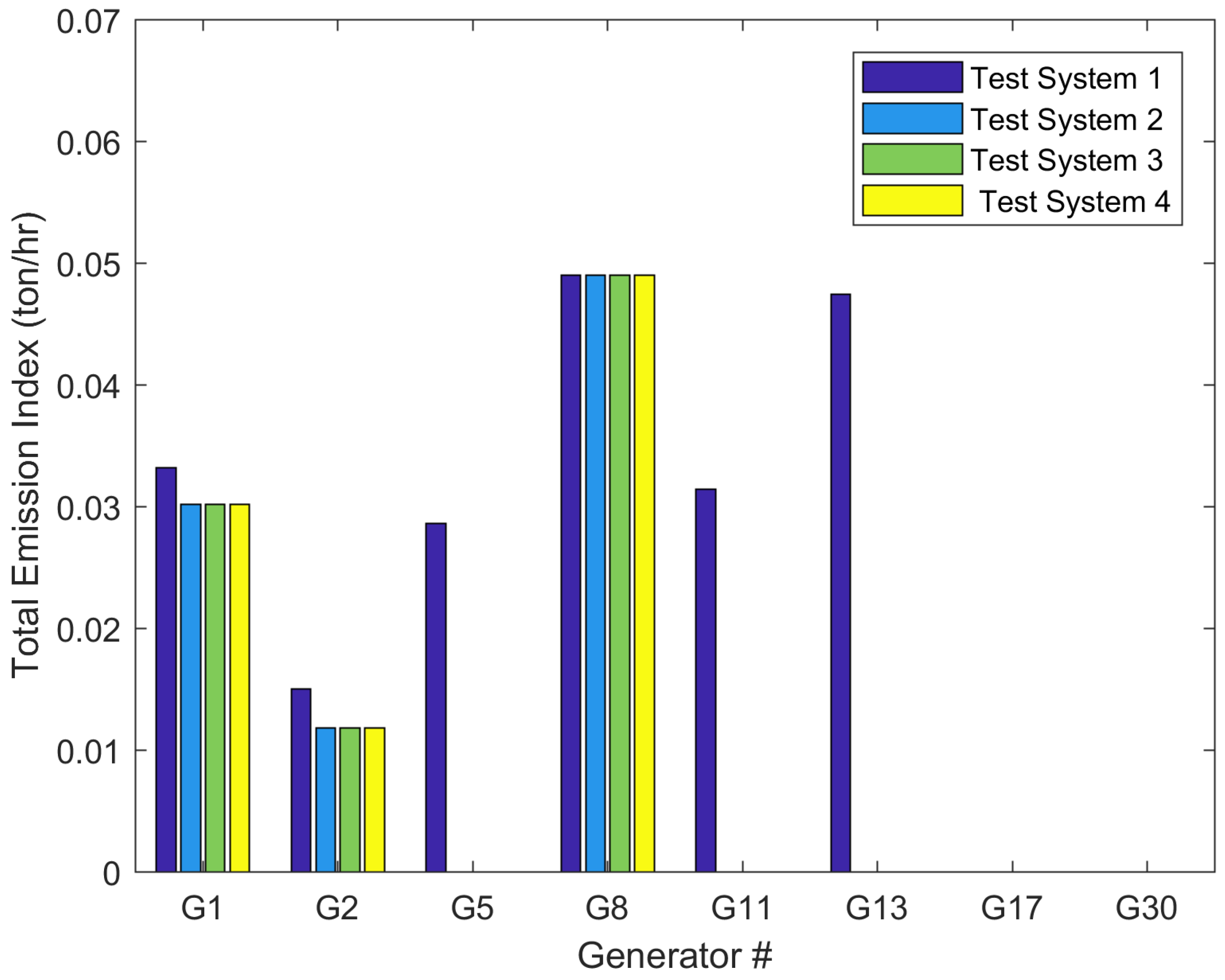
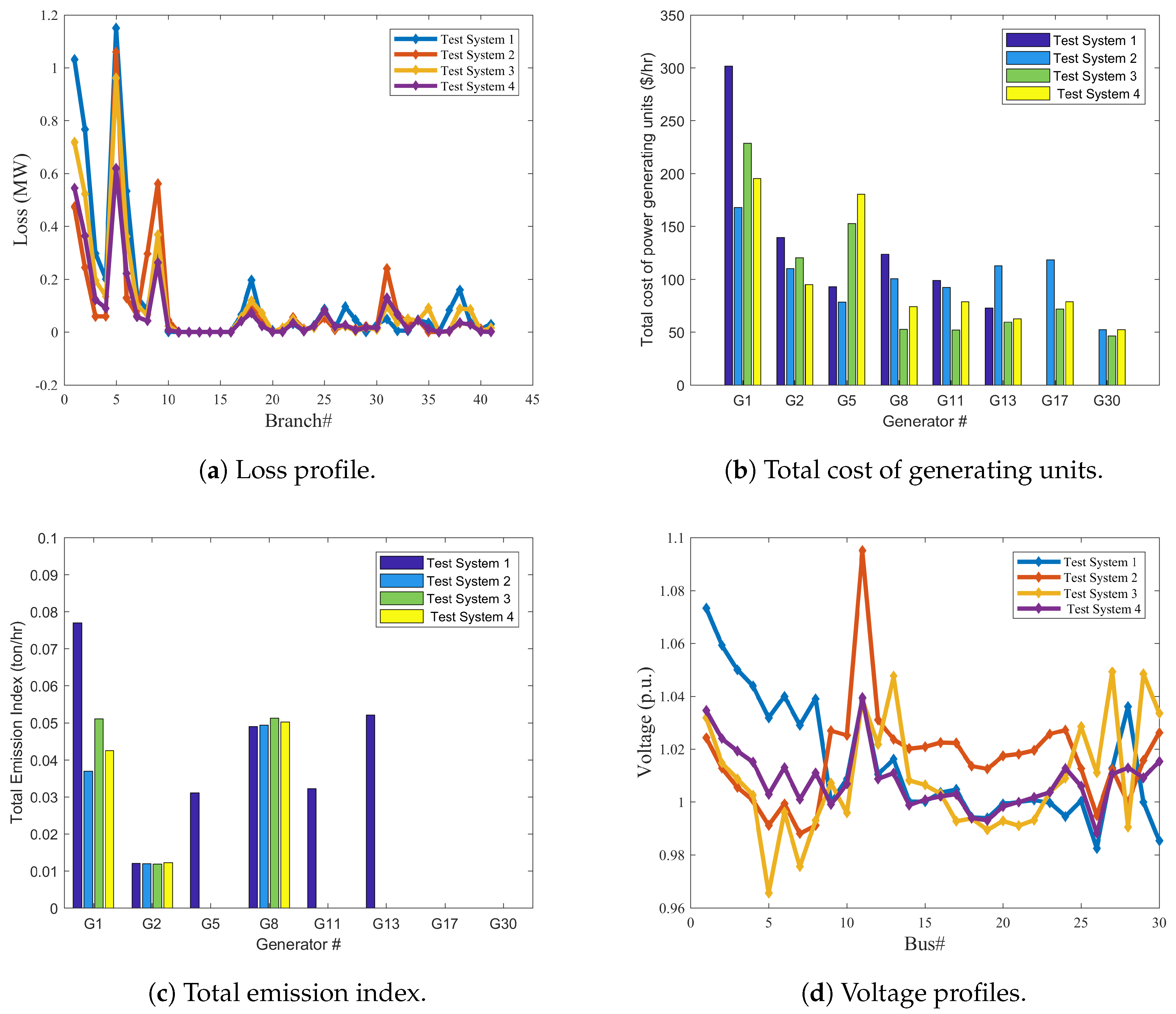
- Case 2: emission index minimizationIn the present case, the target is to reduce the harmful gases emission from the thermal generation units, and the coefficients of the gas emission of the thermal power generators are given in Table 1. Emission in tons per hour (t/h) can be described by [14,35]:where , , , and are the emission coefficients and G1, G2, G3, G4, G5, and G6 represent thermal power generators at buses 1, 2, 5, 8, 11, and 13, respectively, as given in Table 1.
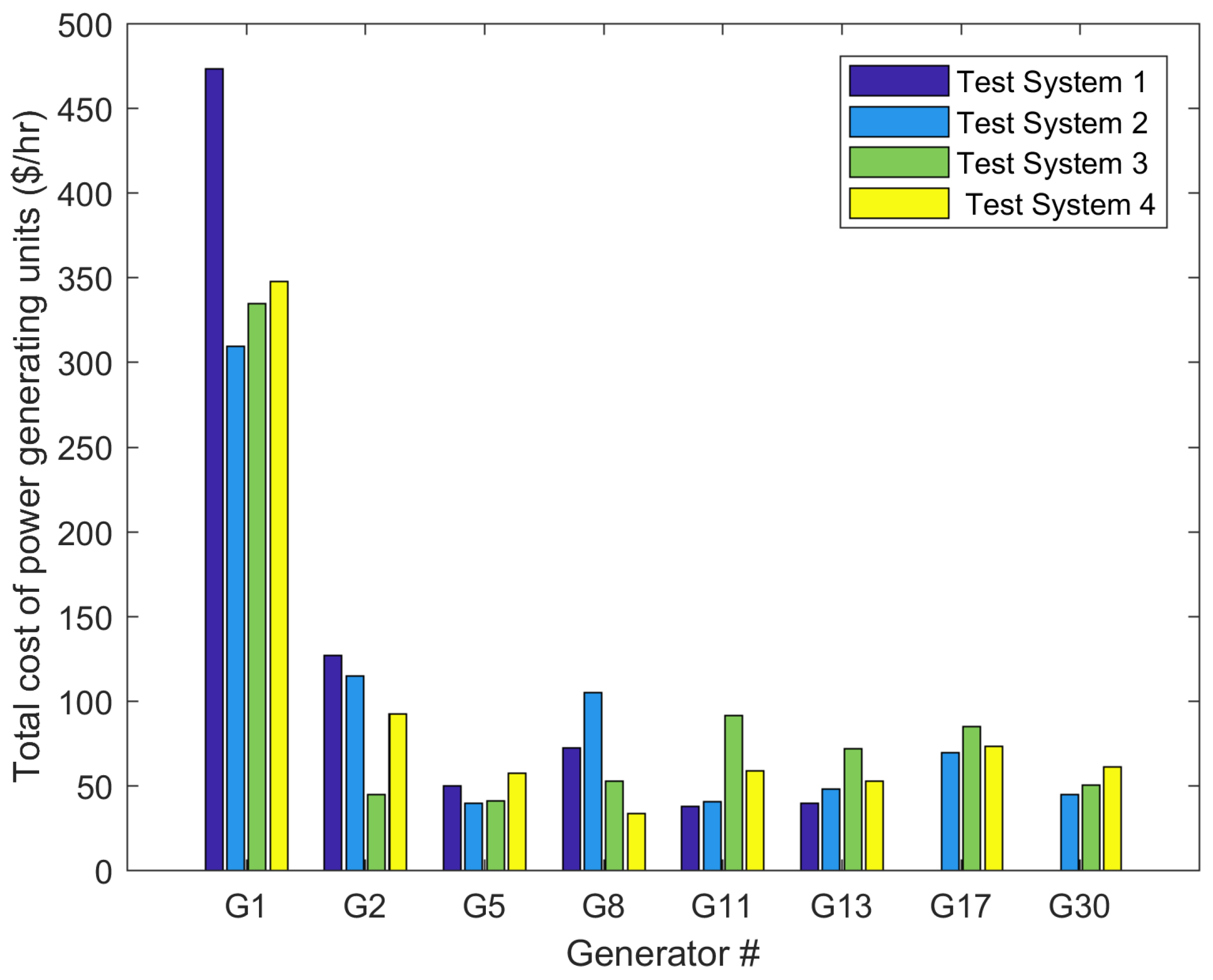
- Case 3: Basic fuel cost minimization
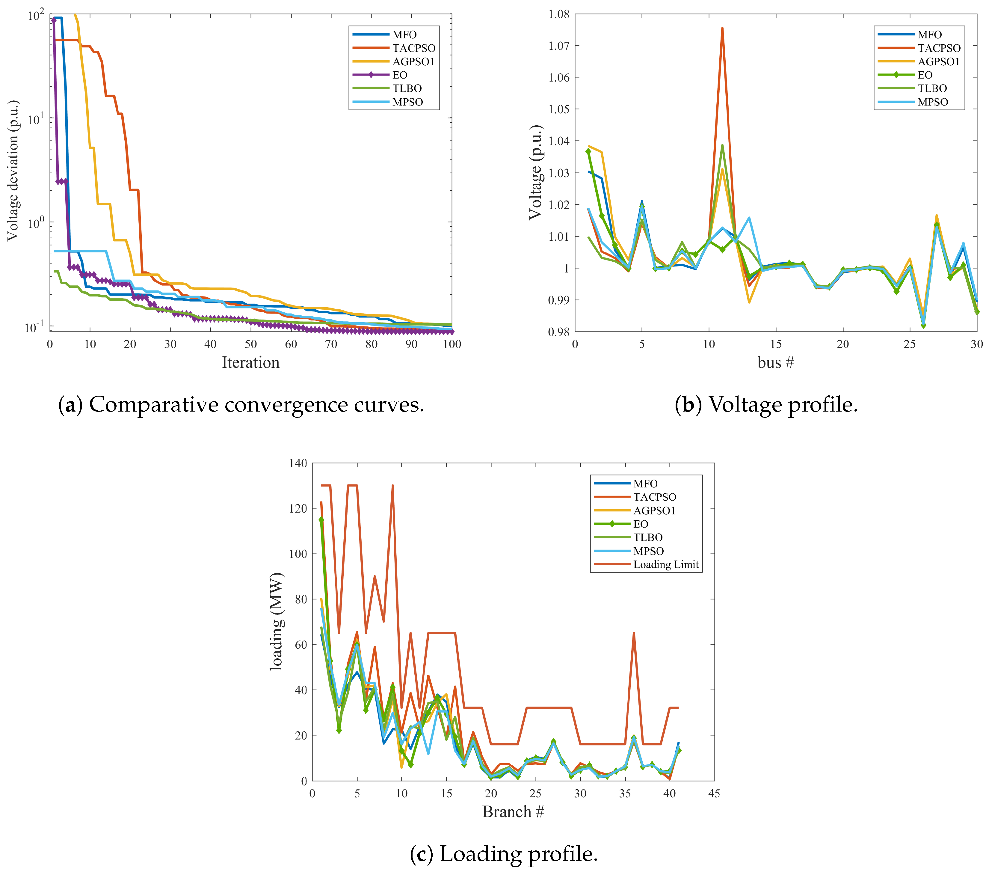
- Case 4: Voltage deviation minimization
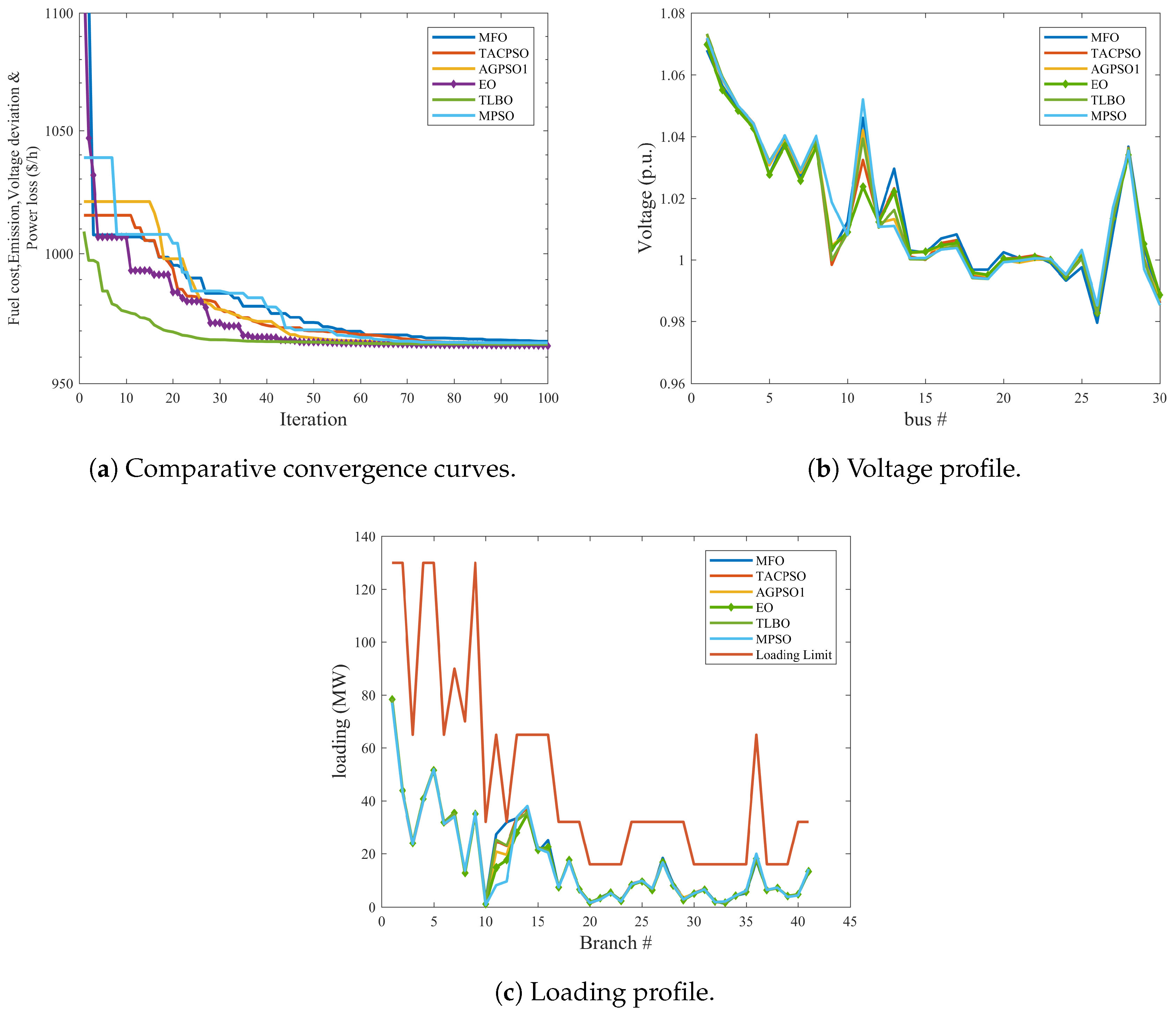
- Case 5: Minimization of basic the fuel cost, emission index, voltage deviation and the real power losses.
2.3. Constraints
- Equality constraintsThe equality constraints of OPF are usually represented by the load flow equations:where , , , and are the active and reactive load demand, the number of buses and the angle difference between bus i and k, respectively. and are the transfer and susceptance conductance.
- Inequality constraintsIt can be defined by operating limits on the equipment of the power system, transmission loading and voltage of load buses.
- (a)
- Constraints of thermal and renewable energy generating units
- (b)
- Constraints of the transformer tap setting
- (c)
- constraints of the shunt compensator
- (d)
- Constraints of the voltages at load buses
- (e)
- Constraints of the transmission line loading
2.4. Constraint Handling
3. Mathematical Models of the Wind and Solar Power Generating Units
3.1. Wind Power Units
3.1.1. Uncertain and Power Model of Wind Turbines
3.1.2. Calculation of Direct, Underestimation and Overestimation Cost of Wind Power
3.2. Solar Power Units
3.2.1. Uncertain and Power Model of Solar PV Plants
3.2.2. Calculation of Direct, Underestimation, and Overestimation Cost of Solar PV Power
4. Proposed EO
4.1. Inspiration and Mathematical Model
4.2. The Interaction between Each Term and the Search Pattern and the Definition of the EO’s Terms
4.2.1. Initialization and Function Evaluation
4.2.2. Equilibrium Pool and Candidates ()
4.2.3. Exponential Term (F)
4.2.4. The Generation Rate (G)
4.2.5. Particle’s Memory Saving
4.3. Implementation of EO to Solve the OPF Problem
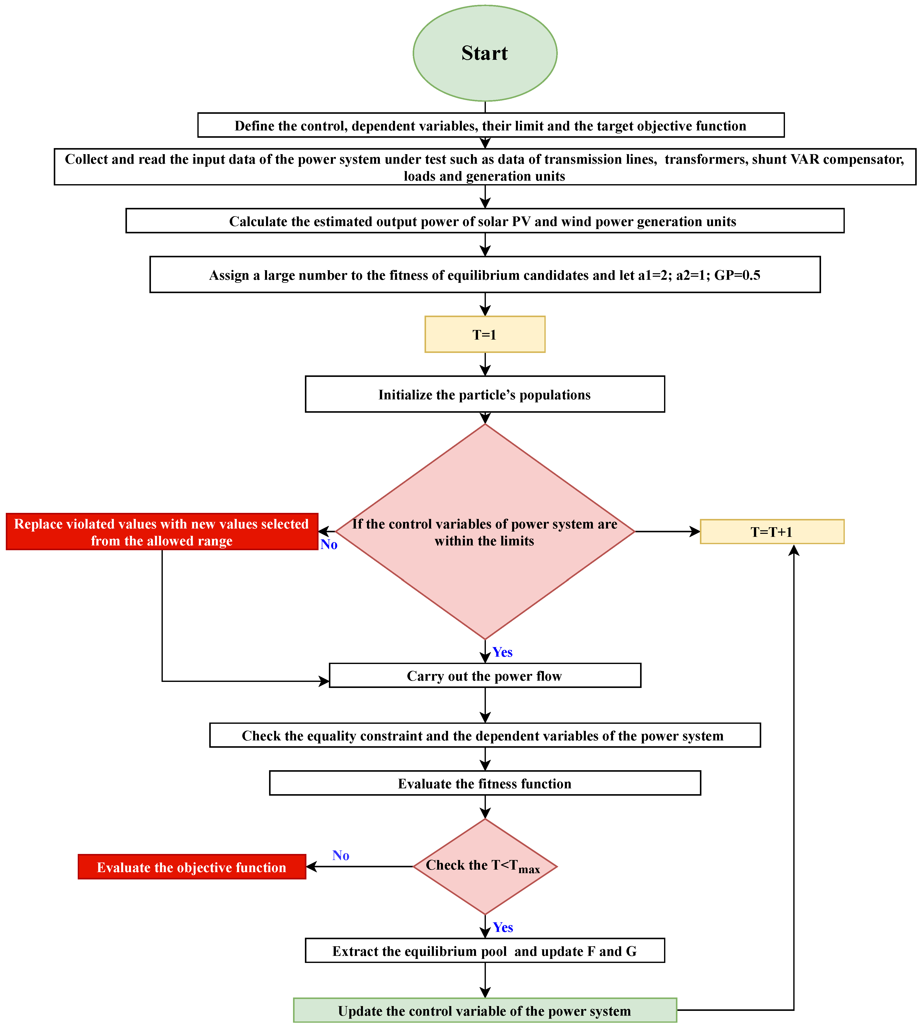
- Define the control and dependent variables and their limits, as well as the target objective function defined in Section 2.2 [34].
- Collect and read the input data of the power system under test, such as data of transmission lines, transformers, shunt VAR compensator, loads and generation units.
- Initialize the particle’s populations [34].
- Assign a large number to the fitness of equilibrium candidates and let a1 = 2; a2 = 1; GP = 0.5 [34].
- Do the main while loop as the following [34]:
- (a)
- While (current iteration (Iter) <maximum number of iteration (Max-iter))
- (b)
- For i=1: particles’ number (n)
- (c)
- Find the fitness value of the particle
- If fitness () <fitness () thenSubstitute () with () and fitness ()with fitness ()
- Else if fitness () >fitness () & fitness () <fitness () thenSubstitute () with () and fitness ()with fitness ()
- Else if fitness () >fitness () & fitness () >fitness () & fitness () <fitness () thenSubstitute () with () and fitness ()with fitness ()
- Else if fitness () >fitness () & fitness () >fitness () & fitness () >fitness () & fitness () <fitness () thenSubstitute () with () and fitness () with fitness ()
- (d)
- End (if)
- (e)
- End (for)
- Find the according to Equation (37).
- In case of the current iteration >1, accomplish memory saving [34].
- Assign t according to Equation (39).
- Do the second for loop as following:For i=1: particles’ number
- (a)
- Select one candidate from the equilibrium pool randomly.
- (b)
- Create the two random vector ( and r).
- (c)
- (d)
- Update the concentration C according to Equation (45)
End the second for loop. - Increase the current iteration by one.
- End the main while loop.
- Extract and analyse of the results.
5. Test Systems and Control Parameters of Optimization Methods
5.1. Description of the Test Power Systems
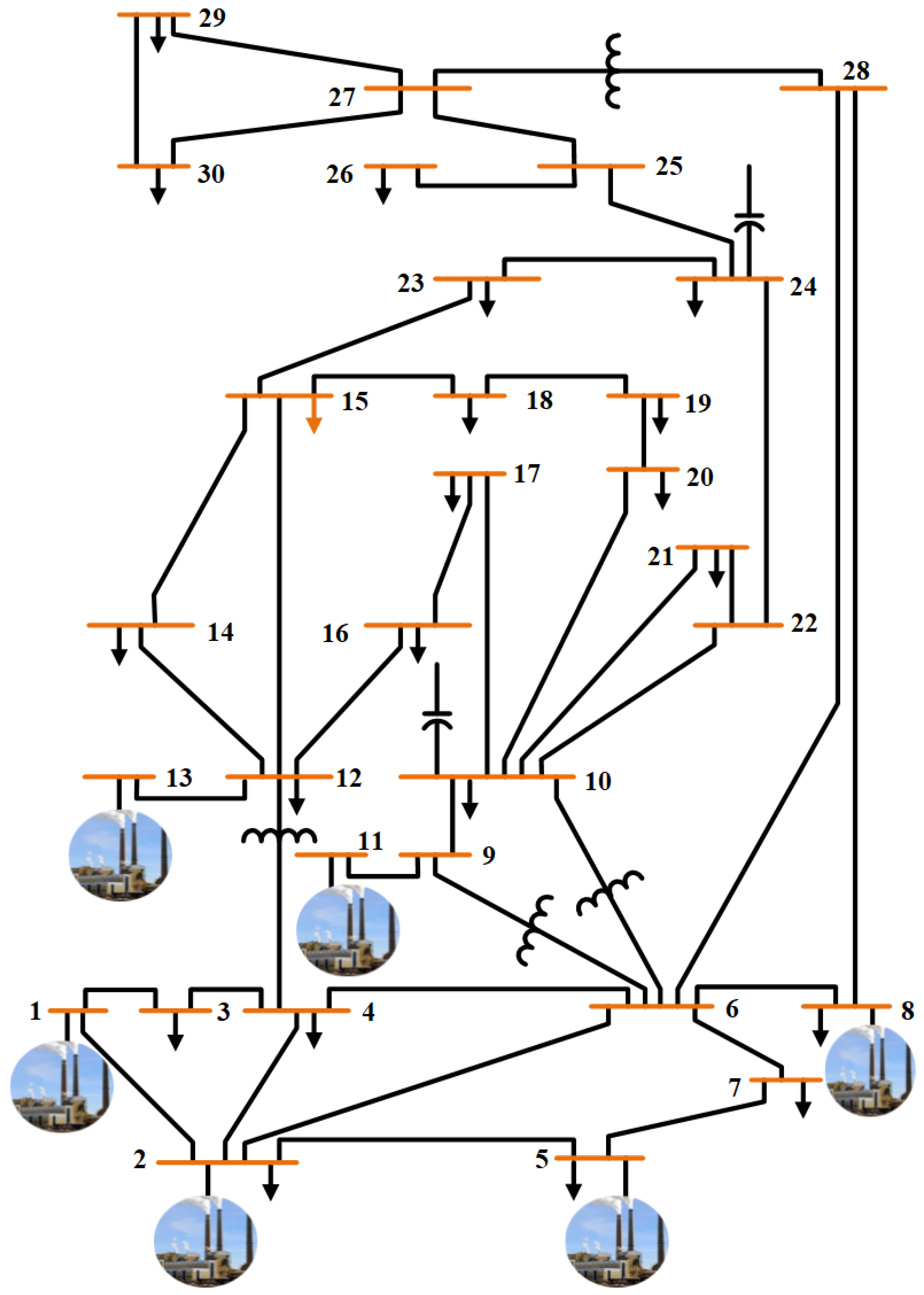
- Test system 1: IEEE 30-bus systemThe IEEE 30-bus system consists of six thermal power generators, as presented in Figure 2. The data about transmission lines, tap changing transformers, AVR compensators, limitations on generators and load voltages, active and reactive power demand are given in [42,43,44]. The general specifications of this system are described in Table 3.
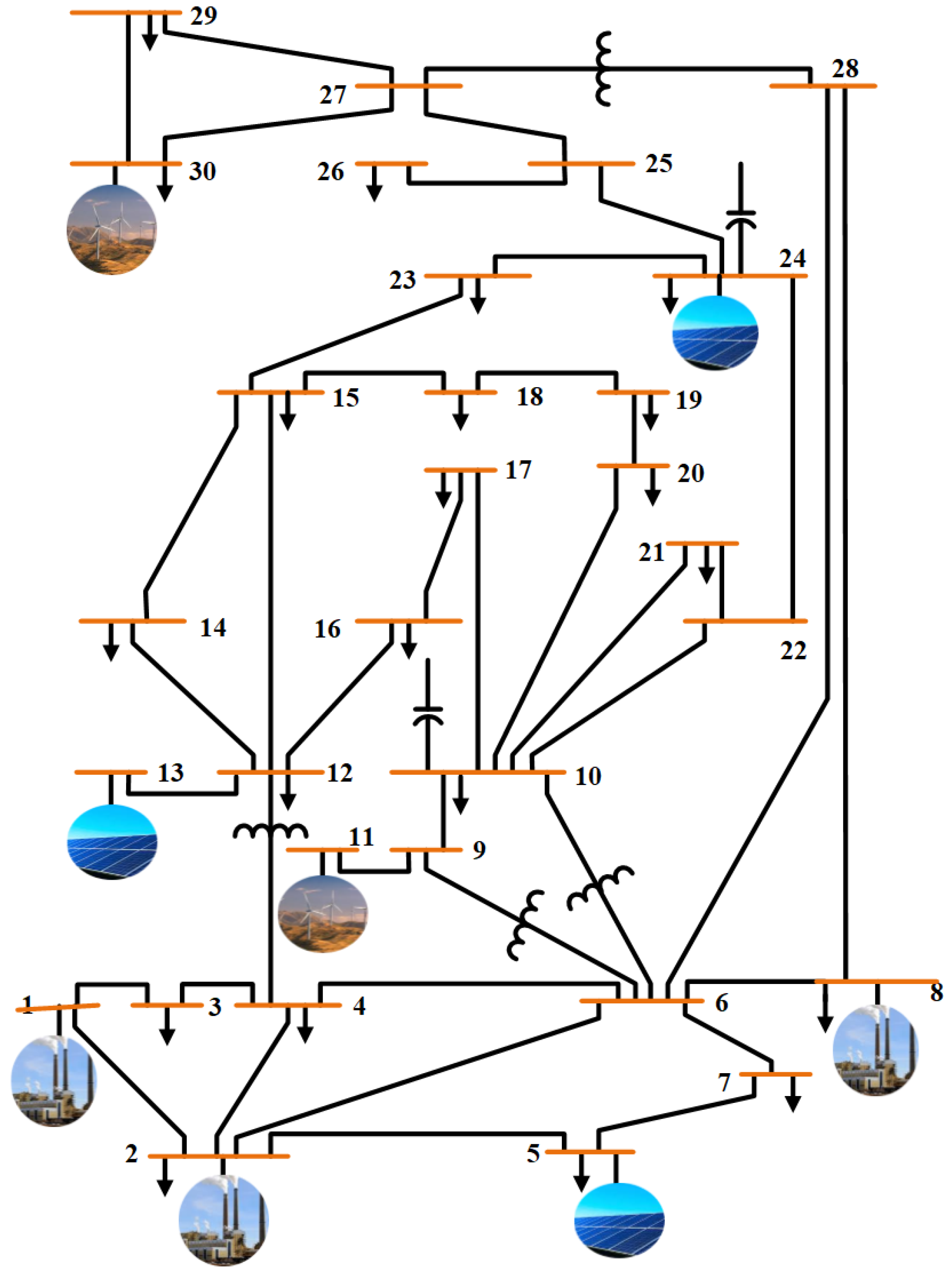
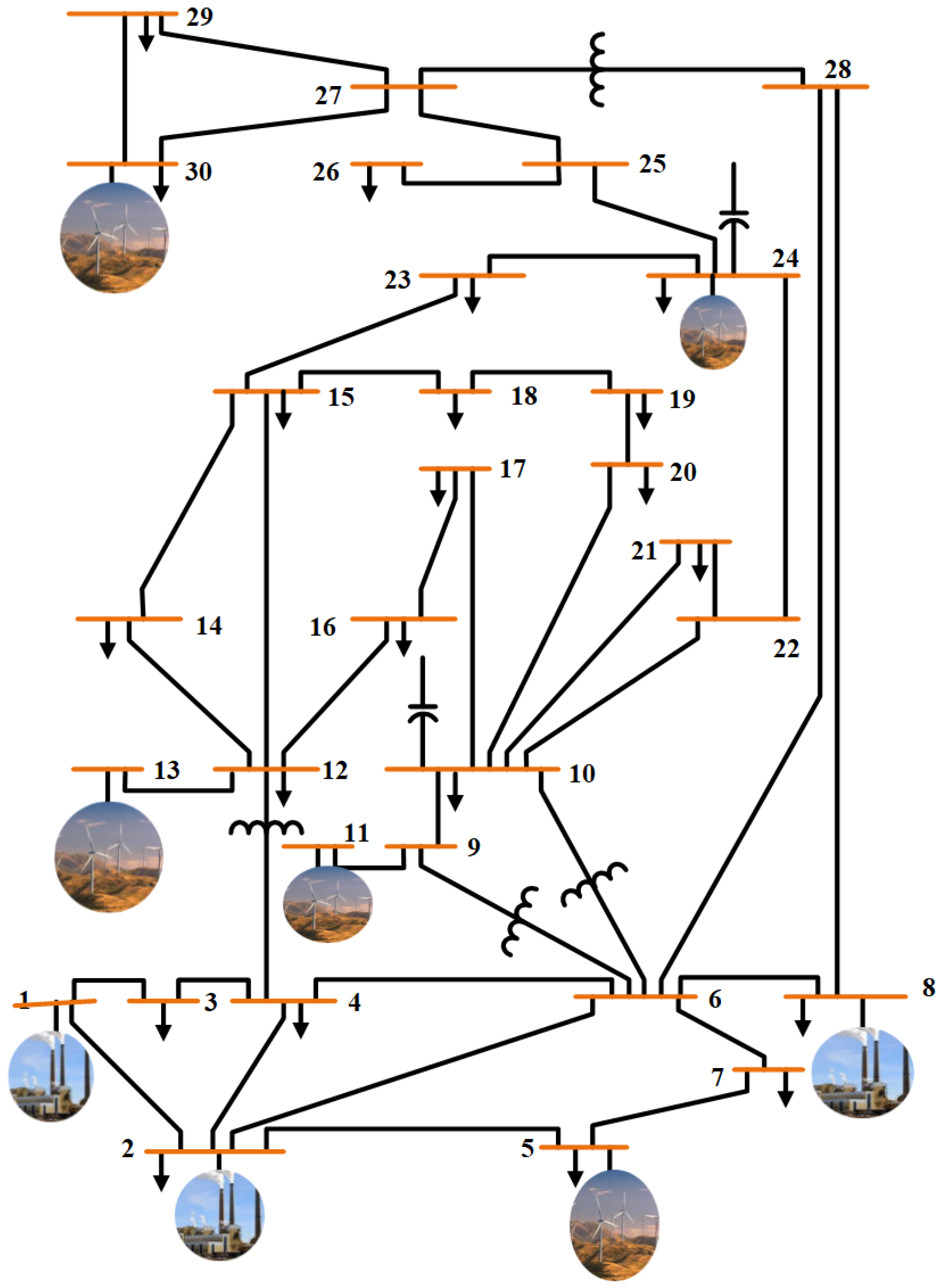
- Test system 2: Hybrid wind and solar PV integrated IEEE 30-bus systemThis modified test power system is simulated to show its behavior in the presence of both wind and solar PV power generating units, as depicted in Figure 3. The IEEE 30-bus system has been modified by replacing the thermal power generating units at buses 5, 11, and 13 with wind generator at bus 11 and solar PV at buses 5 and 13. In addition, the new solar PV and wind power generators are constructed at bus 24, and 30, respectively. The objective functions defined in Section 2.2 are modified by adding the output power of solar PV plants () and the output power of wind plants () given in Section 3. Case 3 and case 5 described in Section 2.2 are modified by adding the total cost of solar PV plants () and the total cost of wind plants () defined in Section 3. The specification of this hybrid power system is given in Table 3. The data of wind and solar PV plants are described in Table 4 and Table 5, respectively.
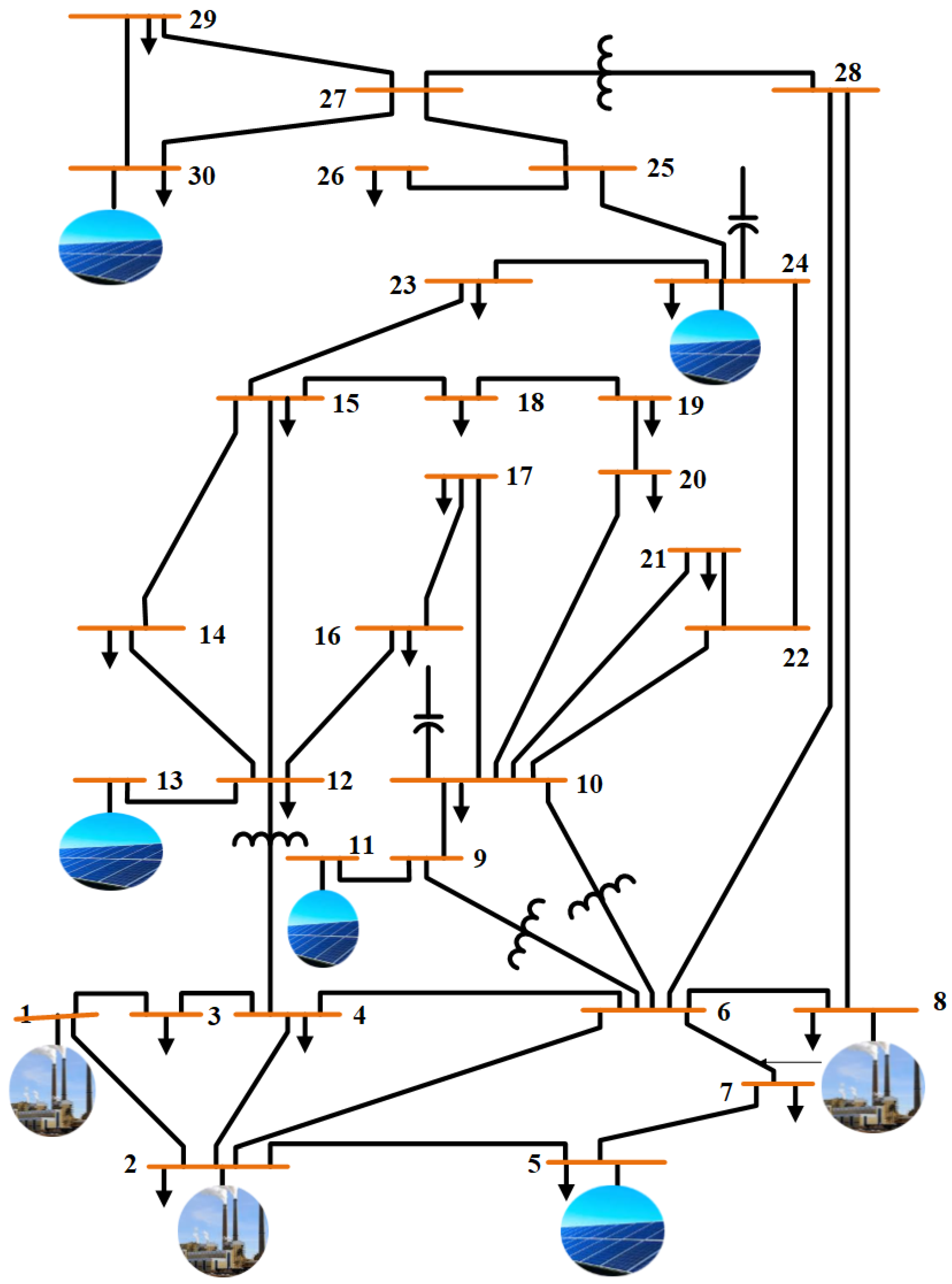
- Test system 3: Solar PV integrated IEEE 30-bus systemThis system is modified by locating solar PV generators at buses 5, 11, and 13 instead of the thermal power generators. Furthermore, two new solar power generation units are installed at buses 24, and 30, as shown in Figure 4. The objective funtions defined in Section 2.2 are modified by adding the output power of solar PV plants () given in Section 3. Case 3 and case 5 described in Section 2.2 are modified by adding the total cost of solar PV plants () defined in Section 3. The general data of this system and solar PV plants are presented in Table 3 and Table 6, respectively.
- Test system 4: wind integrated IEEE 30-bus systemIn this system, the IEEE 30-bus system is modified by replacing the thermal power generating units at buses 5, 11, and 13 with wind power generators. Moreover, two new wind generators have been added at buses 24, and 30, as seen in Figure 5. The objective functions defined in Section 2.2 is modified by adding the output power of wind plants () given in Section 3. Case 3 and case 5 described in Section 2.2 are modified by adding the total cost of wind plants () defined in Section 3. The general specifications of this system and the data of wind power plants are given in Table 3 and Table 7, respectively.
5.2. Control Parameters of Optimization Methods
6. Results and Discussion
6.1. Discussion and Analysis of the Objective Functions of OPF
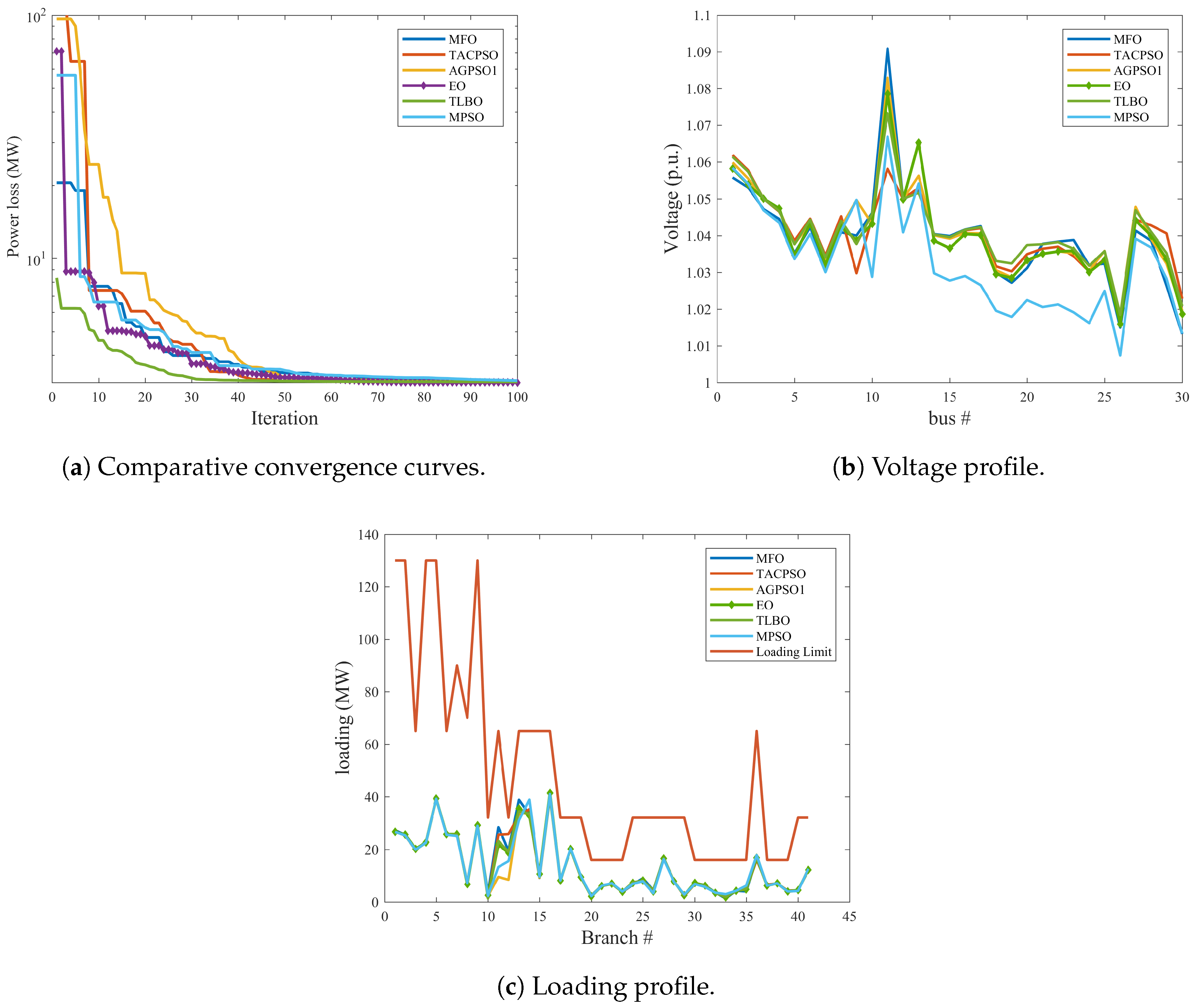
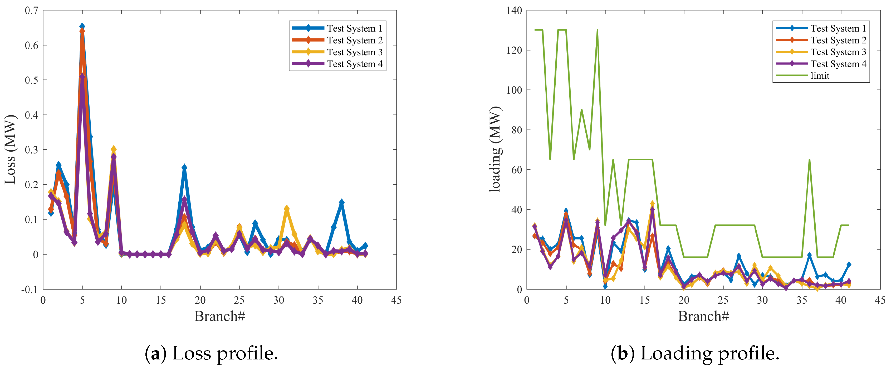
6.1.1. Minimization of Real Power Loss
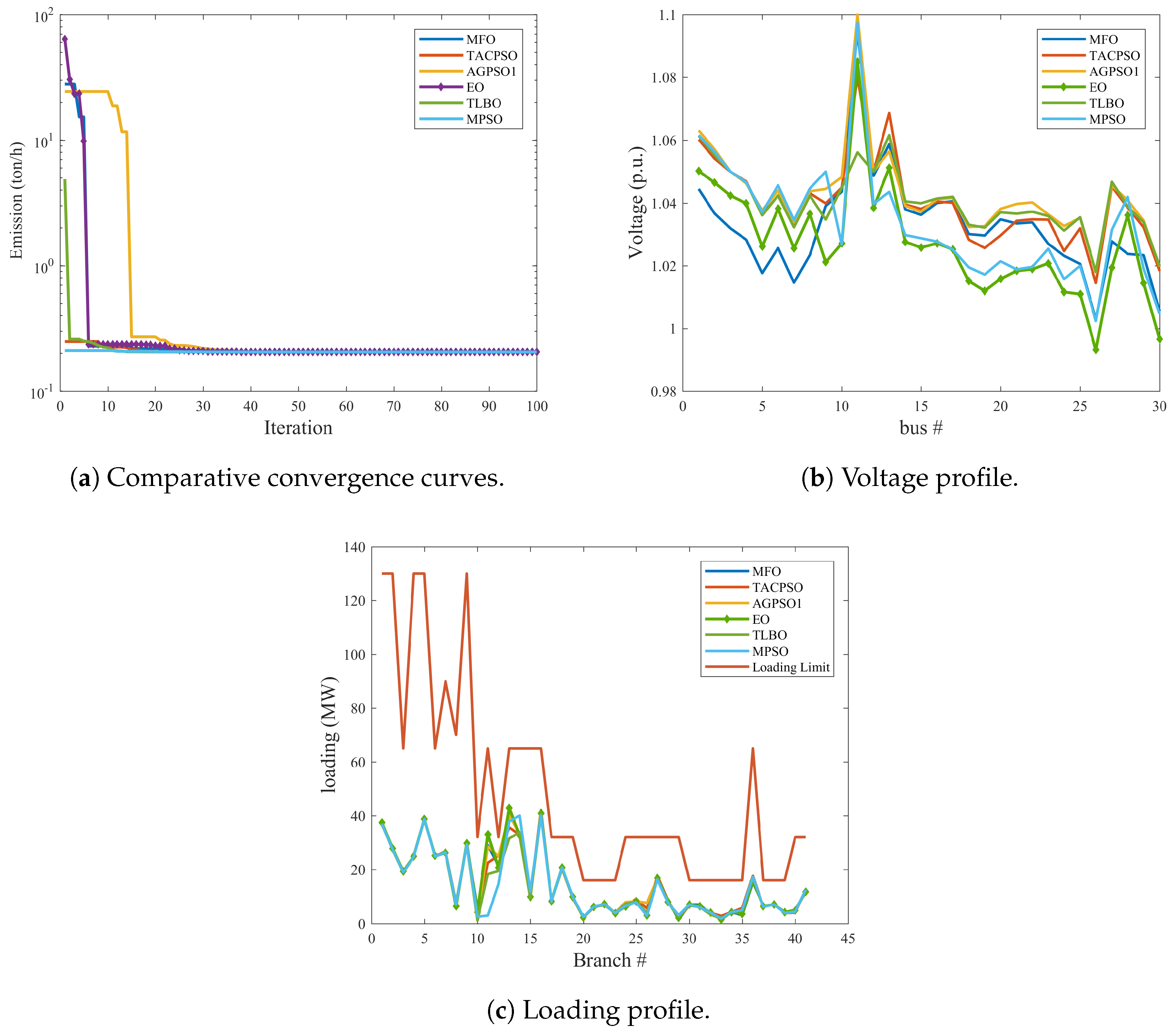
6.1.2. Emission Index Minimization
6.1.3. Minimization of the Total Cost of Generating Units
6.1.4. Voltage Deviation Minimization
6.1.5. Case 5: Minimization of the Total Cost of the Generating Units, Voltage Deviation, Real Power Loss, and Emission Index
7. Conclusions
Author Contributions
Funding
Conflicts of Interest
Abbreviations
| OPF | Optimal power flow |
| NLP | Continuous nonlinear programming |
| PCIP | Predictor-corrector interior point algorithm |
| PSO | Particle swarm optimization |
| QP | Quadratic programming |
| SQP | Sequential quadratic programming |
| MILP | Mixed-integer linear programming |
| TLBO | Teaching–learning-based optimization |
| GSA | Gravitational search algorithm |
| DE | Differential evolution algorithm |
| MTLBO | Modified teaching learning-based optimization algorithm |
| MABC | Fuzzy-based modified bee colony |
| BSO | Brain storming optimization |
| GWO | Grey wolf optimization algorithm |
| EO | Equilibrium optimizer algorithm |
| FACTS | Flexible alternating current transmission system |
References
- Roy, R.; Jadhav, H. Optimal power flow solution of power system incorporating stochastic wind power using Gbest guided artificial bee colony algorithm. Int. J. Electr. Power Energy Syst. 2015, 64, 562–578. [Google Scholar] [CrossRef]
- Shi, L.; Wang, C.; Yao, L.; Ni, Y.; Bazargan, M. Optimal power flow solution incorporating wind power. IEEE Syst. J. 2011, 6, 233–241. [Google Scholar] [CrossRef]
- Biswas, P.P.; Suganthan, P.N.; Mallipeddi, R.; Amaratunga, G.A. Optimal reactive power dispatch with uncertainties in load demand and renewable energy sources adopting scenario-based approach. Appl. Soft Comput. 2019, 75, 616–632. [Google Scholar] [CrossRef]
- Biswas, P.P.; Suganthan, P.; Amaratunga, G.A. Optimal power flow solutions incorporating stochastic wind and solar power. Energy Convers. Manag. 2017, 148, 1194–1207. [Google Scholar] [CrossRef]
- Dommel, H.; Tinney, W. Optimal power flow solutions. IEEE Trans. Power Appar. Syst. 1968, PAS-87, 1866–1876. [Google Scholar] [CrossRef]
- Jabr, R.A. Optimal power flow using an extended conic quadratic formulation. IEEE Trans. Power Syst. 2008, 23, 1000–1008. [Google Scholar] [CrossRef]
- Lin, W.M.; Huang, C.H.; Zhan, T.S. A hybrid current-power optimal power flow technique. IEEE Trans. Power Syst. 2008, 23, 177–185. [Google Scholar] [CrossRef]
- Glavitsch, H.; Spoerry, M. Quadratic loss formula for reactive dispatch. IEEE Trans. Power Appar. Syst. 1983, PAS-102, 3850–3858. [Google Scholar] [CrossRef]
- Burchett, R.; Happ, H.; Wirgau, K. Large scale optimal power flow. IEEE Trans. Power Appar. Syst. 1982, PAS-101, 3722–3732. [Google Scholar] [CrossRef]
- Lobato, E.; Rouco, L.; Navarrete, M.; Casanova, R.; Lopez, G. An LP-based optimal power flow for transmission losses and generator reactive margins minimization. In Proceedings of the 2001 IEEE Porto Power Tech Proceedings (Cat. No. 01EX502), Porto, Portugal, 10–13 September 2001; Volume 3. 5p. [Google Scholar]
- Duman, S.; Güvenç, U.; Sönmez, Y.; Yörükeren, N. Optimal power flow using gravitational search algorithm. Energy Convers. Manag. 2012, 59, 86–95. [Google Scholar] [CrossRef]
- El Ela, A.A.; Abido, M.; Spea, S. Optimal power flow using differential evolution algorithm. Electr. Power Syst. Res. 2010, 80, 878–885. [Google Scholar] [CrossRef]
- Bouchekara, H. Optimal power flow using black-hole-based optimization approach. Appl. Soft Comput. 2014, 24, 879–888. [Google Scholar] [CrossRef]
- Mohamed, A.A.A.; Mohamed, Y.S.; El-Gaafary, A.A.; Hemeida, A.M. Optimal power flow using moth swarm algorithm. Electr. Power Syst. Res. 2017, 142, 190–206. [Google Scholar] [CrossRef]
- Hazra, J.; Sinha, A. A multi-objective optimal power flow using particle swarm optimization. Eur. Trans. Electr. Power 2011, 21, 1028–1045. [Google Scholar] [CrossRef]
- Bhattacharya, A.; Roy, P. Solution of multi-objective optimal power flow using gravitational search algorithm. IET Gener. Transm. Distrib. 2012, 6, 751–763. [Google Scholar] [CrossRef]
- Shabanpour-Haghighi, A.; Seifi, A.R.; Niknam, T. A modified teaching–learning based optimization for multi-objective optimal power flow problem. Energy Convers. Manag. 2014, 77, 597–607. [Google Scholar] [CrossRef]
- Kumar, S.; Chaturvedi, D. Optimal power flow solution using fuzzy evolutionary and swarm optimization. Int. J. Electr. Power Energy Syst. 2013, 47, 416–423. [Google Scholar] [CrossRef]
- Khorsandi, A.; Hosseinian, S.; Ghazanfari, A. Modified artificial bee colony algorithm based on fuzzy multi-objective technique for optimal power flow problem. Electr. Power Syst. Res. 2013, 95, 206–213. [Google Scholar] [CrossRef]
- Ghasemi, M.; Ghavidel, S.; Ghanbarian, M.M.; Gharibzadeh, M.; Vahed, A.A. Multi-objective optimal power flow considering the cost, emission, voltage deviation and power losses using multi-objective modified imperialist competitive algorithm. Energy 2014, 78, 276–289. [Google Scholar] [CrossRef]
- Narimani, M.R.; Azizipanah-Abarghooee, R.; Zoghdar-Moghadam-Shahrekohne, B.; Gholami, K. A novel approach to multi-objective optimal power flow by a new hybrid optimization algorithm considering generator constraints and multi-fuel type. Energy 2013, 49, 119–136. [Google Scholar] [CrossRef]
- Ghasemi, M.; Ghavidel, S.; Akbari, E.; Vahed, A.A. Solving non-linear, non-smooth and non-convex optimal power flow problems using chaotic invasive weed optimization algorithms based on chaos. Energy 2014, 73, 340–353. [Google Scholar] [CrossRef]
- Krishnanand, K.; Hasani, S.M.F.; Panigrahi, B.K.; Panda, S.K. Optimal power flow solution using self-evolving brain-storming inclusive teaching-learning—Based algorithm. In Proceedings of the International Conference in Swarm Intelligence, Harbin, China, 12–15 June 2013; Springer: Berlin/Heidelberg, Germany, 2013. [Google Scholar]
- Sivasubramani, S.; Swarup, K. Sequential quadratic programming based differential evolution algorithm for optimal power flow problem. IET Gener. Transm. Distrib. 2011, 5, 1149–1154. [Google Scholar] [CrossRef]
- Reddy, S.S. Optimal power flow with renewable energy resources including storage. Electr. Eng. 2017, 99, 685–695. [Google Scholar] [CrossRef]
- Shilaja, C.; Arunprasath, T. Optimal power flow using Moth Swarm Algorithm with Gravitational Search Algorithm considering wind power. Future Gener. Comput. Syst. 2019, 98, 708–715. [Google Scholar]
- Aien, M.; Fotuhi-Firuzabad, M.; Rashidinejad, M. Probabilistic optimal power flow in correlated hybrid wind–photovoltaic power systems. IEEE Trans. Smart Grid 2014, 5, 130–138. [Google Scholar] [CrossRef]
- Aien, M.; Rashidinejad, M.; Firuz-Abad, M.F. Probabilistic optimal power flow in correlated hybrid wind-PV power systems: A review and a new approach. Renew. Sustain. Energy Rev. 2015, 41, 1437–1446. [Google Scholar] [CrossRef]
- Liang, R.H.; Tsai, S.R.; Chen, Y.T.; Tseng, W.T. Optimal power flow by a fuzzy based hybrid particle swarm optimization approach. Electr. Power Syst. Res. 2011, 81, 1466–1474. [Google Scholar] [CrossRef]
- Shilaja, C.; Ravi, K. Optimal power flow using hybrid DA-APSO algorithm in renewable energy resources. Energy Procedia 2017, 117, 1085–1092. [Google Scholar] [CrossRef]
- Das, T.; Roy, R.; Mandal, K.K.; Mondal, S.; Mondal, S.; Hait, P.; Das, M.K. Optimal Reactive Power Dispatch Incorporating Solar Power Using Jaya Algorithm. In Computational Advancement in Communication Circuits and Systems; Springer: Berlin/Heidelberg, Germany, 2020; pp. 37–48. [Google Scholar]
- Chen, M.R.; Zeng, G.Q.; Lu, K.D. Constrained multi-objective population extremal optimization based economic-emission dispatch incorporating renewable energy resources. Renew. Energy 2019, 143, 277–294. [Google Scholar] [CrossRef]
- Rambabu, M.; Nagesh Kumar, G.; Sivanagaraju, S. Optimal Power Flow of Integrated Renewable Energy System using a Thyristor Controlled Series Compensator and a Grey-Wolf Algorithm. Energies 2019, 12, 2215. [Google Scholar] [CrossRef]
- Faramarzi, A.; Heidarinejad, M.; Stephens, B.; Mirjalili, S. Equilibrium optimizer: A novel optimization algorithm. Knowl. Based Syst. 2019, 195, 105190. [Google Scholar] [CrossRef]
- Biswas, P.P.; Suganthan, P.N.; Mallipeddi, R.; Amaratunga, G.A. Optimal power flow solutions using differential evolution algorithm integrated with effective constraint handling techniques. Eng. Appl. Artif. Intell. 2018, 68, 81–100. [Google Scholar] [CrossRef]
- Shaheen, A.M.; El-Sehiemy, R.A.; Farrag, S.M. Solving multi-objective optimal power flow problem via forced initialised differential evolution algorithm. IET Gener. Transm. Distrib. 2016, 10, 1634–1647. [Google Scholar] [CrossRef]
- Panda, A.; Tripathy, M. Security constrained optimal power flow solution of wind-thermal generation system using modified bacteria foraging algorithm. Energy 2015, 93, 816–827. [Google Scholar] [CrossRef]
- Shargh, S.; Mohammadi-Ivatloo, B.; Seyedi, H.; Abapour, M. Probabilistic multi-objective optimal power flow considering correlated wind power and load uncertainties. Renew. Energy 2016, 94, 10–21. [Google Scholar] [CrossRef]
- Biswas, P.P.; Suganthan, P.N.; Qu, B.Y.; Amaratunga, G.A. Multiobjective economic-environmental power dispatch with stochastic wind-solar-small hydro power. Energy 2018, 150, 1039–1057. [Google Scholar] [CrossRef]
- Hu, F.; Hughes, K.J.; Ma, L.; Pourkashanian, M. Combined economic and emission dispatch considering conventional and wind power generating units. Int. Trans. Electr. Energy Syst. 2017, 27, e2424. [Google Scholar] [CrossRef]
- Hu, F.; Hughes, K.J.; Ingham, D.B.; Ma, L.; Pourkashanian, M. Dynamic economic and emission dispatch model considering wind power under Energy Market Reform: A case study. Int. J. Electr. Power Energy Syst. 2019, 110, 184–196. [Google Scholar] [CrossRef]
- Taha, I.B.; Elattar, E.E. Optimal reactive power resources sizing for power system operations enhancement based on improved grey wolf optimiser. IET Gener. Transm. Distrib. 2018, 12, 3421–3434. [Google Scholar] [CrossRef]
- Alsac, O.; Stott, B. Optimal load flow with steady-state security. IEEE Trans. Power Appar. Syst. 1974, PAS-93, 745–751. [Google Scholar] [CrossRef]
- Zimmerman, R.D.; Murillo-Sánchez, C.E.; Gan, D. MATPOWER: A MATLAB power system simulation package. Manual Power Syst. Eng. Res. Center Ithaca NY 1997, 1, 8–38. [Google Scholar]
- Mirjalili, S.; Lewis, A.; Sadiq, A.S. Autonomous particles groups for particle swarm optimization. Arab. J. Sci. Eng. 2014, 39, 4683–4697. [Google Scholar] [CrossRef]
- Rao, R.V.; Savsani, V.J.; Vakharia, D. Teaching—Learning-based optimization: An optimization method for continuous non-linear large scale problems. Inf. Sci. 2012, 183, 1–15. [Google Scholar] [CrossRef]
- Mirjalili, S. Moth-flame optimization algorithm: A novel nature-inspired heuristic paradigm. Knowl. Based Syst. 2015, 89, 228–249. [Google Scholar] [CrossRef]


| Generator | Bus | |||||
|---|---|---|---|---|---|---|
| G1 | 1 | 4.091 | −5.554 | 6.49 | 0.0002 | 2.857 |
| G2 | 2 | 2.543 | −6.047 | 5.638 | 0.0005 | 3.333 |
| G3 | 5 | 4.258 | −5.094 | 4.586 | 0.000001 | 8 |
| G4 | 8 | 5.326 | −3.55 | 3.38 | 0.002 | 2 |
| G5 | 11 | 4.258 | −5.094 | 4.586 | 0.000001 | 8 |
| G6 | 13 | 6.131 | −5.555 | 5.151 | 0.00001 | 6.667 |
| Generator | Bus | a | b | c |
|---|---|---|---|---|
| G1 | 1 | 0 | 2 | 0.00375 |
| G2 | 2 | 0 | 1.75 | 0.0175 |
| G3 | 5 | 0 | 1 | 0.0625 |
| G4 | 8 | 0 | 3.25 | 0.00834 |
| G5 | 11 | 0 | 3 | 0.025 |
| G6 | 13 | 0 | 3 | 0.025 |
| Values and Details | ||||
|---|---|---|---|---|
| Characteristics | Test System 1 [42,43,44] | Test System 2 | Test System 3 | Test System 4 |
| Buses | 30 | 30 | 30 | 30 |
| Transmission Lines | 41 | 41 | 41 | 41 |
| Limitation on generator voltage | [0.9–1.1] | [0.9–1.1] | [0.9–1.1] | [0.9–1.1] |
| Limitation on load voltage | [0.95–1.1] | [0.95–1.1] | [0.95–1.1] | [0.95–1.1] |
| Thermal power generators | 6 | 3 | 3 | 3 |
| Wind power plants | 0 | 2 | 0 | 5 |
| Solar power plants | 0 | 3 | 5 | 0 |
| Shunt VAR compensation | 9 | 9 | 9 | 9 |
| Transformer with tap ratio | 4 | 4 | 4 | 4 |
| Control Variables | 24 | 28 | 28 | 28 |
| Active and Reactive power demand | 283.4 MW, 126.2 Mvar | 283.4 MW, 126.2 Mvar | 283.4 MW, 126.2 Mvar | 283.4 MW, 126.2 Mvar |
| Unit | Bus | No. of Turbines | [MW] | k | c | [$/MWH] | [$/MWH] | [$/MWH] | [m/s] | [m/s] | [m/s] |
|---|---|---|---|---|---|---|---|---|---|---|---|
| 1 | 11 | 12 | 2 | 2 | 9 | 1.7 | 2.8 | 1.7 | 4 | 25 | 13 |
| 2 | 30 | 12 | 2 | 2 | 10 | 1.7 | 2.8 | 1.7 | 4 | 25 | 13 |
| Unit | Bus | [MW] | [W/m] | [W/m] | [$/MWh] | [$/MWh] | [$/MWh] | ||
|---|---|---|---|---|---|---|---|---|---|
| 1 | 5 | 24 | 800 | 170 | 6 | 0.6 | 1.55 | 3.2 | 1.30 |
| 2 | 13 | 30 | 800 | 170 | 6 | 0.6 | 1.45 | 3.1 | 1.45 |
| 3 | 30 | 30 | 800 | 200 | 6 | 0.6 | 1.60 | 3.0 | 1.30 |
| Unit | Bus | [MW] | [W/m] | [W/m] | [$/MWh] | [$/MWh] | [$/MWh] | ||
|---|---|---|---|---|---|---|---|---|---|
| 1 | 5 | 24 | 800 | 170 | 6 | 0.6 | 1.55 | 3.2 | 1.30 |
| 2 | 11 | 24 | 800 | 200 | 6 | 0.6 | 1.45 | 2.8 | 1.30 |
| 3 | 13 | 24 | 800 | 170 | 6 | 0.6 | 1.60 | 3.1 | 1.45 |
| 4 | 24 | 30 | 800 | 170 | 6 | 0.6 | 1.60 | 3.0 | 1.30 |
| 5 | 30 | 30 | 800 | 200 | 6 | 0.6 | 1.60 | 3.0 | 1.30 |
| Unit | Bus | No. of Turbines | [MW] | k | c | [$/MWH] | [$/MWH] | [$/MWH] | [m/s] | [m/s] | [m/s] |
|---|---|---|---|---|---|---|---|---|---|---|---|
| 1 | 5 | 12 | 2 | 2 | 9 | 1.65 | 2.6 | 1.5 | 4 | 25 | 13 |
| 2 | 11 | 12 | 2 | 2 | 10 | 1.60 | 2.6 | 1.5 | 4 | 25 | 13 |
| 3 | 13 | 12 | 2 | 2 | 9 | 1.60 | 2.6 | 1.5 | 4 | 25 | 13 |
| 4 | 24 | 15 | 2 | 2 | 10 | 1.65 | 2.6 | 1.5 | 4 | 25 | 13 |
| 5 | 30 | 15 | 2 | 2 | 9 | 1.70 | 2.6 | 1.5 | 4 | 25 | 13 |
| Algorithm | Parameters | Values |
|---|---|---|
| MPSO [45] | Inertia coefficient (w) | decreasing linearly from 0.9 to 0.4 |
| Number of search agents | 50 | |
| Maximum number of iteration | 100 | |
| Udapting factor (C1,C2) | Described in [45] | |
| Acceleration coefficient (c1,c2) | c1 = 1, c2 = 2 | |
| TLBO [46] | Teaching factor | Selected randomly [1,2] |
| Population size | 50 | |
| Maximum number of iteration | 100 | |
| TACPSO [45] | Inertia coefficient (w) | decreasing linearly from 0.9 to 0.4 |
| Number of search agents | 50 | |
| Maximum number of iteration | 100 | |
| Udapting factor (C1,C2) | Described in [45] | |
| Acceleration coefficient (c1,c2) | c1 = 1, c2 = 2 | |
| MFO [47] | Population size | 50 |
| Maximum number of iteration | 100 | |
| Shape constant (b) | 1 | |
| AGPSO 1 [45] | Inertia coefficient (w) | decreasing linearly from 0.9 to 0.4 |
| Number of search agents | 50 | |
| Maximum number of iteration | 100 | |
| Udapting factor (C1,C2) | Described in [45] | |
| Acceleration coefficient (c1,c2) | c1 = 1, c2 = 2 | |
| EO [34] | Constant values for controlling exploration () | 2 |
| Constant values for controlling exploitation () | 1 | |
| Number of search particles | 50 | |
| Maximum number of iteration | 100 | |
| Generation probability | 0.5 |
| MFO | TACPSO | AGPSO1 | TLBO | EO | MPSO | |
|---|---|---|---|---|---|---|
| (p.u.) | 0.867649 | 0.898003 | 0.898362 | 0.87350728 | 0.917249 | 0.679794 |
| ($/h) | 967.4482 | 967.6206 | 967.6485 | 967.2492825 | 967.5865 | 967.7676 |
| (MW) | 3.124412 | 3.100891 | 3.094156 | 3.108417583 | 3.087342 | 3.144079 |
| E (ton/h) | 0.207299 | 0.207259 | 0.207266 | 0.207286164 | 0.207268 | 0.207273 |
| 3.124412 | 3.100891 | 3.094156 | 3.108417583 | 3.087342 | 3.144079 | |
| 1.18 | 0.43 | 0.22 | 0.68 | - | 1.81 |
| Parameters | Min | Max | Test System 1 | Test System 2 | Test System 3 | Test System 4 |
|---|---|---|---|---|---|---|
| PG2 (MW) | 20 | 80 | 79.9983006 | 72.14028714 | 48.22886744 | 51.07651611 |
| PG5 (MW) | 15 | 50 | 49.9982627 | 49.99945385 | 49.97347066 | 49.98470056 |
| PG8 (MW) | 10 | 35 | 34.99453958 | 26.20234283 | 34.77838714 | 34.92764479 |
| PG11 (MW) | 10 | 30 | 29.99984469 | 29.42347144 | 29.97517159 | 29.67713532 |
| PG13 (MW) | 10 | 40 | 39.99027741 | 25.72695297 | 29.69711674 | 39.69895071 |
| PG24 (MW) | 10 | 30 | 18.61010237 | 27.4148297 | 15.73782289 | |
| PG30 (MW) | 10 | 40 | 13.58641689 | 15.23102984 | 14.35575851 | |
| V1 (p.u.) | 0.95 | 1.1 | 1.061430345 | 1.033582214 | 1.037749499 | 1.056224426 |
| V2 (p.u.) | 0.95 | 1.1 | 1.057379791 | 1.027683624 | 1.032739079 | 1.051241045 |
| V5 (p.u.) | 0.95 | 1.1 | 1.037622078 | 1.003632229 | 1.013755431 | 1.032812731 |
| V8 (p.u.) | 0.95 | 1.1 | 1.044007621 | 1.015022765 | 1.02707043 | 1.045463882 |
| V11 (p.u.) | 0.95 | 1.1 | 1.073279794 | 1.063216144 | 0.999050197 | 1.042867188 |
| V13 (p.u.) | 0.95 | 1.1 | 1.051619936 | 1.034701938 | 1.044856898 | 1.020563172 |
| V24 (p.u.) | 0.95 | 1.1 | 1.024480465 | 1.009002895 | 1.020352939 | |
| V30 (p.u.) | 0.95 | 1.1 | 1.022453184 | 1.018925985 | 1.040981535 | |
| QC10 (MVAr) | 0 | 5 | 4.287709826 | 4.782286758 | 2.62406261 | 3.612693403 |
| QC12 (MVAr) | 0 | 5 | 2.093601675 | 0.000803534 | 0.986423834 | 2.416935212 |
| QC15 (MVAr) | 0 | 5 | 3.996488379 | 1.898614523 | 0.206692775 | 3.600783886 |
| QC17 (MVAr) | 0 | 5 | 4.136235738 | 4.356883849 | 2.716911629 | 0.342465282 |
| QC20 (MVAr) | 0 | 5 | 4.495134896 | 3.354513668 | 4.692404829 | 3.296807199 |
| QC21 (MVAr) | 0 | 5 | 5.000000000 | 0.046094293 | 2.038284465 | 0.872744865 |
| QC23 (MVAr) | 0 | 5 | 3.197386977 | 4.967912056 | 4.957773966 | 4.740324068 |
| QC24 (MVAr) | 0 | 5 | 4.806462479 | 4.536993047 | 3.79952116 | 3.698494945 |
| QC29 (MVAr) | 0 | 5 | 2.461175597 | 0.21865228 | 4.63994E−05 | 3.927880442 |
| T11 (p.u.) | 0.9 | 1.1 | 1.055740955 | 1.015687471 | 1.020034326 | 1.0962353 |
| T12 (p.u.) | 0.9 | 1.1 | 0.924042761 | 0.951998195 | 0.957069803 | 0.900424717 |
| T15 (p.u.) | 0.9 | 1.1 | 0.988530694 | 0.989254661 | 1.094558386 | 0.991494831 |
| T36 (p.u.) | 0.9 | 1.1 | 0.975749345 | 0.977273155 | 1.010207101 | 1.010623787 |
| PG1 (MW) | 50 | 200 | 51.50611659 | 50.08572807 | 50.22954768 | 50.01396753 |
| QG1 (MVAr) | −20 | 150 | −5.485983591 | −1.712627012 | −9.408754457 | −4.363894439 |
| QG2 (MVAr) | −20 | 60 | 7.574416698 | 7.129014137 | 3.920290677 | 9.504062082 |
| QG5 (MVAr) | −15 | 62.5 | 21.13271229 | 17.01446382 | 19.68757038 | 20.6489489 |
| QG8 (MVAr) | −15 | 48 | 26.41312254 | 26.16274206 | 28.52016815 | 33.06577869 |
| QG11 (MVAr) | −10 | 40 | 19.21231862 | 19.38101083 | 0.13383456 | 18.93870787 |
| QG13 (MVAr) | −15 | 44 | 2.247530335 | 8.029799729 | 33.49981989 | −2.320248965 |
| QG24 (MVAr) | −15 | 44 | 3.105401958 | 3.720374455 | 2.56415683 | |
| QG 30 (MVAr) | −15 | 44 | 0.296246809 | 2.993820748 | 1.368798025 | |
| (p.u.) | 0.917249187 | 0.367181831 | 0.252949566 | 0.482190403 | ||
| ($/h) | 967.5864625 | 417.7815499 | 358.1435956 | 368.1354088 | ||
| (MW) | 3.087341565 | 2.374755583 | 2.128420834 | 2.072496662 | ||
| E (ton/h) | 0.20726839 | 0.09655031 | 0.09111361 | 0.091202895 | ||
| ($/h) | 863.2203104 | 823.476285 | 867.8385329 | |||
| ($/h) | 141.4837171 | 499.7031241 | ||||
| ($/h) | 303.9550435 | 465.3326895 | ||||
| (MW) | 3.087341565 | 2.374755583 | 2.128420834 | 2.072496662 |
| Best | Worst | Mean | Std dev | |
|---|---|---|---|---|
| MFO | 3.124412 | 3.469255 | 3.313791 | 0.115148 |
| TACPSO | 3.100891 | 3.495604 | 3.162984 | 0.119564 |
| AGPSO1 | 3.094156 | 3.558659 | 3.136808 | 0.175963 |
| TLBO | 3.108418 | 3.271804 | 3.200392 | 0.057571 |
| EO | 3.087342 | 3.131426 | 3.089549 | 0.013218 |
| MPSO | 3.144079 | 3.417325 | 3.202598 | 0.080901 |
| Parameters | Min | Max | Test System 1 | Test System 2 | Test System 3 | Test System 4 |
|---|---|---|---|---|---|---|
| PG2 (MW) | 20 | 80 | 67.52765352 | 47.15393481 | 46.93784062 | 46.74579811 |
| PG5 (MW) | 15 | 50 | 49.99976843 | 49.99997692 | 48.55695793 | 49.63943974 |
| PG8 (MW) | 10 | 35 | 34.99979715 | 34.99785564 | 35.00000000 | 34.99981323 |
| PG11 (MW) | 10 | 30 | 30.00000000 | 13.08937369 | 24.11263394 | 28.93951933 |
| PG13 (MW) | 10 | 40 | 39.99994042 | 39.97364116 | 38.90979918 | 31.15977654 |
| PG24 (MW) | 10 | 30 | 29.67649489 | 20.72363213 | 13.68967898 | |
| PG30 (MW) | 10 | 40 | 22.06349364 | 22.1793691 | 32.00183302 | |
| V1 (p.u.) | 0.95 | 1.1 | 1.061391900 | 1.035577033 | 1.017785294 | 1.007633877 |
| V2 (p.u.) | 0.95 | 1.1 | 1.055299891 | 1.03014784 | 1.009596473 | 0.99225379 |
| V5 (p.u.) | 0.95 | 1.1 | 1.036061646 | 0.975474909 | 0.982885915 | 0.966515297 |
| V8 (p.u.) | 0.95 | 1.1 | 1.042336524 | 0.994262522 | 0.996877809 | 0.970873143 |
| V11 (p.u.) | 0.95 | 1.1 | 1.056098162 | 0.99155371 | 1.066472978 | 1.018197794 |
| V13 (p.u.) | 0.95 | 1.1 | 1.061630874 | 1.045591502 | 1.053301428 | 0.990382535 |
| V24 (p.u.) | 0.95 | 1.1 | 0.994310052 | 1.023161602 | 1.006430427 | |
| V30 (p.u.) | 0.95 | 1.1 | 0.976743321 | 0.962066536 | 0.995194145 | |
| QC10 (MVAr) | 0 | 5 | 4.194820255 | 0.691891638 | 0.00000000 | 2.28917862 |
| QC12 (MVAr) | 0 | 5 | 0.527663733 | 3.89808945 | 4.781805725 | 0.003693677 |
| QC15 (MVAr) | 0 | 5 | 4.925786364 | 0.093781976 | 4.681393138 | 3.767863825 |
| QC17 (MVAr) | 0 | 5 | 4.982842903 | 2.766984513 | 4.998326488 | 4.887538377 |
| QC20 (MVAr) | 0 | 5 | 4.671024822 | 4.426843395 | 4.610963598 | 5.000000000 |
| QC21 (MVAr) | 0 | 5 | 4.976075346 | 1.329009086 | 4.940763823 | 2.759967479 |
| QC23 (MVAr) | 0 | 5 | 2.74762835 | 3.54838243 | 0.002439547 | 4.271161763 |
| QC24 (MVAr) | 0 | 5 | 4.992557282 | 0.606928317 | 0.970384621 | 2.50397663 |
| QC29 (MVAr) | 0 | 5 | 2.088379542 | 4.949034272 | 0.000438444 | 2.957731038 |
| T11 (p.u.) | 0.9 | 1.1 | 1.045594251 | 0.951879814 | 0.938502294 | 0.940072546 |
| T12 (p.u.) | 0.9 | 1.1 | 0.921878284 | 0.962206441 | 1.096587454 | 0.919312335 |
| T15 (p.u.) | 0.9 | 1.1 | 1.00248085 | 1.099174642 | 1.018026147 | 1.023627655 |
| T36 (p.u.) | 0.9 | 1.1 | 0.972355171 | 0.92579926 | 1.099689643 | 1.060629423 |
| PG1 (MW) | 50 | 200 | 64.09434175 | 50.00003511 | 50.00023516 | 50.00000501 |
| QG1 (MVAr) | −20 | 150 | −5.544691231 | 0.054641352 | −1.33241509 | 18.58616272 |
| QG2 (MVAr) | −20 | 60 | 6.45002148 | 47.44923402 | 4.202024706 | 1.97952536 |
| QG5 (MVAr) | −15 | 62.5 | 21.67156016 | −1.442938766 | 13.43474762 | 19.83503047 |
| QG8 (MVAr) | −15 | 48 | 27.29675405 | 23.11453954 | 7.583267029 | 12.95707181 |
| QG11 (MVAr) | −10 | 40 | 11.72500454 | −6.137543909 | 13.66528344 | 1.654000716 |
| QG13 (MVAr) | −15 | 44 | 9.840166661 | 39.23629311 | 21.68524583 | 6.151027816 |
| QG24 (MVAr) | −15 | 44 | 1.089772208 | 24.29742231 | 20.10756016 | |
| QG 30 (MVAr) | −15 | 44 | −13.49116551 | 0.162345045 | 0.721702425 | |
| (p.u.) | 0.90040310 | 0.298468513 | 0.404641642 | 0.391340877 | ||
| ($/h) | 944.2808599 | 354.7638857 | 354.038595 | 353.3864113 | ||
| (MW) | 3.22150126 | 3.554805885 | 3.020468191 | 3.775864192 | ||
| E (ton/h) | 0.204818699 | 0.091061921 | 0.091060623 | 0.091060048 | ||
| ($/h) | 877.5739313 | 865.4758094 | 867.8663197 | |||
| ($/h) | 108.3986993 | 514.4799085 | ||||
| ($/h) | 414.4113463 | 511.4372144 | ||||
| (ton/h) | 0.204818699 | 0.091061921 | 0.091060623 | 0.091060048 |
| MFO | TACPSO | AGPSO1 | TLBO | EO | MPSO | |
|---|---|---|---|---|---|---|
| (p.u.) | 0.702001 | 0.856848 | 0.921129 | 0.541768425 | 0.900403 | 0.661504 |
| ($/h) | 944.3434 | 944.6554 | 944.3977 | 944.6873755 | 944.2809 | 944.4382 |
| (MW) | 3.356033 | 3.286856 | 3.235581 | 3.336091467 | 3.221501 | 3.267419 |
| E (ton/h) | 0.204862 | 0.204839 | 0.204823 | 0.204854728 | 0.204819 | 0.204833 |
| (ton/h) | 0.204862 | 0.204839 | 0.204823 | 0.204854728 | 0.204819 | 0.204833 |
| Best | Worst | Mean | Std Dev | |
|---|---|---|---|---|
| MFO | 0.204862 | 0.204997 | 0.20495 | 4.15 × 10 |
| TACPSO | 0.204839 | 0.205089 | 0.204943 | 9.14 × 10 |
| AGPSO1 | 0.204823 | 0.204999 | 0.204921 | 5.14 × 10 |
| TLBO | 0.204855 | 0.204931 | 0.204892 | 2.43 × 10 |
| EO | 0.204819 | 0.204878 | 0.204834 | 1.78 × 10 |
| MPSO | 0.204833 | 0.20497 | 0.204934 | 5.44 × 10 |
| MFO | TACPSO | AGPSO1 | TLBO | EO | MPSO | |
|---|---|---|---|---|---|---|
| (p.u.) | 0.740965 | 0.845878 | 0.761669 | 0.811019872 | 0.865075 | 0.877139 |
| ($/h) | 800.8283 | 800.5201 | 800.5595 | 800.616176 | 800.4486 | 800.5346 |
| (MW) | 9.134902 | 9.02898 | 9.040104 | 8.97569702 | 9.041464 | 9.059254 |
| E (ton/h) | 0.366492 | 0.366315 | 0.365967 | 0.363482104 | 0.367478 | 0.366949 |
| ($/h) | 800.8283 | 800.5201 | 800.5595 | 800.616176 | 800.4486 | 800.5346 |
| Best | Worst | Mean | Std Dev | |
|---|---|---|---|---|
| MFO | 800.8283 | 802.8078 | 801.5102 | 0.72899 |
| TACPSO | 800.5201 | 804.0448 | 800.6766 | 1.305504 |
| AGPSO1 | 800.5595 | 802.1145 | 800.7023 | 0.453581 |
| TLBO | 800.6162 | 802.225 | 800.8366 | 0.471362 |
| EO | 800.4486 | 800.646 | 800.4793 | 0.057894 |
| MPSO | 800.5346 | 804.6442 | 801.1155 | 1.810857 |
| Parameters | Min | Max | Test System 1 | Test System 2 | Test System 3 | Test System 4 |
|---|---|---|---|---|---|---|
| PG2 (MW) | 20 | 80 | 48.74605575 | 45.18712121 | 21.21838812 | 38.17119779 |
| PG5 (MW) | 15 | 50 | 21.4315437 | 15.00195728 | 15.40668673 | 19.095538 |
| PG8 (MW) | 10 | 35 | 21.18353338 | 29.97018297 | 15.60913424 | 10.08641797 |
| PG11 (MW) | 10 | 30 | 11.52952165 | 13.07275916 | 29.402226 | 20.7452611 |
| PG13 (MW) | 10 | 40 | 12.0107829 | 19.71387022 | 30.51540057 | 17.9328134 |
| PG24 (MW) | 10 | 30 | 27.19702311 | 26.3304831 | 25.32965431 | |
| PG30 (MW) | 10 | 40 | 14.74139467 | 17.72178713 | 20.28023584 | |
| V1 (p.u.) | 0.95 | 1.1 | 1.081191705 | 1.022713246 | 1.02314065 | 1.059255936 |
| V2 (p.u.) | 0.95 | 1.1 | 1.063110135 | 1.006065736 | 1.008766945 | 1.043719467 |
| V5 (p.u.) | 0.95 | 1.1 | 1.032684857 | 0.956733982 | 0.961917138 | 1.009460201 |
| V8 (p.u.) | 0.95 | 1.1 | 1.036543249 | 0.994159517 | 0.985269141 | 1.02095678 |
| V11 (p.u.) | 0.95 | 1.1 | 1.097591909 | 1.012587735 | 1.049992902 | 1.0845661 |
| V13 (p.u.) | 0.95 | 1.1 | 1.051244633 | 1.054638289 | 1.011514979 | 1.046208927 |
| V24 (p.u.) | 0.95 | 1.1 | 1.035583887 | 1.011800496 | 1.043496784 | |
| V30 (p.u.) | 0.95 | 1.1 | 0.950000000 | 0.996591531 | 1.048407181 | |
| QC10 (MVAr) | 0 | 5 | 2.971616423 | 3.739491269 | 4.902790106 | 0.325756054 |
| QC12 (MVAr) | 0 | 5 | 0.655177618 | 4.809891924 | 1.662706176 | 3.06145818 |
| QC15 (MVAr) | 0 | 5 | 3.197516308 | 0.002648509 | 0.249875162 | 3.301750446 |
| QC17 (MVAr) | 0 | 5 | 4.723716655 | 3.279961844 | 1.827574807 | 1.707154585 |
| QC20 (MVAr) | 0 | 5 | 3.650622268 | 0.917150962 | 1.107119341 | 0.418013886 |
| QC21 (MVAr) | 0 | 5 | 5.000000000 | 4.948708899 | 2.08610321 | 4.893042007 |
| QC23 (MVAr) | 0 | 5 | 2.498554056 | 4.535914953 | 4.240774401 | 3.58924067 |
| QC24 (MVAr) | 0 | 5 | 4.985418463 | 5.000000000 | 0.00000000 | 1.169769378 |
| QC29 (MVAr) | 0 | 5 | 2.584313587 | 4.144114834 | 4.95463484 | 1.500067393 |
| T11 (p.u.) | 0.9 | 1.1 | 1.027284076 | 1.048412041 | 1.099843892 | 0.985023037 |
| T12 (p.u.) | 0.9 | 1.1 | 0.971275895 | 0.90000000 | 0.922169184 | 0.989956238 |
| T15 (p.u.) | 0.9 | 1.1 | 0.972373363 | 1.002944153 | 1.006664961 | 0.991751478 |
| T36 (p.u.) | 0.9 | 1.1 | 0.9815263 | 1.059841992 | 0.944073975 | 0.971316876 |
| PG1 (MW) | 50 | 200 | 177.5400261 | 125.374001 | 133.7249716 | 138.0708394 |
| QG1 (MVAr) | −20 | 150 | −0.570024945 | −0.833938199 | −5.669301771 | −1.647701957 |
| QG2 (MVAr) | −20 | 60 | 19.80925666 | 13.30674022 | 30.0465083 | 18.91158888 |
| QG5 (MVAr) | −15 | 62.5 | 25.58480054 | 6.160576051 | 11.07617293 | 21.00268292 |
| QG8 (MVAr) | −15 | 48 | 23.28431397 | 23.75265502 | 14.5584729 | 21.65678972 |
| QG11 (MVAr) | −10 | 40 | 25.55139519 | 8.157153402 | 35.09222447 | 19.52230631 |
| QG13 (MVAr) | −15 | 44 | 1.335643081 | 21.55072062 | 12.13070192 | 7.287213883 |
| QG24 (MVAr) | −15 | 44 | 22.34214251 | 15.27252587 | 8.101017671 | |
| QG 30 (MVAr) | −15 | 44 | −5.331414964 | −8.278410983 | −1.403218975 | |
| (p.u.) | 0.865074691 | 0.312619858 | 0.288839815 | 0.653856503 | ||
| ($/h) | 800.4486031 | 529.3973749 | 432.2815387 | 473.5571537 | ||
| (MW) | 9.041463508 | 6.858309749 | 6.529077621 | 6.311958209 | ||
| E (ton/h) | 0.367478227 | 0.141650437 | 0.159248156 | 0.163097259 | ||
| ($/h) | 772.2465456 | 772.7810970 | 777.3121394 | |||
| ($/h) | 85.46692162 | 303.7549857 | ||||
| ($/h) | 157.3822491 | 340.4995583 | ||||
| ($/h) | 800.4486031 | 772.2465456 | 772.7810970 | 777.3121394 |
| Parameters | Min | Max | Test System 1 | Test System 2 | Test System 3 | Test System 4 |
|---|---|---|---|---|---|---|
| PG2 (MW) | 20 | 80 | 70.18121441 | 35.84850999 | 73.22346542 | 42.82238053 |
| PG5 (MW) | 15 | 50 | 25.52703119 | 20.27116158 | 33.56379457 | 47.02961201 |
| PG8 (MW) | 10 | 35 | 28.87890546 | 17.61889372 | 18.04097353 | 33.85695266 |
| PG11 (MW) | 10 | 30 | 29.30401557 | 24.63092203 | 10.13966121 | 14.67013887 |
| PG13 (MW) | 10 | 40 | 27.92172576 | 15.28698582 | 21.57955174 | 39.93831108 |
| PG24 (MW) | 10 | 30 | 16.34156919 | 10.07569951 | 28.44997135 | |
| PG30 (MW) | 10 | 40 | 26.43024961 | 24.9797807 | 28.73744876 | |
| V1 (p.u.) | 0.95 | 1.1 | 1.009811989 | 1.032801388 | 1.022207169 | 1.012647301 |
| V2 (p.u.) | 0.95 | 1.1 | 1.003153500 | 1.026505843 | 1.020581934 | 1.004121334 |
| V5 (p.u.) | 0.95 | 1.1 | 1.015213206 | 1.016105476 | 1.019877057 | 1.020275353 |
| V8 (p.u.) | 0.95 | 1.1 | 1.008124785 | 0.993094249 | 0.998231049 | 1.001227396 |
| V11 (p.u.) | 0.95 | 1.1 | 1.038640051 | 1.003641057 | 1.02134836 | 0.99563608 |
| V13 (p.u.) | 0.95 | 1.1 | 1.005894818 | 1.02703208 | 0.996453698 | 1.022325949 |
| V24 (p.u.) | 0.95 | 1.1 | 1.013528762 | 1.014235434 | 1.018656779 | |
| V30 (p.u.) | 0.95 | 1.1 | 1.002929877 | 0.993533496 | 0.998414844 | |
| QC10 (MVAr) | 0 | 5 | 4.999434200 | 1.057601365 | 4.449085771 | 1.224696754 |
| QC12 (MVAr) | 0 | 5 | 4.602398118 | 2.55410853 | 4.99999823 | 2.663316679 |
| QC15 (MVAr) | 0 | 5 | 4.960424711 | 4.999607248 | 1.610176653 | 3.415934203 |
| QC17 (MVAr) | 0 | 5 | 0.01181544 | 0.217347144 | 1.996228043 | 0.019033266 |
| QC20 (MVAr) | 0 | 5 | 4.996883927 | 4.92956648 | 4.978309396 | 4.994054795 |
| QC21 (MVAr) | 0 | 5 | 4.956429831 | 1.646590977 | 0.034134918 | 4.819904248 |
| QC23 (MVAr) | 0 | 5 | 4.972309922 | 0.427048793 | 1.956957345 | 1.039869954 |
| QC24 (MVAr) | 0 | 5 | 4.980435681 | 2.406207968 | 4.614781826 | 0.613094925 |
| QC29 (MVAr) | 0 | 5 | 2.520824595 | 1.71349761 | 3.890942901 | 3.740081954 |
| T11 (p.u.) | 0.9 | 1.1 | 1.056622635 | 1.012874303 | 1.035801681 | 1.002332018 |
| T12 (p.u.) | 0.9 | 1.1 | 0.901402975 | 0.900602964 | 0.902285005 | 0.901103808 |
| T15 (p.u.) | 0.9 | 1.1 | 0.981060937 | 1.013218403 | 0.960787866 | 0.998733169 |
| T36 (p.u.) | 0.9 | 1.1 | 0.966944023 | 0.987755959 | 0.989855906 | 0.98143194 |
| PG1 (MW) | 50 | 200 | 108.1160533 | 133.9296827 | 97.60688393 | 51.45175998 |
| QG1 (MVAr) | −20 | 150 | −19.10239902 | −19.59757178 | −19.11821266 | −0.518817877 |
| QG2 (MVAr) | −20 | 60 | −14.85253038 | 31.85856685 | 18.90601653 | −16.64972076 |
| QG5 (MVAr) | −15 | 62.5 | 57.49581183 | 49.60698522 | 51.42002978 | 56.50571855 |
| QG8 (MVAr) | −15 | 48 | 45.23093447 | 11.80532985 | 26.14354452 | 31.44056819 |
| QG11 (MVAr) | −10 | 40 | 20.12674964 | 2.380585374 | 10.62092072 | −1.914317997 |
| QG13 (MVAr) | −15 | 44 | −1.74441538 | 13.80317636 | −8.465359993 | 10.55389137 |
| QG24 (MVAr) | −15 | 44 | 14.86630972 | 15.99035449 | 13.88576475 | |
| QG 30 (MVAr) | −15 | 44 | −4.888937122 | −7.68659143 | −7.960636408 | |
| (p.u.) | 0.088397534 | 0.08005165 | 0.064632335 | 0.07266919 | ||
| ($/h) | 848.7795548 | 480.1984844 | 514.2584395 | 339.455916 | ||
| (MW) | 6.528945889 | 6.957974748 | 5.809810669 | 3.556575273 | ||
| E (ton/h) | 0.240505607 | 0.155665569 | 0.119726864 | 0.091393798 | ||
| ($/h) | 787.9483007 | 810.1863986 | 861.8303756 | |||
| ($/h) | 164.0403370 | 522.3744597 | ||||
| ($/h) | 143.7094792 | 295.9279591 | ||||
| (p.u.) | 0.088397534 | 0.080051650 | 0.064632335 | 0.07266919 |
| Best | Worst | Mean | Std Dev | |
|---|---|---|---|---|
| MFO | 0.100862 | 0.137899 | 0.117452 | 0.011555 |
| TACPSO | 0.092725 | 0.177792 | 0.116202 | 0.025827 |
| AGPSO1 | 0.102816 | 0.144276 | 0.131944 | 0.015650 |
| TLBO | 0.103244 | 0.152343 | 0.112717 | 0.015185 |
| EO | 0.088398 | 0.097568 | 0.092814 | 0.002809 |
| MPSO | 0.093414 | 0.202628 | 0.124612 | 0.038641 |
| MFO | TACPSO | AGPSO1 | TLBO | EO | MPSO | |
|---|---|---|---|---|---|---|
| (p.u.) | 0.100862 | 0.092725 | 0.102816 | 0.103243 | 0.088398 | 0.093414 |
| ($/h) | 901.7397 | 852.0642 | 834.1079 | 829.58791 | 848.7796 | 841.3429 |
| (MW) | 5.965677 | 9.980964 | 7.492151 | 8.391654 | 6.528946 | 7.564352 |
| E (ton/h) | 0.248497 | 0.359732 | 0.273799 | 0.337325 | 0.240506 | 0.275282 |
| (p.u.) | 0.100862 | 0.092725 | 0.102816 | 0.103243 | 0.088398 | 0.093414 |
| MFO | TACPSO | AGPSO1 | TLBO | EO | MPSO | |
|---|---|---|---|---|---|---|
| (p.u.) | 0.312222 | 0.301092 | 0.2979 | 0.292001838 | 0.291525 | 0.315655 |
| ($/h) | 832.131 | 833.4427 | 831.8455 | 831.251448 | 829.9924 | 833.2358 |
| (MW) | 5.569804 | 5.471244 | 5.542919 | 5.575077257 | 5.604236 | 5.490564 |
| E (ton/h) | 0.250434 | 0.249973 | 0.251339 | 0.252691258 | 0.253454 | 0.249919 |
| ($/h) | 965.9816 | 964.8825 | 964.8211 | 964.8363202 | 964.2232 | 965.4054 |
| Best | Worst | Mean | Std dev | |
|---|---|---|---|---|
| MFO | 965.9816 | 970.7178 | 968.0071 | 1.616872 |
| TACPSO | 964.8825 | 968.5757 | 965.8415 | 1.251791 |
| AGPSO1 | 964.8211 | 967.8093 | 965.6185 | 0.874411 |
| TLBO | 964.8363 | 968.0825 | 966.0087 | 1.105687 |
| EO | 964.2232 | 966.3464 | 964.5618 | 0.655197 |
| MPSO | 965.4054 | 978.9642 | 966.4455 | 4.054598 |
| Parameters | Min | Max | Test System 1 | Test System 2 | Test System 3 | Test System 4 |
|---|---|---|---|---|---|---|
| PG2 (MW) | 20 | 80 | 52.34900301 | 43.76198174 | 46.85392201 | 39.04580002 |
| PG5 (MW) | 15 | 50 | 31.41892625 | 25.13957863 | 41.57764325 | 49.63341394 |
| PG8 (MW) | 10 | 35 | 34.99720302 | 28.83722988 | 15.57308058 | 21.63539649 |
| PG11 (MW) | 10 | 30 | 26.95716205 | 27.72005416 | 28.54767347 | 26.5299306 |
| PG13 (MW) | 10 | 40 | 20.69034077 | 37.30220041 | 21.35593529 | 20.93782021 |
| PG24 (MW) | 10 | 30 | 33.41823981 | 19.87429698 | 27.03669094 | |
| PG30 (MW) | 10 | 40 | 17.31391519 | 17.29441758 | 17.27175615 | |
| V1 (p.u.) | 0.95 | 1.1 | 1.073302714 | 1.024270078 | 1.031881955 | 1.034535652 |
| V2 (p.u.) | 0.95 | 1.1 | 1.05933056 | 1.012773005 | 1.014838234 | 1.023955028 |
| V5 (p.u.) | 0.95 | 1.1 | 1.031867076 | 0.991186486 | 0.965629646 | 1.002922115 |
| V8 (p.u.) | 0.95 | 1.1 | 1.039079245 | 0.991138879 | 0.993005954 | 1.010973253 |
| V11 (p.u.) | 0.95 | 1.1 | 1.039336016 | 1.100000000 | 1.038730973 | 1.039568814 |
| V13 (p.u.) | 0.95 | 1.1 | 1.016224258 | 1.023619922 | 1.047631647 | 1.010922024 |
| V24 (p.u.) | 0.95 | 1.1 | 1.027240201 | 1.008908379 | 1.012804196 | |
| V30 (p.u.) | 0.95 | 1.1 | 1.026258901 | 1.033487159 | 1.015369168 | |
| QC10 (MVAr) | 0 | 5 | 1.42704702 | 0.24222794 | 5.00000000 | 3.367347878 |
| QC12 (MVAr) | 0 | 5 | 0.114983911 | 4.465905221 | 5.00000000 | 4.957438998 |
| QC15 (MVAr) | 0 | 5 | 2.71927269 | 0.00000000 | 1.436680682 | 3.38628092 |
| QC17 (MVAr) | 0 | 5 | 4.777257639 | 4.971408287 | 0.00000000 | 4.999449612 |
| QC20 (MVAr) | 0 | 5 | 4.891165116 | 4.864936873 | 5.00000000 | 4.836689278 |
| QC21 (MVAr) | 0 | 5 | 4.917867343 | 4.114355205 | 4.252301174 | 2.729537609 |
| QC23 (MVAr) | 0 | 5 | 4.944826897 | 4.912774176 | 0.00000000 | 1.224294666 |
| QC24 (MVAr) | 0 | 5 | 4.999139393 | 3.383242169 | 2.790571405 | 4.901232863 |
| QC29 (MVAr) | 0 | 5 | 2.36221935 | 0.622641699 | 5.00000000 | 0.478740405 |
| T11 (p.u.) | 0.9 | 1.1 | 1.098277898 | 1.041847001 | 0.996768732 | 1.070613035 |
| T12 (p.u.) | 0.9 | 1.1 | 0.937769396 | 0.906411875 | 1.061448786 | 0.920185016 |
| T15 (p.u.) | 0.9 | 1.1 | 1.02148431 | 0.939592837 | 0.983885511 | 0.995441894 |
| T36 (p.u.) | 0.9 | 1.1 | 1.002153866 | 0.991006369 | 0.904079564 | 0.993400466 |
| PG1 (MW) | 50 | 200 | 122.5915999 | 73.77703 | 96.76396309 | 84.33186618 |
| QG1 (MVAr) | −20 | 150 | 0.44760914 | 4.980415704 | 11.6826979 | −1.350997342 |
| QG2 (MVAr) | −20 | 60 | 13.45186855 | 10.12960773 | 16.17020662 | 8.009356413 |
| QG5 (MVAr) | −15 | 62.5 | 22.96436543 | 30.2545861 | −0.480850004 | 19.94798351 |
| QG8 (MVAr) | −15 | 48 | 25.09929462 | 4.325252485 | 25.37843413 | 24.0097914 |
| QG11 (MVAr) | −10 | 40 | 20.42841833 | 39.34377358 | 16.58858651 | 20.9433804 |
| QG13 (MVAr) | −15 | 44 | 4.484753294 | −4.510415315 | 19.67801235 | 1.913484758 |
| QG24 (MVAr) | −15 | 44 | −1.505790029 | 2.129992746 | 2.949992903 | |
| QG 30 (MVAr) | −15 | 44 | 3.138390036 | −7.584798837 | 0.645488754 | |
| (p.u.) | 0.291524702 | 0.340717958 | 0.287869453 | 0.142747756 | ||
| ($/h) | 829.9923878 | 378.7198323 | 401.6872426 | 364.5623372 | ||
| (MW) | 5.604235892 | 3.870229887 | 4.440932453 | 3.022674546 | ||
| E (ton/h) | 0.253453881 | 0.098214148 | 0.114249163 | 0.104949647 | ||
| ($/h) | 832.9987095 | 783.9164460 | 817.6301115 | |||
| ($/h) | 144.7990782 | 453.0677743 | ||||
| ($/h) | 309.4797989 | 382.2292034 | ||||
| ($/h) | 964.2232199 | 927.1649129 | 889.8329526 | 889.1206976 |
Publisher’s Note: MDPI stays neutral with regard to jurisdictional claims in published maps and institutional affiliations. |
© 2020 by the authors. Licensee MDPI, Basel, Switzerland. This article is an open access article distributed under the terms and conditions of the Creative Commons Attribution (CC BY) license (http://creativecommons.org/licenses/by/4.0/).
Share and Cite
Nusair, K.; Alhmoud, L. Application of Equilibrium Optimizer Algorithm for Optimal Power Flow with High Penetration of Renewable Energy. Energies 2020, 13, 6066. https://doi.org/10.3390/en13226066
Nusair K, Alhmoud L. Application of Equilibrium Optimizer Algorithm for Optimal Power Flow with High Penetration of Renewable Energy. Energies. 2020; 13(22):6066. https://doi.org/10.3390/en13226066
Chicago/Turabian StyleNusair, Khaled, and Lina Alhmoud. 2020. "Application of Equilibrium Optimizer Algorithm for Optimal Power Flow with High Penetration of Renewable Energy" Energies 13, no. 22: 6066. https://doi.org/10.3390/en13226066
APA StyleNusair, K., & Alhmoud, L. (2020). Application of Equilibrium Optimizer Algorithm for Optimal Power Flow with High Penetration of Renewable Energy. Energies, 13(22), 6066. https://doi.org/10.3390/en13226066


