Exergoeconomic and Environmental Modeling of Integrated Polygeneration Power Plant with Biomass-Based Syngas Supplemental Firing

Abstract

There is a burden of adequate energy supply for meeting demand and reducing emission to avoid the average global temperature of above 2 °C of the pre-industrial era. Therefore, this study presents the exergoeconomic and environmental analysis of a proposed integrated multi-generation plant (IMP), with supplemental biomass-based syngas firing. An in-service gas turbine plant, fired by natural gas, was retrofitted with a gas turbine (GT), steam turbine (ST), organic Rankine cycle (ORC) for cooling and power production, a modified Kalina cycle (KC) for power production and cooling, and a vapour absorption system (VAB) for cooling. The overall network, energy efficiency, and exergy efficiency of the IMP were estimated at 183 MW, 61.50% and 44.22%, respectively. The specific emissions were estimated at 122.2, 0.222, and 3.0 × 10⁻⁷ kg/MWh for CO₂, NOx, and CO, respectively. Similarly, the harmful fuel emission factor, and newly introduced sustainability indicators—exergo-thermal index (ETI) and exergetic utility exponent (EUE)—were obtained as 0.00067, 0.675, and 0.734, respectively. The LCC of $1.58 million was obtained, with a payback of 4 years, while the unit cost of energy was estimated at 0.0166 $/kWh. The exergoeconomic factor and the relative cost difference of the IMP were obtained as 50.37% and 162.38%, respectively. The optimum operating parameters obtained by a genetic algorithm gave the plant’s total cost rate of 125.83 $/hr and exergy efficiency of 39.50%. The proposed system had the potential to drive the current energy transition crisis caused by the COVID-19 pandemic shock in the energy sector.

1. Introduction

The demand for useful energy is at a record high, and it is expected to increase steadily to meet the growing energy demands for social, household, and productive uses [1]. The majority of the nations, especially the developing nations, is struggling to match demand with supply—a situation that could be termed an energy crisis. At the heart of the energy crisis, there is another perspective of energy-induced climate change and COVID-19 pandemic impeded energy transition [2,3]. The COVID-19 pandemic started at a time when energy transition and energy policies were settling in. The COVID-19 pandemic is causing an economic crisis in many nations, especially in the developing nations, with a severe negative impact on the energy access sector, due to logistical and economic challenges. Energy access could be used to quantify the impact of COVID-19 and evidence abound that COVID-19 has had a significant adverse impact on the energy access sector [3,4]. In this regard, the energy access sector needs stimulus beyond the COVID-19 era. The combined energy generation systems were adjudged as veritable means to drive the energy access beyond the COVID-19 pandemic crisis, for efficient energy solutions aimed at enhancing economic competitiveness, providing more affordable energy services, and reducing environmental impact [5].

There is a burden of adequate energy supply to meet demand and reduce emission, to avoid the average global temperature of above 2 °C of the pre-industrial era [6]. To meet the energy-supply–climate-change dilemma, there is a need to urgently explore opportunities that would optimally solve the dilemma. To this end, two possible spaces were given serious attention in the research community, namely efficient use of depleting and polluting energy sources and the application of renewable energy sources in the energy mix. Renewable energy was identified as the major enabler of the sixth innovation revolution, which is currently on course [7,8,9]. The integrated and multi-generation energy system was widely acknowledged as a technology that supports the efficient use of energy source at the supply side.

In recent times, multi-generation or polygeneration is becoming a more promising technology and an integration practice for continuous production of different products or outputs from a common or multi-energy source for efficient utilization of energy sources [10]. Multi-generation systems are powered by heat source from fossil-fuel-based plants or renewable energy-based plant. The latter was intended by design to increase the performance of an energy system [11]. However, apart from moderating environmental complications and cost, multi-generation systems also increase sustainability and efficiency [12]. Several studies exist in the application of multi-generation plants for energy production. For example, Ozturk and Dincer [13] estimated the potential and performance of a solar-biomass hybrid multi-generation plant for power, heating, cooling, hot water, and others. The study shows that the hybrid multi-generation plant is a promising technology for the efficient use of energy resources.

Mohan et al. [14] presented a thermodynamic and economic performance of a natural-gas-fired combined plant for tri-generation. The result indicated thermal efficiency of over 82%, with a normalized reduction in CO₂ emission of 51.5%. Khalid et al. [15] proposed combined biomass and solar plant for integrated power generation. The results obtained showed 66.5% energy efficiency and 39.7% exergy efficiency. Furthermore, the energy and exergy efficiencies of 64.5% and 37.6%, and 27.3 and 44.3% were attained, respectively, when the system was operated independently with biomass and solar.

An innovative integrated solar-assisted thermoelectric generator (STEG) plant was presented by [16]. The STEG recorded an energy efficiency of approximately 51.33%, while a 50.6% efficiency was achieved when running independently without a thermoelectric generator. Similarly, a solar-geothermal based multi-generation and solar-driven tri-generation systems were proposed by Al-Ali and Dincer [17]. The geothermal-solar system was for electrical power, cooling, space heating, hot water, and heat for the industrial process, while the solar-driven tri-generation plant was for electricity production and space heating. The two plans achieved exergy efficiencies of 36.6% and 24.66%, in that order.

Reference [18] presented a comprehensive assessment of an integrated energy system, fired by biomass. Five outputs were proposed to include; namely electricity, hot water steam, timber drying, and district heating. The estimated first and second law efficiencies were 60% and 25%, respectively. In contrast, the corresponding first and second law efficiencies of the biomass plant with electricity generation only were calculated at 11% and 13%, respectively. Other multi-generation system included the works of Reference [19] who considered the thermo-environmental and economic analysis of a combined integrated power generating cycle fired by municipal solid waste. The power generating cycle comprises a gas turbine, ORC, fuel cell, and a vapor absorption system. The studies recorded thermal efficiency, second law efficiency and power output at 62.3%, 55.5%, and 219.94 MW, respectively, with the cost of electricity estimated at 0.018 $/kWh. Studies based on economic and exergo-environmental assessment for an integrated solar gas turbine plant was proposed by Bonforte et al. [20]. Results from the study indicate an increase in the capital cost of about 48%, with 5.2 years return of investment for the solar hybridization.

Additionally, many researchers presented a renewable energy-based multi-generation system. For example, Khalid et al. [21] performed a technical and economic valuation of a renewable energy-based integrated system. The system comprises a wind turbine, solar collector, and organic Rankine cycle (ORC). The overall second law efficiency for the integrated plant was 11.4%, while the thermal efficiency and the cost of electricity were 36.8% and $0.181/kWh, respectively. Reference [22] studied a trigeneration plant for power, cooling, and heat production. Their study entailed a comprehensive economic and thermodynamic performance evaluation. The results showed a good conversion efficiency with improved system performance. Similarly, other researchers [23,24,25,26] investigated an energy-based multi-generation plant, with ORC and Kalina cycle as the bottoming plants. Marques et al. [5] conducted exergoeconomic analysis of a macro-trigeneration system. The specific exergy costing (SPECO) was used for the exergoeconomic analysis. The established methodology was used to analyze the system, which combines an internal combustion engine, an absorption refrigeration system, and a heat recovery unit in a single entity. It was observed that the absorber heat exchanger, steam generator, and heat recovery unit have the potential for improvement, due to the combined effects of high relative cost difference and low exergoeconomic factor.

It is, therefore, evident that multi-generation cycles are apposite in producing more than one energy product from single or multiple input energy sources. The multi-generation or polygeneration system had a better efficiency, improved sustainability, as well as a reduction in environmental influences. However, in thermal power plants, gas turbine and steam turbines, for examples, more than 50% of the energy input is wasted in the forms of irreversibility and energy waste, mainly to the environment [27]. Energy waste in the form of heat rejection is prominent in the stake and heat exchangers used for cooling hot streams. In Nigeria, for instance, where the study is located, about 65% of the grid generated power is by open cycle GT plants. The operative GT plants produce approximately 87.3 mmt/annum of GHG emissions [28], in which 66.9% of the overall GHG emissions are due to the combustion of fossil fuel. Fossil fuel combustion dominates the Nigerian energy utility sector. The implication is that the energy sector is leading in GHG emission inventories and is a crucial sector to be contemplated for mitigation technology [28]. However, there are several energy efficiency improvement approaches identified in the literature in the open domain [11,21]; the commonest are—(i) the utilization of fuel with small carbon emission potential, with appropriate combustion mechanism; (ii) the use of carbon capture (CCP) technologies; (iii) the utilization of the CCP for the combined application of heating and power production through supercritical carbon dioxide cycles; and (iv) modernization or retrofitting of thermal plants by the utilization of the waste heat to power more renewable energy systems. These methods have varied constraints, for example, initial capital cost, complexity, and technology readiness. The retrofitting of existing power plants is supported in the research community, but it did not gain much popularity in Nigeria, in the context of a comprehensive thermodynamic, economic, environmental, and sustainability analysis. Therefore, this current study is on the retrofitting of an in-service gas turbine power plant (FRAME 9E GT) located in Odukpani, Calabar, Nigeria, using operational data and ISO data for improved efficiency and reduced environmental impact. The current theoretical framework introduced two novel sustainability figures of merit, exergetic utility exponent, and exergo-thermal index. The exergetic utility exponent quantifies resource usage, which could be defined as the degree at which exergy input of an energy system is used for work production, whereas the exergo-thermal index quantifies the thermal impact of the energy generation system on the environment subject, to a physical environment.

2. Material and Methods

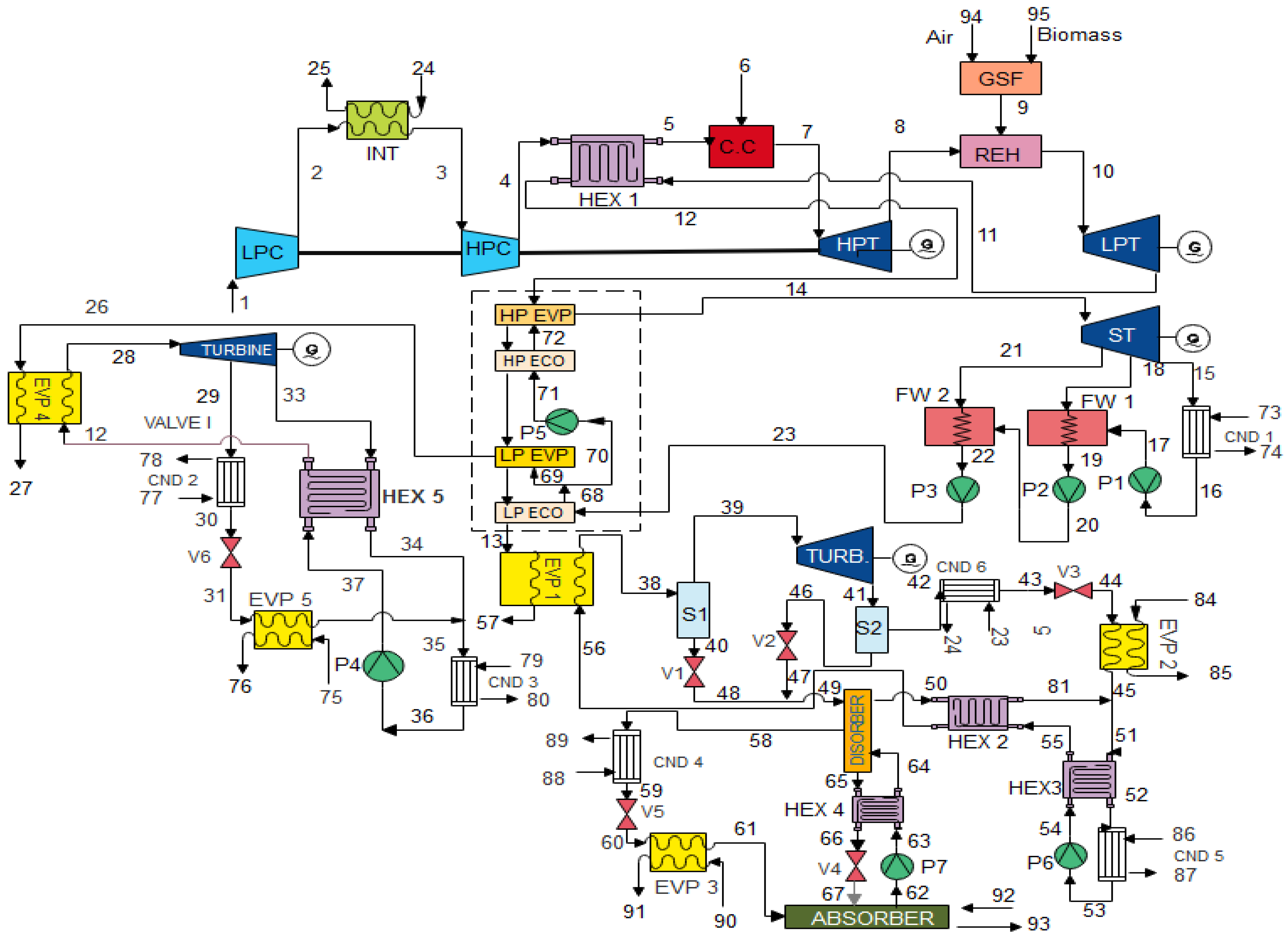
2.1. System Description

The proposed integrated multigeneration plant (IMP) is shown in Figure 1, which comprises five subsystems—a gas turbine (GT), steam turbine (ST), organic Rankine cycle (ORC) for cooling and power production, a modified Kalina cycle (KC) for power production and cooling, a vapor absorption system (VAB) for cooling, and a biomass syngas supplemental firing unit. From state 1, the air was drawn to the low-pressure compressor (LPC), raising the temperature and pressure of the air at state 2, which enters the intercooler (INT). The cooled air from the INT is recompressed by the high-pressure compressor (HPC), where it is combusted in the combustion chamber (C.C), after being partly heated by the expanded gas stream from the low-pressure turbine (LPT). The high-pressure turbine (HPT) drives both the HPC and LPC. The expanded gas from the HPT is reheated, by supplemental firing with the syngas from the biomass gasifier, which then expands in the LPT to produce shaft work. A portion of the expanded gas is recovered in a heat recovery steam generator (HRSG) to produce steam. The steam produced exists in two streams—the high-pressure steam, which drives the steam turbine (ST); and the low-pressure steam, which powers the vapor generator 1 (VG1 or EVP 1) for electrical energy production and cooling in an ORC power-cooling configuration. The superheated steam leaving the high-pressure evaporator (HP EVP) of the HRSG expands in the ST producing shaft work. Similarly, the steam is blended at two points, giving rise to two feedwater heaters (FW1 and FW2). Two feedwater heaters were introduced in order to optimally match the temperature at state 23, with the thermal energy demands of the other bottoming cycles. The heat obtained from the condensation of the expanded vapor is used for domestic hot water applications. The refrigerant in the vapor generator 2 (VG2 or EVP 4) in the ORC expands via the ORC turbine producing power. At the same time, part of the vapor is bled, throttled, condensed, and allowed to evaporate, thus providing cooling. The flue gas leaving the HRSG is used to power the KCPC integrated with a vapor absorption refrigeration system (VAB). Subsequently, the ammonia-water solution receives heat from the flue gas, leaving HRSG with the vapor expanding in the turbine, to produce electrical energy. The rich part of the mixture is further condensed and throttled and then allowed to evaporate in an evaporator, which provides a cooling effect. Similarly, the weak solution already expanded in the KC turbine mixes with the stream at state 47 (Figure 1), which heat the desorber for powering the VAB. The exiting stream at the desorber is passed through a heat exchanger before being added up, with the resulting stream beimg used for refrigeration at state 45. These stream summation produces the stream at state 51, which is pumped to the VG1 to commence the cycle. The proposed polygeneration system might look too complex, but it has strong potentials to provoke the development of the next generation polygeneration energy systems, beyond the academic environment. In addition, combine energy generation systems could and must be part of energy efficiency solutions, aimed at enhancing economic competitiveness, enhancing energy access, providing more affordable energy services, and reducing environmental impacts. The proposed system is very important to drive the current energy transition crisis caused by the COVID-19 pandemic shock wave in the energy sector [2].

2.2. Thermodynamic Modeling

In modeling the integrated multi-generation plant (IMP); Figure 1; analytical models were developed to describe the different subsystems that constitute the IMP: GT, ST, ORC, Gasifier, HRSG, KC, and VAB. The following assumptions were made [29,30,31]—(i) the system operates in a steady-state condition; (ii) the working fluid behaviors are considered ideal; (iii) the gasification reactions are in the equilibrium state; (iv) the potential energy and kinetic energy are neglected; and (v) the rich refrigerant is a strong solution, whereas the weak solution is rich in LiBr.H₂O.

The thermodynamic analysis is based on the following—first law of thermodynamics, the second law of thermodynamics, and the conservation of mass, as expressed in Equations (1)–(3), respectively [29,30,31].

$${{\displaystyle \sum }}_i{\dot{H}}_j-{{\displaystyle \sum }}_i{\dot{H}}_i=\dot{Q}-\dot{W}$$

(1)

$${\dot{E}}_{xD}={{\displaystyle \sum }}_i{\dot{E}}_{xi}-{{\displaystyle \sum }}_j{\dot{E}}_{xj}+{\displaystyle \sum }_k\left(1-\left(\frac{T_0}{T_k}\right)\right){\dot{Q}}_k-\dot{W}$$

(2)

$${{\displaystyle \sum }}_i{\dot{m}}_i={\displaystyle \sum }_j{\dot{m}}_j$$

(3)

2.2.1. ORC—Power Cooling System

The energy analysis in the vapor generator (ORCVG), rate of work transfer in the turbine (ORCT), capacity of the ORC evaporator (ORCEV), net power output of the ORC, thermal efficiency, exergy destruction rate in the ORC, and overall exergy efficiency of the ORC system are evaluated by the aid of Equations (4)–(10), respectively.

$${\dot{Q}}_{ORCVG}={\dot{m}}_g{c}_{pg}\left(h_{26}-h_{27}\right)-{\dot{m}}_{ref}\left(h_{28}-h_{37}\right)$$

(4)

$${\dot{W}}_{ORCT}={\dot{m}}_{ref}(h_{28}-h_{29})+\left({\dot{m}}_{ref}-{\dot{m}}_{refb}\right)\left(h_{29}-h_{33}\right)$$

(5)

$${\dot{Q}}_{ORCEV}={\dot{m}}_{ref}\left(h_{32}-h_{31}\right)$$

(6)

$${\dot{W}}_{ORC,net}={\dot{W}}_{ORCT}-{\dot{W}}_{ORCP}$$

(7)

$${\eta }_{th, ORC }=\frac{{\dot{W}}_{ORCT}+{\dot{Q}}_{ORCEV}}{{\dot{Q}}_{ORCVG}}\equiv \frac{{\dot{m}}_{ref}(h_{28}-h_{29})+\left({\dot{m}}_{ref}-{\dot{m}}_{refb}\right)\left(h_{29}-h_{33}\right)+{\dot{m}}_{ref}\left(h_{32}-h_{31}\right)}{{\dot{m}}_{gas}cpg\left(h_{26}-h_{27}\right)-{\dot{m}}_{ref}\left(h_{28}-h_{37}\right)}$$

(8)

$${\dot{E}}_{xD}ORC={\dot{E}}_{xD,ORCVG}+{\dot{E}}_{xD,ORCT}+{\dot{E}}_{xD,ORCC}+{\dot{E}}_{xD,ORCEV}+{\dot{E}}_{xD,ORCP}$$

(9)

$${\eta }_{ex,ORC}=\frac{{\dot{W}}_{ORCT+{\dot{E}}_{x}ORCEV}}{{\dot{E}}_{xin}}$$

(10)

2.2.2. Gas Turbine Plant (GT)

The work transfer rate in LPC and HPC, heat transfer rate in the CC, heat transfer rate in the REH (supplemental firing combustor), work transfer rate in the HPT and LPT, net power output and heat addition of the GT are determined from Equations (11)–(16), respectively.

$${\dot{W}}_{C,k}={\dot{m}}_k\left(h_i-h_j\right)$$

(11)

$${\dot{Q}}_{cc}={\eta }_{cc}{\dot{m}}_{fuel}{C}_v{}_{feul}$$

(12)

$${\dot{Q}}_{REH}={\eta }_{ccREH}{\dot{m}}_{biom}{C}_{v,biom}$$

(13)

$${\dot{W}}_{c,k}={\dot{m}}_k\left(h_i-h_j\right)={\dot{m}}_g{c}_{pg}\left(T_{\ddot{i}}-T_{\ddot{j}}\right)$$

(14)

where i, j and $\ddot{i}$,$\ddot{j}$ denote inlet and exit flow streams of the working fluid and flue gas, respectively; ${\dot{m}}_k$ is the mass flow rate for kth (where k = HPT and LPT)

$${\dot{W}}_{net}={\dot{W}}_{LPT}=\left(c{p}_{gas\left(T_{10}\right)}{T}_{10}-c{p}_{gas\left(T_{11}\right)}{T}_{11}\right)$$

(15)

$${\dot{Q}}_{in, total}={\dot{W}}_{LPT}=\left(c_p{}_{gas\left(T_7\right)}{T}_7-c_p{}_{gas\left(T_5\right)}\times T_5\right)+\left(c_p{}_{gas\left(T_{10}\right)}{T}_{10}-c_p{}_{gas\left(T_8\right)}{T}_8\right)$$

(16)

The thermal efficiency, ${\eta }_{th}$, exergy destruction rate,${\dot{E}}_{xD}$, and exergy efficiency, ${\eta }_{ex}$, in the GT are determined using Equations (17)–(19).

$${\eta }_{th,GT }=\frac{{\dot{W}}_{net}}{{\dot{Q}}_{in, total}}$$

(17)

$${\dot{E}}_{xD,GT}={\dot{E}}_{xD,LPC}+{\dot{E}}_{xD,INTC}+{\dot{E}}_{xD,HPC}+{\dot{E}}_{xD,CC}+{\dot{E}}_{xD,HPT}+{\dot{E}}_{xD,REH}+{\dot{E}}_{xD,LPT}$$

(18)

$${\eta }_{ex,GT}=1-\left(\frac{{\dot{E}}_{xD}GT}{{\dot{E}}_{x}GT,in}\right)$$

(19)

2.2.3. Kalina Cycle (KC)

The rate of heat transfer in the KC vapor generator (KCVG), the rate of work transfer in the KC turbine (KTUB), heat transfer in the KC evaporator (KEVP), rate of pump work in KC pump (KPUMP), thermal efficiency of the KC, rate of network of KC, exergy destruction rate, and exergetic efficiency of the KC are computed, respectively, by Equations (20)–(27):

$${\dot{Q}}_{KVG}={\dot{m}}_{13}{h}_{13}-{\dot{m}}_{57}{h}_{57}={\dot{m}}_{38}{h}_{38}-{\dot{m}}_{56}{h}_{56}$$

(20)

$${\dot{W}}_{KTUB}={\dot{m}}_3{h}_3-{\dot{m}}_4{h}_4$$

(21)

$${\dot{W}}_{KPUM}={\dot{m}}_{54}{h}_{54}-{\dot{m}}_{53}{h}_{53}$$

(22)

$${\dot{W}}_{KPUM}={\dot{m}}_{54}{h}_{54}-{\dot{m}}_{53}{h}_{53}$$

(23)

$${\eta }_{th, KPCC}=\frac{{\dot{W}}_{net}+{\dot{Q}}_{evap,KC}}{{\dot{Q}}_{in}, KC}$$

(24)

$${\dot{W}}_{net, kc}={\dot{W}}_{KTUB}-{\dot{W}}_{KPUM}$$

(25)

$${\dot{E}}_{xD,KC}={\dot{E}}_{xD,KVG}+{\dot{E}}_{xD,KTUB}+{\dot{E}}_{xD,EVP}+{\dot{E}}_{xD,KCON}+{\dot{E}}_{xD,KPUM}+{\displaystyle \sum }_k{\dot{E}}_{xD,KHEX}+{\displaystyle \sum }_k{\dot{E}}_{xD,KSP}$$

(26)

$${\eta }_{ex}=\frac{{\dot{W}}_{net,KC}+{\dot{E}}_{evap,KC}}{{\dot{Ex}}_{in}, total}$$

(27)

2.2.4. Vapor Absorption System (VAB)

The heat transfer rate in the VAB desorber (VABD), heat transfer rate in the VAB condenser, heat transfer rate in VAB evaporator (VABEV), heat transfer rate in the VAB absorber (VABAB), rate of pump work of the VAB (VABP), and coefficient of performance of the VAB are expressed, respectively, by Equations (28)–(33), thus

$${\dot{Q}}_{VABD}={\dot{m}}_{49}{h}_{49}+{\dot{m}}_{64}{h}_{64}={\dot{m}}_{50}{h}_{50}+{\dot{m}}_{58}{h}_{58}+{\dot{m}}_{65}{h}_{65}$$

(28)

$${\dot{Q}}_{VABC}={\dot{m}}_{58}{h}_{58}-{\dot{m}}_{59}{h}_{59}$$

(29)

$${\dot{Q}}_{VABE}={\dot{m}}_{61}{h}_{61}-{\dot{m}}_{60}{h}_{60}$$

(30)

$${\dot{Q}}_{VABA}={\dot{m}}_{61}{h}_{61}+{\dot{m}}_{67}{h}_{67}-{\dot{m}}_{62}{h}_{62}$$

(31)

$${\dot{W}}_{VABP}={\dot{m}}_{63}{h}_{63}-{\dot{m}}_{62}{h}_{62}$$

(32)

$$COP=\frac{{\dot{Q}}_{VABE}}{{\dot{W}}_{VABP}+{\dot{Q}}_{VABD}}$$

(33)

The mass flow rates of the working fluid, strong (${\dot{m}}_{ss}$) and a weak solution (${\dot{m}}_{ws}$) could be computed, respectively, by Equations (34) and (35)

$${\dot{m}}_{ws}=\frac{{\xi }_{ss}}{{\xi }_{ws}+{\xi }_{ss}}$$

(34)

$${\dot{m}}_{ss}=\frac{{\xi }_{ws}}{{\xi }_{ws}+{\xi }_{ss}}$$

(35)

where ${\xi }_{ss}$ and ${\xi }_{ws}$ are defined by [32]

$${\xi }_{ss}=\frac{49.04+1.125t_a-t_e}{134.65+0.47t_a}$$

(36)

$${\xi }_{ws}=\frac{49.04+1.125t_g-t_c}{134.65+0.47t_g}$$

(37)

where ${\xi }_{ws}$ and ${\xi }_{ss}$ are weak and strong solutions of LiBr.H₂O (lithium-bromide) concentration of the refrigerant in that order; $t_a$, $t_e$, $t_c$, and $t_g$ are temperatures of absorber, evaporator, condenser, and desorber, respectively. Specifics of the correlations of entropy and enthalpy and LiBr-H₂O are presented elsewhere [32].

2.2.5. Steam Turbine Cycle (STC)

The heat transfer rate across the HP evaporator, HP economizer, LP evaporator, LP economizer and HRSG could be calculated by Equation (38).

$${\dot{Q}}_k={\dot{m}}_k\left(h_i-h_j\right)={\dot{m}}_{gas}{c}_{pgas}\left(T_i-T_j\right)$$

(38)

The work transfer rate in LP and HP steam turbines could be computed by Equation (39), thus,

$${\dot{W}}_{st,k}={\dot{m}}_k\left(h_i-h_j\right)$$

(39)

The heat rejection rate in the steam turbine condenser (SC) is computed as follows:

$${\dot{Q}}_{SC}={\dot{m}}_w\left(h_i-h_j\right)$$

(40)

Equation (41) can be used to compute the power of HP and LP water feed pump

$${\dot{W}}_{fwp,k}={\dot{m}}_k\left(h_i-h_j\right)$$

(41)

The net power output of the ST cycle is estimated by Equation (42)

$${\dot{W}}_{STC}={\displaystyle \sum }_k{\dot{W}}_{st, k}-{\displaystyle \sum }_k{\dot{W}}_{fwp, k}$$

(42)

The exergy destruction rate in the ST is calculated by Equation (43)

$${\dot{E}}_{xD,STC}={\displaystyle \sum }_k{\dot{E}}_{xD,HRSG}+{\displaystyle \sum }_k{\dot{E}}_{xD,ST}+{\displaystyle \sum }_k{\dot{E}}_{xD,SC}+{\displaystyle \sum }_k{\dot{E}}_{xD,FWP}$$

(43)

The thermal efficiency (${\eta }_{th}$) and the exergy efficiency (${\eta }_{ex}$) are computed by Equations (44) and (45), respectively.

$${\eta }_{th,STC }=\frac{{\dot{W}}_{STC,net}}{{{\displaystyle \sum }}_k{\dot{Q}}_k}$$

(44)

$${\eta }_{ex,STC}=1-\left(\frac{{\dot{E}}_{xD}STC}{{\dot{E}}_{x}STC,in}\right)$$

(45)

2.2.6. Gasifier Model

The global gasification reaction for biomass (wood) considered in this study is expressed in [18,19].

$$C_n{H}_x{O}_y{N}_x+m\left(O_2+3.76N_2\right)\to {\overline{n}}_{H_2}{H}_2+{\overline{n}}_{CO}CO+{\overline{n}}_{C{O}_2}+{\overline{n}}_{H_{2}O}{H}_{2}O+{\overline{n}}_{C{H}_4}C{H}_4+\left(\frac{z}{2}+3.76m\right)N_2$$

(46)

where $C_n{H}_x{O}_y{N}_x$ is the chemical formulation, ${\overline{n}}_i$ denotes molar composition for the $i\mathrm{th}$element of the syngas, which is estimated from atomic, equilibrium reactions [19,33]. Similarly, the energy balance in the gasifier is described by Equation (47).

$$\begin{gathered} h_f^0{}_{biomas}+m\left(h_f^0{}_{O_2}+3.76h_f^0{}_{N_2}\right)={\displaystyle \sum }{\overline{n}}_i{h}_f^0+\left[\left({{\displaystyle \sum }}_i{\overline{n}}_i{c}_{1i}\right)T+\left({{\displaystyle \sum }}_i{\overline{n}}_i{c}_{2i}\right)T^2+ \\ \left({{\displaystyle \sum }}_i{\overline{n}}_i{c}_{3i}\right)T^3+\left({{\displaystyle \sum }}_i{\overline{n}}_i{c}_{4i}\right)T^4+\left({{\displaystyle \sum }}_i{\overline{n}}_i{k}_i\right)\right] \end{gathered}$$

(47)

where $h_f^0{}_{biomas}$, $h_f^0{}_{O_2}$, and $h_f^0{}_{N_2}$ are enthalpy of formations for biomass, oxygen, and nitrogen gas, respectively; $m$ denotes the number of moles of air, $T$ is the temperature of the product, and $c_{ij}$ represents the heat constant (specific) for all the syngas species.

2.2.7. The Integrated Multi-Generation Plant (IMP)

The overall energy efficiency and exergy efficiency of the IMP are expressed as follow:

$${\eta }_{th, IMP}= \frac{Outpu{t}_{total}}{{\dot{Q}}_{in,total}}$$

(48)

$${\eta }_{ex, IMP}=\frac{{\dot{Ex}}_{out}{,}_{total}}{{\dot{Ex}}_{in, total}}$$

(49)

where

$$Outpu{t}_{total}= {\dot{W}}_{LPT}+{\dot{W}}_{HPT}+{\dot{W}}_{ST}+{\dot{W}}_{GT}+{\dot{W}}_{ORCT}+{\dot{Q}}_{col,}{}_{KC}+{\dot{Q}}_{col,}{}_{VAS}+{\dot{Q}}_{col,}{}_{ORC}$$

(50)

2.3. Environmental Modeling

The environmental impact is determined by computing the quantity of the pollutants produced according to the empirical relations presented in [19,34], which include nitrogen oxide, ${\dot{m}}_{NOx}$ (kg/s), carbon dioxide, ${\dot{m}}_{C{O}_2}$ (kg/s), and carbon mono oxide, ${\dot{m}}_{CO}$ (kg/s). The amount of these harmful emissions produced and their rates is a function of the following parameters—retention time, τ (s), adiabatic flame temperature, $T_{pz}$, combustion chamber pressure drop, $∆PCC$ (kPa), as presented in [19,34]. Therefore, the emission rates and the harmful fuel emission factor, $F_{EF}$, are defined in Equations (51)–(55), which are well established and proven empirical relations.

$${\dot{m}}_{N{O}_x}=\frac{1.5\times {10}^{15}{\tau }^{0.5}{e}^{-\left(7110/T_{pz}\right)}}{P_6{}^{0.05}{\left(\frac{\mathsf{\Delta }PCC}{P_6}\right)}^{0.5}}$$

(51)

$${\dot{m}}_{CO}=\frac{1.79\times {10}^8{\tau }^{0.5}{e}^{\left(7800/T_{pz}\right)}}{P_6{}^{0.05}\tau {\left(\frac{\mathsf{\Delta }PCC}{P_6}\right)}^{0.5}}$$

(52)

$${\dot{m}}_{C{O}_2}=yC{O}_2{\dot{m}}_g\left(\frac{{\overline{M}}_{C{O}_2}}{{\dot{m}}_g}\right)$$

(53)

$$c{o}_{2, sp}=3600\left(\frac{{\dot{m}}_{C{O}_2}}{{\dot{W}}_{net}}\right)$$

(54)

$$F_{EF}=\frac{{\dot{M}}_{N{O}_x}+{\dot{M}}_{CO}+{\dot{M}}_{C{O}_2}}{{\dot{m}}_g}$$

(55)

where $C{O}_{2,sp}\left(k{g}_{C{O}_2/MWh}\right)$ depicts the quantity and specific $C{O}_2$ emissions, respectively. Equally, ${\dot{m}}_g$, $\overline{M}$, $yC{O}_2$ and ${\overline{M}}_{C{O}_2}$ are mass flow rate of flue gas, molar mass of flue gas, mass fraction, and the molar mass of $C{O}_2$. The adiabatic flame temperature $T_{pz}$ could be defined by Equation (56). All parameters, constants and the terms x, y, and z in Equation (57) were estimated according to the procedure presented in [34,35].

$$T_{pz}=A{\sigma }^{\alpha }\exp \left[\beta {\left(\sigma +\lambda \right)}^2\right]{\pi }^{x^{\ast }}{\theta }^{y^{\ast }}{\psi }^{z^{\ast }}$$

(56)

2.4. Sustainability Modeling

The sustainability index (SI) is an index that described the capacity and effective utilization and preservation of the energy resources [36]. The SI was evaluated using Equation (57).

$$SI=\frac{1}{1-{\eta }_{ex}}$$

(57)

Furthermore, novel ideas considered for sustainability estimation in this study comprise exergetic utility exponent (EUE) and exergo-thermal index (ETI). The EUE defines the degree at which exergy of the resource input is used for work production according to Equation (58). The small values of EUE presage poor process conversion, especially for multi-generation systems. For constant ${\dot{E}}_{xin}$, the value of EUE increases as ${\dot{E}}_{xout }\to 0$, and the $\mathit{EUE}$approaches the system exergy efficiency. The implication is that EUE is bounded by $0<EUE<1$.

$$EUE= \frac{{\eta }_{CC}{\dot{W}}_{net}}{{\dot{E}}_{xin}-{\dot{E}}_{xout}}$$

(58)

where ${\eta }_{CC}$, ${\dot{W}}_{net}$, ${\dot{E}}_{xin}$, and ${\dot{E}}_{xout}$ are the combustion chamber efficiency, total work output, exergy input from the fuel, and exergy output from the exhaust stream. Similarly, the ETI quantifies the thermal impact of the energy generation system on the environment, subject to a physical environment, as defined in Equation (59). The ETI increases with an increase in $T_{exhuast}$; the low values of ETI are desired and connote less environmental impact.

$$ETI= \frac{EUE}{\Im } = \frac{{\eta }_{CC}{\dot{W}}_{net}}{\left({\dot{E}}_{xin}-{\dot{E}}_{xout}\right)}\times \frac{1}{\Im }\equiv \frac{{\eta }_{CC}{\dot{W}}_{net}{T}_{ext}}{T_{ev}\left({\dot{E}}_{xin}-{\dot{E}}_{xout}\right)}$$

(59)

where $\Im$, the thermal pollution factor, represents the ratio of the environmental temperature ($T_{ev}$) to that of the exhaust stream ($T_{exh}$), according to Equation (60).

$$\Im =\left(T_{ev}/T_{exh}\right)$$

(60)

2.5. Economic Analysis

The exergoeconomic assessment was performed to determine the competitiveness of the proposed plant with the existing power plants, and also, to suggest the system components that need to be redesigned to reduce the exergy destruction rate. The SPecific Exergy Cost (SPECO) method was applied in the current analysis. The SPECO method is derived from exergy, system cost for product and resource utilization per unit of exergy, coupled with closure equations [37]. The equations defining the component cost of the IMP are presented in

Table 1. Equipment cost [19,38,39].

Components	$\mathbf{Cost} \mathbf{Function} {\mathit{Z}}_{\mathit{k}}\left(\mathit{\$}\right)$
Gasifier	$2.9\times {10}^6{\left(3.6\dot{m}\right)}^{0.7}$
Air compressor	$\frac{39.5\dot{ma}}{0.9-{\eta }_C}\left(\frac{P_i}{P_j}\right)ln\left(\frac{P_i}{P_j}\right)$
GT	${\dot{W}}_{GT}1318.5-98.328ln\left({\dot{W}}_{GT}\right)$
HRSG	$4745{\left(\frac{\dot{QHRGS}}{log\left(∆THRSG\right)}\right)}^{0.7}+1182{\dot{m}}_g$
Steam turbine	$600{\left({\dot{W}}_{ST}\right)}^{0.7}$
Steam condenser	${\dot{17773m}}_w$
Feedwater pump	$3540{\left({\dot{W}}_{FWP}\right)}^{0.71}$
ORC evaporator	$309.14{\left(\frac{{\dot{Q}}_{HRVG}}{0.2∆T_{HRVG}}\right)}^{0.85}$
ORC-turbine	$4750{\left({\dot{W}}_{ORCT}\right)}^{0.75}$
ORC-condenser	$516.62\left(\frac{{\dot{Q}}_{ORCC}}{0.15∆T_{ORCC}}\right)$
ORC-pump	$705.5{\left(0.001{\dot{W}}_{ORCP}\right)}^{0.71}\left(1+\frac{0.2}{{\eta }_P}\right)$
VAB-condenser	${\dot{17773m}}_w$
VAB-evaporation	$130{\left(\frac{A_{VABE}}{0.093}\right)}^{0.78}$
VAB-absorber	$130{\left(\frac{A_{VABA}}{0.093}\right)}^{0.78}$
VAB-throttle valve	$37{\left(\frac{P_i}{P_j}\right)}^{0.68}$
VAB solution pump	$800{\left(\frac{{\dot{W}}_{VABP}}{100}\right)}^{0.26}{\left(\frac{1-{\eta }_{SP}}{{\eta }_{SP}}\right)}^{0.5}$

. The cost relations ranged between the years 2008 and 2016. The range might not cover the present reality of the cost estimate. Nonetheless, they could well be considered an initial approximation for this assessment, without much deviation in the accuracy of the results. The general exergoeconomic balance for an exergy conversion system was related as follows:

$$c_{q,k}{\dot{E}}_{q,k }+ {{\displaystyle \sum }}_i{\left(c_i\dot{E_i}\right)}_k +{\dot{Z}}_k = {{\displaystyle \sum }}_e{\left(c_e\dot{E_e}\right)}_k +c_{w,k}{\dot{W}}_k$$

(61)

where ${{\displaystyle \sum }}_e{\left(c_e\dot{E_e}\right)}_k$ is cost rates associated with exit exergy streams of the $k\mathrm{th}$component; $c_{w,k}{\dot{W}}_k$ is the cost rates of power generation of the $k\mathrm{th}$ component; $c_{q,k}{\dot{E}}_{q,k}$ is the cost rates associated with heat transfer of the $k\mathrm{th}$ component; ${{\displaystyle \sum }}_i{\left(c_i\dot{E_i}\right)}_k$is the cost rates associated with entering exergy streams of the $k\mathrm{th}$ component; ${\dot{Z}}_k$ is the capital investment cost rate of the $k\mathrm{t}\mathrm{h}$ component, and $c$ connote specific cost.

The average exergoeconomic cost parameters, namely unit cost of fuel, $c_{F,k}$, unit cost of product, $c_{P,k}$, and cost rate of exergy destruction, $C_{D,k}$, are defined in Equations (62)–(64), respectively; whereas the exergoeconomic factor, $f_k$, and relative cost difference, $r_k$, for the k^th component are defined by Equations (65) and (66) [38].

$$c_{F,k}=\frac{{\dot{C}}_{F,k}}{{\dot{E}}_{F,k}}$$

(62)

$$c_{P,k}=\frac{{\dot{C}}_{P,k}}{{\dot{E}}_{P,k}}$$

(63)

$$c_{D,k}=c_{F,k}{\dot{E}}_{D,k}$$

(64)

$$f_k = \frac{{\dot{z}}_k}{{\dot{z}}_k+{\dot{c}}_{D,k}+{\dot{z}}_{D,k}}$$

(65)

$$r_k=\frac{C_{P,k}-C_{F,k}}{C_{F,k}}$$

(66)

The exergoeconomic factor and the relative cost difference are important parameters in the prioritization of the system’s components for improvement. The exergoeconomic factor weighs the investment cost against irreversibility caused by a specific system’s component, whereas the relative cost difference weighs relative increase in cost per exergy, against the unit cost of fuel input.

The sum of the total capital investment, ${\dot{Z}}_k^{CI}$, and operation and maintenance cost,${\dot{Z}}_k^{OM}$, constitutes the overall cost rate of the kth component (${\dot{z}}_k$), as presented in Equation (67) [39].

$${\dot{Z}}_k = {\dot{Z}}_k^{CI} + {\dot{Z}}_k^{OM}$$

(67)

The annual levelized capital investment for the kth component is evaluated according to [39]:

$${\dot{Z}}_k=CRF\frac{{\varnothing }_k}{N\times 3600}{Z}_k$$

(68)

where $Z_k$, N, ${\varphi }_k$, and $CRF$ represent the cost of purchasing the $k$th equipment, the yearly number of operating hours of the component functions, the maintenance factor, and CRF, represents the capital recovery factor, respectively. The capital recovery factor could be estimated by Equation (69).

$$CRF=\frac{i{\left(1+i\right)}^n}{{\left(1+i\right)}^n-1}$$

(69)

where i and n represent the interest rate and the expected operational life of the system. The values of 0.15 and 20 years were adopted for the interest rate and the system operational life, according to [39].

The economic figures of merit of the proposed IMP and other economic parameters are presented according to [40]. Therefore, the unit cost of electricity, UCE ($/kWh), could be estimated by Equation (70).

$$UCE=\frac{Z_{ALCC}}{365\times E_{DP}}$$

(70)

where $E_{DP}$ is the daily energy produced by IMP $\left(24\times {\dot{W}}_{net}\right)$ and the $Z_{ALCC}$ is defined by [38].

$$Z_{ALCC}=CRF{Z}_{LCC}$$

(71)

$$\begin{array}{l}\mathrm{LCC}={\displaystyle {\displaystyle \sum }_q^Z}{C}_q;q ϵ\left(1,2,\dots \right)\\ \equiv \left(\mathrm{VG}, \mathrm{TURB}, \mathrm{HRSG} \mathrm{GASF}, \mathrm{EVAP},\mathrm{PUMP}, \mathrm{COND}, \mathrm{HEX}, \mathrm{ABS}, \mathrm{DES}\right)\end{array}$$

(72)

where Cq ($) represents the plant components cost, q

The break-even point (BEP) or payback time (PBT) is determined with the aid of Equation (73), as expressed in [40]

$$BEP=\frac{LCC}{C_{Tarrif}{A}_{EP}}$$

(73)

where $Z_{LCC}$, $Z_{ALCC}$($), $Z_i$ ($), $C_{Tarrif}$ ($/kWh), $A_{EP}$ (kWh/y) are the life cycle cost, the selling price per unit of electricity, and yearly energy production, respectively.

3. Results and Discussion

All the equations were programmed in the Engineering Equation Solver software platform to facilitate the ease of computation and simulation of the system.

3.1. Thermodynamic Performance of the IMP

The input parameters used for thermodynamic modeling are shown in

Table 2. Thermodynamic input parameters and simulation data for the proposed integrated multi-generation plant (IMP) [13,15,16,19,25,31,32,33,34,35,36,37,38,39,40,41,42,43].

Parameter	Symbol	Unit	Value
Ambient temperature	$T_0$	°C	25
Ambient Pressure	$P_0$	bar	1.013
GT Lower compression ratio	$P_2/P_1$	-	3.162
GT Higher compression ratio	$P_4/P_3$	-	3.162
Overall pressure ratio	$P_4/P_1$	-	10
GT Heat exchanger effectiveness	$\epsilon$	%	75
Low-pressure turbine isentropic efficiency	${\eta }_{LPT}$	%	85
High-pressure turbine isentropic efficiency	${\eta }_{HPT}$	%	85
Low-pressure compressor isentropic efficiency	${\eta }_{LPC}$	%	80
High-pressure compressor isentropic efficiency	${\eta }_{HPC}$	%	80
mass of air to the topping cycle	$m_{air}$	kg/s	418
mass of gas at the inlet to the first combustion chamber	$m_6$	kg/s	3.131
mass of gas at the inlet to the supplemental firing combustor (reheater)	$m_9$	kg/s	21.49
The high-pressure turbine inlet temperature	$T_7$	°K	1350
The low-pressure turbine inlet temperature	$T_{10}$	°K	1200
The exit temperature of intercooler water	$T_{25}$	°C	85
pinch point temperature for HP evaporator	$P{P}_{HPE}$	°C	25
pinch point temperature for LP evaporator	$P{P}_{LPE}$	°C	25
HRSG higher pressure	$P_{72}$	bar	25
HRSG lower pressure	$P_{68}$	bar	10
Steam turbine isentropic efficiency	${\eta }_{ST}$	%	85
ST inlet pressure	$P_{14}$	bar	25
ST inlet temperature	$T_{14}$	°C	350
ST bled pressure	$P_{21}$	bar	0.05
ST condenser pressure	P15	bar	0.08
ORC turbine inlet temperature	$T_{28}$	°C	90
ORC turbine inlet pressure	$P_{28}$	bar	16.7
ORC turbine back pressure	$P_{33}$	bar	6.87
ORC evaporator temperature	$T_{31}$	°C	−2
Kalina turbine inlet temperature	$T_{39}$	°C	180
Kalina turbine inlet pressure	$P_{39}$	bar	20
Kalina turbine back pressure	$P_{41}$	bar	7
Kalina evaporator temperature	$T_{44}$	°C	−5.49
VAS evaporator temperature	$T_{60}$	°C	1.651
HRSG lower pressure	$P_{68}$	bar	10

. The outcomes of the thermodynamic and environmental performance of the IMP are depicted in

Table 3. Thermodynamic performance of the IMP.

Unit	Parameters	Units	Value
Gas turbine	Net power	MW	148.73
	Thermal efficiency	%	35.91
	Exergy efficiency	%	35.79
Steam turbine	Net power	MW	35.08
	Thermal efficiency	%	32.52
	Exergy efficiency	%	35.15
ORC-power cooling	Net power	MW	42.82
	Thermal efficiency	%	18.81
	Exergy efficiency	%	22.22
	Cooling load	kW	45.36
Kalina-power cooling	Net power	kW	36.27
	Thermal efficiency	%	16.96
	Exergy efficiency	%	20.43
	Cooling load	kW	36.27
Vapor absorption	Exergy of cooling	kW	11.12
	COP	-	0.472
	Cooling load	kW	130.5
	Desorber heat	kW	162.1
Integrated multigeneration plant (IMP)	Net power	MW	183.91
	Thermal efficiency	%	61.5
	Exergy efficiency	%	44.22

and

Table 4. Environmental and sustainability parameters.

Parameters	Symbol	Units	Value
${\mathrm{NO}}_{\mathrm{z}}$ emission rates	${\dot{m}}_{N{O}_x}$	kg/s	0.222
$\mathrm{CO}$ emission	$\dot{m}CO$	kg/s	3.0 × 10−7
Specific ${\mathrm{CO}}_2$ emission	$C{O}_{2,spe}$	${\mathrm{kg}}_{{\mathrm{CO}}_2/\mathrm{MWh}}$	122.2
Fuel emission harmful factor	$F_{EF}$	-	0.00066
Exergetic utility exponent	EUI	-	0.7335
Exergo-thermal index	ETI	-	0.675
Sustainability index	SI	-	1.434

, respectively. The parameters of the state points of the proposed system are presented in

Table A1. Thermodynamic state point properties for the gas turbine in the IMP.

State	T (°C)	P (bar)	h (kJ·kg−1)	s (kJ·kg·K−1)	m (kgs−1)	$\dot{\mathit{e} }\left({\mathbf{kJ·kg}}^{-1}\right)$	$\dot{\mathit{E}} (\mathbf{kJ}/\mathbf{s})$
1	25.0	1.013	299.4	5.695	200.00	0.00	0.000
2	170.1	3.203	451.6	5.765	200.00	131.40	26,280.0
3	120.0	3.203	397.9	5.643	200.00	113.90	22,774.0
4	311.3	10.13	611.9	5.72	200.00	305.20	61,034.0
5	583.0	10.13	951.1	6.131	200.00	521.80	104,359.0
6	25.0	10.13	43,852.0	-	3.131	49,349.00	15,4511
7	1077.0	10.13	1612.0	6.656	203.1	1027.00	20,8504
8	815.0	3.203	1259.0	6.734	203.1	649.90	131,993
9	627.0	3.203	2832.0	-	21.49	2064.00	44,347
10	927.0	3.203	1409.0	6.848	224.6	766.40	172,140
11	673.5	1.013	1070.0	6.905	224.6	410.10	92,106
12	401.9	1.013	721.2	6.533	224.6	172.10	38,653
24	20.0	1.013	83.3	0.294	42.84	0.00	0.000
25	80.0	1.013	334.3	1.073	42.84	18.77	803.9

,

Table A2. Thermodynamic state points properties for the steam turbine in the IMP.

State	T (°C)	P (bar)	h ((kJ·kg−1)	s (kJ·kg·K−1)	m (kgs−1)	$\dot{\mathit{e} }\left({\mathbf{kJ·kg}}^{-1}\right)$	$\dot{\mathit{E}} (\mathbf{kJ}/\mathbf{s})$
14	350.00	25.00	3125.0	6.839	19.22	1091.00	20,978
15	41.60	0.08	2139.0	6.839	14.59	105.60	1540
16	41.60	0.08	173.7	0.592	14.59	1.602	23.38
17	41.60	1.50	173.9	0.592	14.59	1.75	25.47
18	111.50	1.50	2546.0	6.839	3.176	511.60	1625
19	111.50	1.50	467.1	1.433	17.76	44.22	785.4
20	111.50	5.00	467.4	1.433	17.76	44.59	792.0
21	155.30	5.00	2756.0	6.839	1.451	722.30	1048
22	152.00	5.00	640.3	1.861	19.22	90.06	1731
23	152.10	10.00	640.8	1.861	19.22	90.63	1742
68	165.00	10.00	697.2	1.988	19.72	106.40	2098
69	165.00	10.00	697.2	1.988	0.50	4196.00	2098
70	165.00	10.00	697.2	1.988	19.22	109.20	2098
71	165.20	25.00	698.8	1.991	19.22	109.70	2108
72	209.1	25	893.2	2.414	19.22	178.10	3424

,

Table A3. Thermodynamic state point properties for the Kalina cycle in the IMP.

State	T (°C)	P (bar)	h (kJ·kg−1)	s (kJ·kg·K−1)	m (kgs−1)	$\dot{\mathit{e} }\left({\mathbf{kJ·kg}}^{-1}\right)$	$\dot{\mathit{E}} (\mathbf{kJ}/\mathbf{s})$
13	201.10	1.013	485.8	-	224.600	46.45	10,433
39	180.00	20.00	2164.0	5.901	0.193	625.6	121.00
40	180.00	20.00	694.1	2.205	0.305	135.1	41.22
41	136.90	7.00	1971.0	5.901	0.193	432.6	83.67
42	136.90	7.00	2080.0	6.209	0.181	455.8	82.31
43	42.90	7.00	−42.60	0.480	0.181	40.75	7.36
44	−5.50	0.80	−42.60	0.5609	0.181	16.66	3.01
45	15.00	0.80	332.40	1.909	0.181	−10.18	−1.84
46	136.90	7.00	509.50	1.753	0.013	72.78	0.95
47	77.60	0.80	509.50	1.821	0.013	52.57	0.68
48	79.80	0.80	694.10	2.390	0.305	79.84	24.36
49	79.70	0.80	686.70	2.367	0.318	78.74	25.04
56	50.00	20.00	35.55	0.6514	0.499	6.364	3.17
57	150.00	1.013	437.30	6.048	12.630	32.59	411.60
82	20.00	1.013	83.30	0.294	4.581	0.00	0.00
83	40.00	1.013	167.00	0.5702	4.581	1.351	6.19

,

Table A4. Thermodynamic state point properties for the vapor absorption cycle in the IMP.

State	T (°C)	P (bar)	h (kJ·kg−1)	s (kJ·kg·K−1)	m (kgs−1)	$\dot{\mathit{e} }\left({\mathbf{kJ·kg}}^{-1}\right)$	$\dot{\mathit{E} }(\mathbf{kJ}/\mathbf{s})$
50	60.0	0.800	176.8	0.8905	0.3180	8.989	2.858
51	43.3	0.800	213.8	1.2360	0.4986	10.310	5.142
52	38.0	0.800	123.0	0.9479	0.4986	5.441	2.713
53	25.0	0.800	−73.38	0.3073	0.4986	−0.024	−0.012
54	25.1	20.000	−71.24	0.3073	0.4986	2.110	1.052
55	40.0	20.000	−7.271	0.5168	0.4986	3.674	1.832
58	74.7	0.074	2639.0	8.4510	0.4986	14.020	6.988
59	41.0	0.074	171.1	0.5836	0.0560	1.463	0.082
60	1.7	0.007	171.1	0.6229	0.0560	−10.230	−0.573
61	1.7	0.007	2503.0	9.1140	0.0560	−208.500	−11.670
62	34.6	0.007	92.0	0.1987	0.4164	0.271	0.113
63	34.6	0.074	92.0	0.1987	0.4164	0.275	0.114
64	67.0	0.074	156.3	0.3978	0.4164	5.259	2.190
65	74.7	0.074	220.6	0.3917	0.3605	2.915	1.051
66	45.0	0.074	169.3	0.2361	0.3605	−1.975	−0.712
67	35.0	0.007	169.3	0.1817	0.3605	14.220	5.128
86	20.0	1.013	83.3	0.2940	1.1700	0.000	0.000
87	32.0	1.013	167.0	0.5702	1.1700	1.350	1.580
88	20.0	1.013	83.3	0.294	1.6510	0.000	0.000
89	40.0	1.013	167.0	0.5702	1.6510	1.351	2.230
90	25.0	1.013	299.4	5.6950	5.8400	3.009 × 10−36	0.000
91	3.0	1.013	277.0	5.618	5.8400	0.599	3.496
92	20.0	1.013	83.3	0.2940	2.5950	0.000	0.000
93	35.0	1.013	146.0	0.5029	2.5950	0.509	1.321

and

Table A5. Thermodynamic state points properties for the organic Rankine cycle in the IMP.

State	T (°C)	P (bar)	h ((kJ·kg−1)	s (kJ·kg·K−1)	m (kgs−1)	$\dot{\mathit{e} }\left({\mathbf{kJ·kg}}^{-1}\right)$	$\dot{\mathit{E} }(\mathbf{kJ}/\mathbf{s})$
26	180.0	10.00	1147.0	2.986	0.500	261.20	130.60
27	50.0	10.00	209.6	0.701	0.500	4.88	2.44
28	90.0	16.70	436.6	1.727	2.722	59.66	162.40
29	80.9	12.90	431.2	1.727	0.463	54.26	25.11
30	45.0	12.90	263.9	1.214	0.463	39.82	18.43
31	−2.0	6.87	263.9	1.236	0.463	33.17	15.35
32	−2.0	6.87	362	1.598	0.463	23.40	10.83
33	61.0	6.87	417.7	1.727	2.259	40.73	92.01
34	27.3	6.87	382.2	1.615	2.259	38.62	87.25
35	25.0	6.87	234.1	1.118	2.722	12.81	34.87
35′	25.6	16.70	378.8	1.603	2.722	38.61	105.10
36	25.6	16.70	235.0	1.121	2.722	38.43	104.60
37	45.0	16.70	264.5	1.214	2.722	40.34	109.80
75	25.0	1.013	299.4	5.695	1.942	0.00	0.00
76	2.0	1.013	276.0	5.614	1.942	0.67	1.30
77	20.0	1.013	83.3	0.294	0.925	0.00	0.00
78	40.0	1.013	167.0	0.570	0.925	1.35	1.25
79	20.0	1.013	83.3	0.294	3.766	0.00	0.00
80	45.0	1.013	187.9	0.637	3.766	2.51	9.45

in the Appendix A. Further results are displayed in graphical plots to show the simulated results.

From Table 3, the thermal efficiency (energy efficiency) for the system units varies from 16.96 to 35.91%, while the exergy efficiency ranges between 20.43 and 35.15%. The energy and exergy efficiencies of the IMP stood at 61.5 and 44.22%, respectively, with a net power output of 183.91 MW.

From Table 4, the harmful fuel emission factor, $F_{EF}$, and the exergetic utility exponent, EUE, were estimated at 0.00066 and 0.7335, respectively, which are indicative of better plant performance. The specific CO₂ emission was estimated at $122.1{ \mathrm{kgCO}}_2/\mathrm{MWh}$, see Table 4. The specific CO₂ emission obtained from this study was improved when compared to the $408.78{ \mathrm{kgCO}}_2/\mathrm{MWh}$ and $518.80{ \mathrm{kgCO}}_2/\mathrm{MWh}$ values obtained from the studies of [35] and [42]. The discrepancies in these results are ascribed to plant capacity, plant configuration, and type of fuel. Furthermore, ETI and SI were estimated at 0.675 and 1.43 for the IMP in that order.

3.1.1. Validation and Comparison of Results

The IMP performance was validated and compared with results of biomass integrated multigeneration energy systems in the open domain, as shown in

Table 5. Results validation with IMP.

S/N	Study	Reference	Energy Efficiency, %	Exergy Efficiency, %
1	Development and techno-economic assessment of a new biomass-assisted integrated plant for multi-generation	[44]	63.62	59.26
2	Development and analysis of a novel biomass-based integrated system for multi-generation with hydrogen production	[45]	63.60	40.00
3	Development and assessment of renewable energy–integrated multi-generation system for Rural Communities in Nigeria: Case Study.	[46]	62.72	23.49
4	Design and thermodynamic assessment of a biomass gasification plant integrated with Brayton cycle and solid oxide steam electrolyzer for compressed hydrogen production.	[47]	52.84	46.49
5	Thermo-enviroeconomic modeling of Integrated Multi-generation power plant with biomass syngas supplemental firing	present study	61.50	44.22

. The validation was based on the overall system’s energy efficiency and exergy efficiency. The energy and exergy efficiencies presented in the current study compared favorably with the energy and exergy efficiencies presented in the literature. There was an observed variation between the current study and the literature, which could be attributed to the different plant configurations and the heating values of the fuel sources used in the literature. However, the exergy efficiency of the present study performed better than the majority of the literature presented in the table. The implication is that the present study has minimal irreversibilities and better use of resources, which corroborate the observed specific emission reduction, as compared to the previous study.

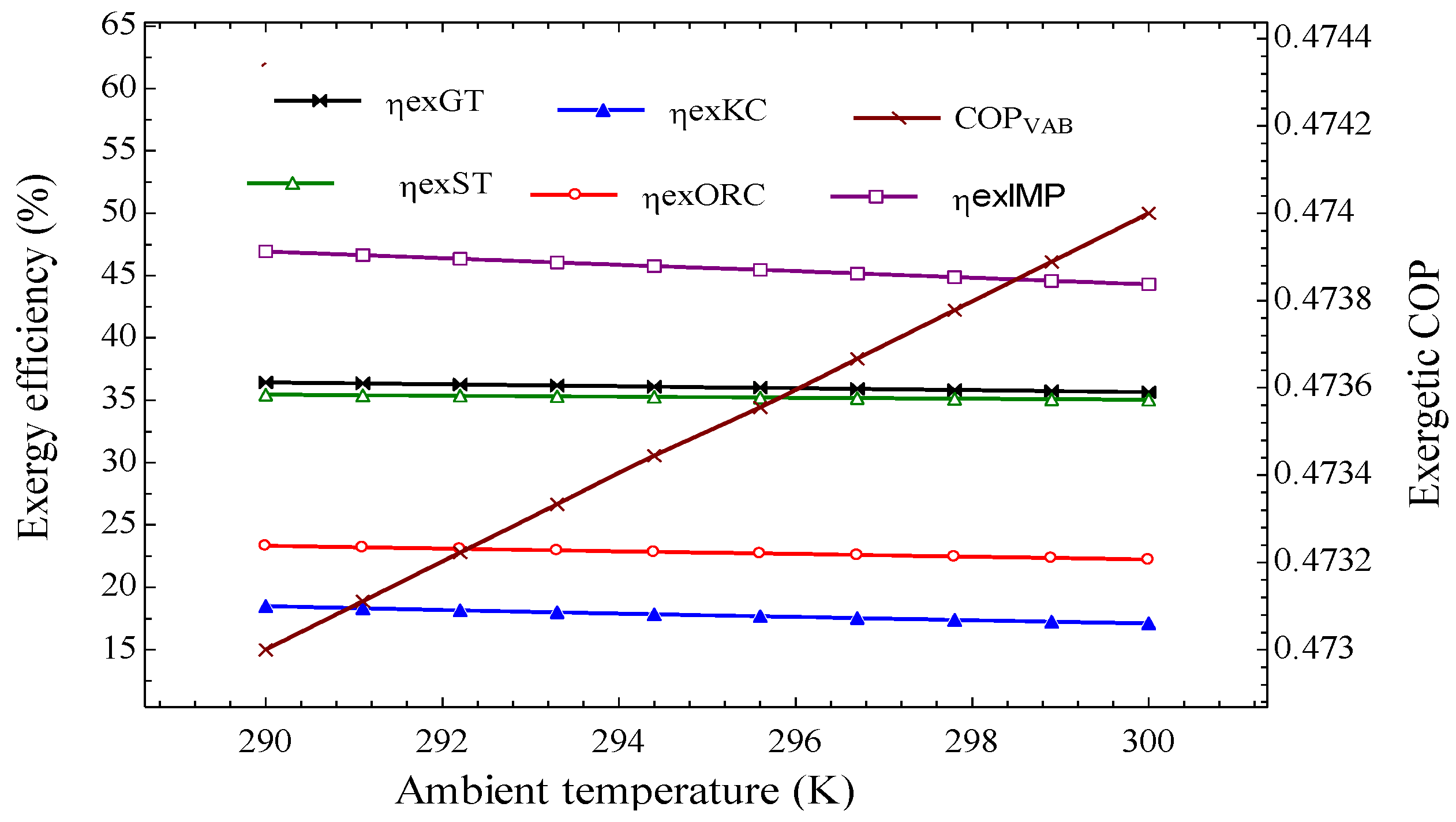
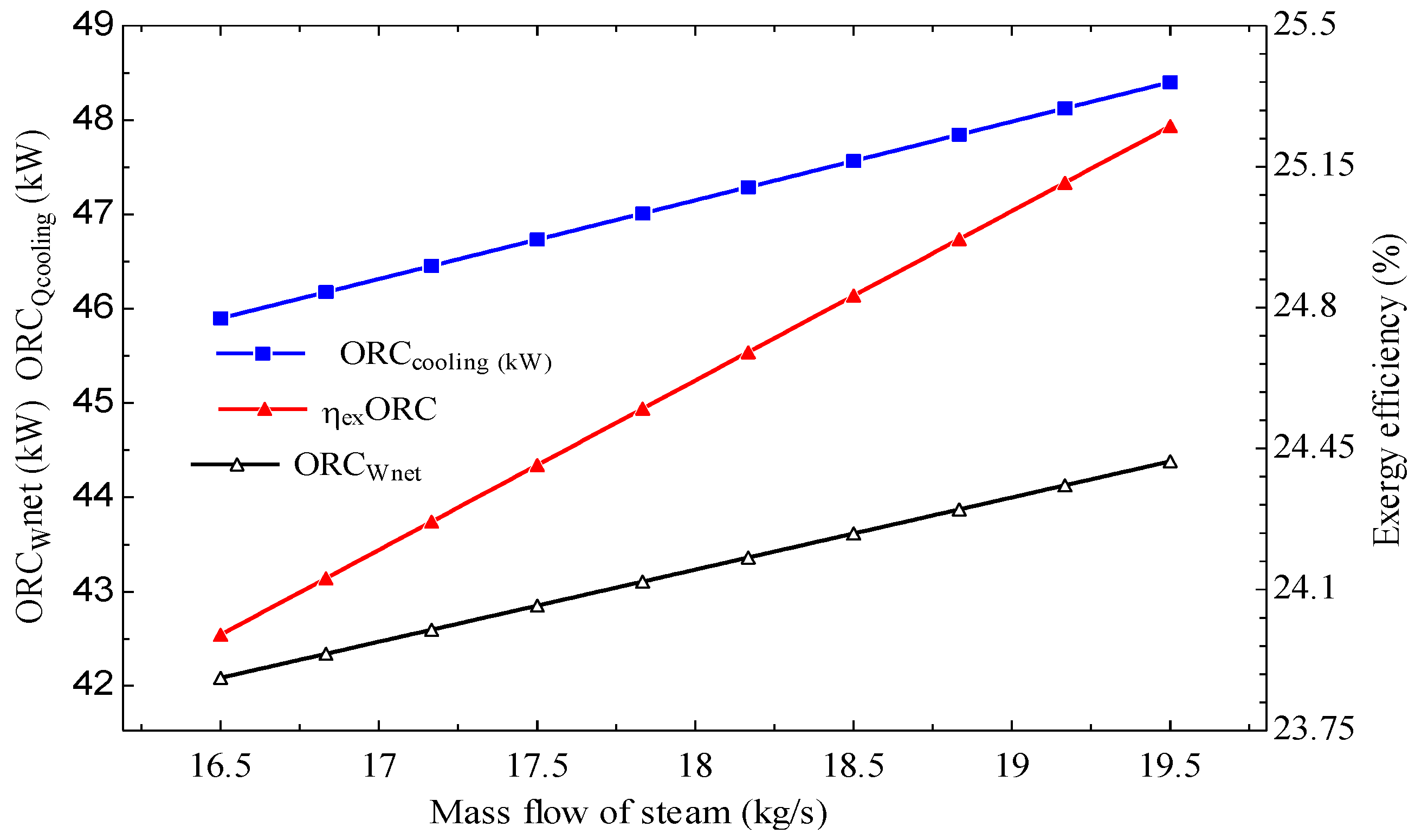
3.1.2. Parametric Analysis

Figure 2 depicts the performance of the subsystems and the IMP with variations in ambient temperature (AT). For an increase in AT between $290\le AT\le 300 K$, the exergy efficiency, ${\eta }_{ex}$, decreased by 6.8% for GT, 1.1% for the ORC, 1.2% for the KC, 1.9% for ST, and 2.97% for the IMP. The ORC and the Kalina cycles had the least decrease in ${\eta }_{ex}$, indicating small exergy destruction in these cycles, which is expected for low-grade temperature energy conversion systems. The variation in AT had no substantial effect in the exergetic COP of the VAB system.

The effect of the mass flow rate of steam (${\dot{m}}_{st}$) on the ORC performance is shown in Figure 3. The ${\eta }_{ex}$ increased by 4.99% for ${\dot{m}}_{st}\left(kg/s\right)$ within $16.5\le {\dot{m}}_{st}\le 19.5$. Similarly, the ${\dot{W}}_{net}$ increased by 5.2%, whereas the cooling load varied between $45.9\le {\dot{Q}}_{cooling}\le 48.4 \mathrm{kW}$.

Figure 4 presents the effect of adiabatic flame temperature, T_pz, on the specific CO₂ emission, and harmful fuel emission factor (F_EF). At 2000 K adiabatic flame temperature, the specific CO₂ emission was estimated at 140 kg/MWh, with about 60% increase in F_EF. Increase in Tpz favored F_EF and CO₂ yield, and was consequently harmful to the environment. The optimal value of the adiabatic flame temperature is, therefore, required to reduce environmental pollution.

Figure 5 shows the effect of the ratio of adiabatic flame temperature to ambient temperature ($T_{pz}/T_0$) on NOx and CO emissions. The measure of NOx and CO produced throughout the combustion process increases steadily with increasing T_pz/T₀, which is expected, as high combustion temperature favors NOx and CO formation through a dissociation process.

Figure 6 shows the variation in exergy efficiency, ${\eta }_{ex}$, on the sustainability indicators. An increase in ${\eta }_{ex}$ results in corresponding increases in EUE and SI. Additionally, ETI decreases for all values of ${\eta }_{ex}$. The trend of the indicators is analogous to other sustainability indicators found in the work of Owebor et al. [19].

3.2. Economic Evaluation

The results of the total exergoeconomic parameters for the subsystems are depicted in

Table 6. Exergoeconomic parameters for the gas turbine plant.

Component	${\dot{\mathit{C}}}_{\mathit{F}}$ ($/GJ)	${\dot{\mathit{C}}}_{\mathit{P}}$ ($/GJ)	${\dot{\mathit{E}}}_{\mathit{D}}$ (MW)	${\dot{\mathit{C}}}_{\mathit{D}}$ ($/hr.)	$\mathit{Z}$ ($/hr.)	$\mathit{\psi }$ (%)	$\mathit{Z}+{\dot{\mathit{C}}}_{\mathit{D}}$ ($/hr.)	${\mathit{f}}_{\mathit{k}}$ (%)	${\mathit{r}}_{\mathit{k}}$ (%)
GT CC	0.158	0.203	50.365	28.542	5.895	80.54	34.438	82.88	28.48
GT HEX	0.168	0.221	10.128	6.131	2.148	81.05	8.280	74.06	31.55
GT HPC	1.389	0.511	9.575	47.880	12.189	79.98	60.067	79.71	31.36
GT HPT	0.203	0.392	10.039	7.346	37.858	86.88	45.204	16.25	93.10
GT INTC	0.504	2.959	2.702	4.908	2.195	22.93	7.1023	69.10	487.10
GT LPC	0.339	0.504	2.883	3.513	12.189	90.12	15.703	22.38	48.67
GT LPT	0.169	0.353	8.871	5.372	41.693	88.92	47.064	11.42	108.88
GT REH	0.156	0.165	4.201	2.352	5.483	97.62	7.835	30.02	5.77

,

Table 7. Exergoeconomic parameters for the heat regenerative steam generator (HRSG).

Component	${\dot{\mathit{C}}}_{\mathit{F}}$ ($/GJ)	${\dot{\mathit{C}}}_{\mathit{P}}$ ($/GJ)	${\dot{\mathit{E}}}_{\mathit{D}}$ (MW)	${\dot{\mathit{C}}}_{\mathit{D}}$ ($/hr.)	$\mathit{Z}$ ($/hr.)	$\mathit{\psi }$ (%)	$\mathit{Z}+{\dot{\mathit{C}}}_{\mathit{D}}$ ($/hr.)	${\mathit{f}}_{\mathit{k}}$ (%)	${\mathit{r}}_{\mathit{k}}$ (%)
HRSG HPE	0.1681	0.495	0.297	0.1803	1.371	81.55	1.550	11.63	194.47
HRSG HPEV	0.1682	0.237	5.176	3.1334	1.195	77.23	4.329	72.38	40.90
HRSG LPE	0.1682	1.104	0.056	0.0342	1.167	86.32	1.201	2.85	556.36
HRSG LPEV	0.1681	0.489	5.432	3.2890	1.372	56.79	4.661	70.56	190.90
HRSG PUM	1.7352	17.752	0.022	0.1357	0.453	31.97	0.589	23.04	923.05

,

Table 8. Exergoeconomic parameters for the Kalina power cooling cycle.

Component	${\dot{\mathit{C}}}_{\mathit{F}}$ ($/GJ)	${\dot{\mathit{C}}}_{\mathit{P}}$ ($/GJ)	${\dot{\mathit{E}}}_{\mathit{D}}$ (MW)	${\dot{\mathit{C}}}_{\mathit{D}}$ ($/hr.)	$\mathit{Z}$ ($/hr.)	$\mathit{\psi }$ (%)	$\mathit{Z}+{\dot{\mathit{C}}}_{\mathit{D}}$ ($/hr.)	${\mathit{f}}_{\mathit{k}}$ (%)	${\mathit{r}}_{\mathit{k}}$ (%)
KCN5	27.145	52.848	0.0011	0.1119	0.0343	57.99	0.1462	76.54	94.69
KCN6	16.284	200.914	0.0687	4.0317	0.0805	8.255	4.1122	98.04	1133.81
KEV 1	9.619	12.819	0.0066	0.2194	1.7229	96.38	1.9424	11.30	33.27
KEV 2	26.533	1.0 × 10−6	0.0025	0.2390	0.4630	48.36	0.7020	34.04	100.00
KHEX 2	66.534	13.191	0.0004	0.0867	0.2746	73.04	0.3614	23.99	80.17
KHEX 3	27.148	145.76	0.0016	0.1611	0.1720	32.12	0.3332	48.36	436.91
KPUM 1	23.540	34.121	0.0001	0.0001	0.0405	99.95	0.0406	0.25	44.95
KSP 1	13.969	15.326	0.0098	0.4918	0.2986	94.31	0.7903	62.22	9.71
KSP 2	15.321	16.286	0.0004	0.0236	0.2654	99.49	0.2889	8.17	6.30
KTUB	15.317	23.530	2.0 × 10−5	0.0000	1.1942	99.99	1.1942	2.0 × 10−6	53.62
KVAL 1	15.324	26.238	0.0168	0.9301	0.0268	59.09	0.9569	97.20	71.22
KVAL 2	16.286	32.012	0.0002	0.0152	0.0230	72.24	0.0382	39.79	96.56
KALV 3	16.284	41.795	0.0043	0.2551	0.0212	40.88	0.2763	92.33	156.66

,

Table 9. Exergoeconomic parameters for the ORC power cooling cycle.

Component	${\dot{\mathit{C}}}_{\mathit{F}}$ ($/GJ)	${\dot{\mathit{C}}}_{\mathit{P}}$ ($/GJ)	${\dot{\mathit{E}}}_{\mathit{D}}$ (MW)	${\dot{\mathit{C}}}_{\mathit{D}}$ ($/hr.)	$\mathit{Z}$ ($/hr.)	$\mathit{\psi }$ (%)	$\mathit{Z}+{\dot{\mathit{C}}}_{\mathit{D}}$ ($/hr.)	${\mathit{f}}_{\mathit{k}}$ (%)	${\mathit{r}}_{\mathit{k}}$ (%)
ORC CON 2	20.664	114.089	2.5300	0.2166	0.016	18.70	0.232	93.017	452.11
ORC CON 3	10.755	81.846	0.0607	2.3527	0.066	13.46	2.418	97.261	661.00
ORC EVP 4	20.233	52.307	0.0755	5.5059	0.565	41.03	6.071	90.690	158.52
ORC EVP 5	16.559	3.0 × 10−6	0.0032	0.1917	0.269	28.84	0.461	41.579	100.00
ORC HEX 5	27.494	20.670	0.0004	0.0416	0.158	91.90	0.200	20.780	24.82
ORC PUM 4	27.551	50.028	2.0 × 10−7	0.0000	0.073	71.69	0.073	2.0 × 10−7	81.58
ORC TUB	20.673	27.563	2.0 × 10−6	0.0000	1.366	99.99	1.366	3.0 × 10−6	33.33
ORC VAL 6	20.663	24.918	0.0031	0.2290	0.005	83.30	0.234	97.687	20.59

,

Table 10. Exergoeconomic parameters for the steam turbine plant.

Component	${\dot{\mathit{C}}}_{\mathit{F}}$ ($/GJ)	${\dot{\mathit{C}}}_{\mathit{P}}$ ($/GJ)	${\dot{\mathit{E}}}_{\mathit{D}}$ (MW)	${\dot{\mathit{C}}}_{\mathit{D}}$ ($/hr.)	$\mathit{Z}$ ($/hr.)	$\mathit{\psi }$ (%)	$\mathit{Z}+{\dot{\mathit{C}}}_{\mathit{D}}$ ($/hr.)	${\mathit{f}}_{\mathit{k}}$ (%)	${\mathit{r}}_{\mathit{k}}$ (%)
ST CON	0.3801	0.317	0.8655	1.1846	1.721	60.07	2.905	40.77	16.60
ST FWH 1	0.3306	0.847	0.1093	0.1301	0.430	47.58	0.560	23.22	156.20
ST FWH 2	0.5711	0.699	1.4910	3.0655	0.573	94.06	3.639	84.23	22.40
ST PUM 1	1.7352	10.43	1.0 × 10−7	1.0 × 10−5	0.065	99.99	0.065	1.0 × 10−6	501.08
ST PUM 2	1.7345	7.977	1.0 × 10−7	1.0 × 10−5	0.147	99.99	0.147	1.0 × 10−6	359.90
ST PUM 3	1.7341	7.177	1.0 × 10−7	1.0 × 10−5	0.205	99.99	0.205	1.0 × 10−6	313.87
ST TUB	0.3178	1.734	1.0 × 10−6	2.0 × 10−4	0.817	99.99	0.817	1.0 × 10−5	445.63

and

Table 11. Summary of the exergoeconomic parameters for the vapor absorption system (VAB).

Component	${\dot{\mathit{C}}}_{\mathit{F}}$ ($/GJ)	${\dot{\mathit{C}}}_{\mathit{P}}$ ($/GJ)	${\dot{\mathit{E}}}_{\mathit{D}}$ (MW)	${\dot{\mathit{C}}}_{\mathit{D}}$ ($/hr.)	$\mathit{Z}$ ($/hr.)	$\mathit{\psi }$ (%)	$\mathit{Z}+{\dot{\mathit{C}}}_{\mathit{D}}$ ($/hr.)	${\mathit{f}}_{\mathit{k}}$ (%)	${\mathit{r}}_{\mathit{k}}$ (%)
VABA	13.200	57.132	0.0080	0.3790	0.0999	26.37	0.4789	79.14	332.82
VAB CON 4	68.982	217.240	0.0047	1.162	0.0290	32.29	1.1905	97.56	214.92
VABDE	13.200	57.132	0.0163	0.776	0.1499	26.37	0.9259	83.81	332.82
VAB EVP 3	4.657	1.0 × 10−5	0.0076	0.127	0.1861	31.51	0.3135	40.64	100.00
VAB HEX 4	58.580	102.335	0.0003	0.066	0.2117	84.94	0.2777	23.77	74.69
VAB PUM 7	23.527	150.988	2.0 × 10−6	0.0002	0.0008	100.00	0.0009	20.41	541.76
VAB VAL 4	9.577	66.704	0.0058	0.201	0.0058	13.89	0.2071	97.20	596.50
VAB VAL 5	13.380	68.978	0.0007	0.031	0.0073	14.30	0.0388	81.29	415.53

. The exergoeconomic factors ($f_k$) were estimated at 53.01%, 45.08%, 41.29%, 22.79%, 47.41%, and 20.11% for GT, HRSG, KC, ORC, ST, and VAB, respectively. Low $f_k$ values for a component signifies a high exergy destruction cost and equally connotes a high potential for improvement, whereas high $r_k$ denotes the potential for subsystem optimization. The combined effects of $f_k$ and $r_k$ showed that the gas turbine (GT) had the highest potentials for improvement, followed by the HRSG, ST, and KC, while the VAB and ORC had limited space for optimization.

Figure 7 shows the overall exergoeconomic data for the proposed integrated multi-generation plant. The figure shows that the overall exergoeconomic factor, $f_k$, and the relative cost difference, $r_k$, were estimated at 50.37% and 162.38%, respectively. However, the study indicates that only 49.37% of the total cost was connected with the exergy destruction, following the 50.37% overall $f_k$ for the IMP.

Table 12. Economic results for the IMP.

Parameter	Symbol	Units	Value
Cost of IMP equipment	$Z_{PPEC}$	$\$\times {10}^6$	9.43
Life cycle cost (LCC)	$Z_{LCC}$	$\$\times {10}^6$	1.575
Daily energy production	$E_{DP}$	$\mathrm{MWh}/\mathrm{d}$	4413.84
Annual energy production	$E_{AP}$	$\mathrm{MWh}/\mathrm{y}$	$1.61\times {10}^6$
The unit cost of energy	$UCOE$	$/kW	0.0166
Annualized life cycle cost	$Z_{ALCC}$	$\$\times {10}^4$	2.6748
Break-even point	$BEP$	year	4.0

presents other economic data of the IMP. The proposed IMP had $1.575 million as the life cycle cost, whereas $9.43 million was obtained for the cost of the IMP equipment, with a breakeven point (BEP) estimated at 4 years. The value of 0.0166 $/kWh was obtained for the unit cost of electricity (UCOE) of the proposed IMP, which was far less than the average cost of electricity (0.067 $/kWh) from the national grid of Nigeria. The low value of the UCOE of the proposed IMP was an indication that the proposed plant would have an economic advantage over the existing power plants in the country.

The cost of emissions was related to the mass of emissions per annum and is shown in Figure 8. The unit cost of emissions was taken as 0.02086, 0.024, and 6.853 $/kg for NOx, CO, and CO₂, respectively [48]. The emission cost of CO was remarkably low, since the operation of the combustion chambers was at values above the air-fuel stoichiometric requirements. Furthermore, the choice of the turbine inlet temperature of 1300 K in the initial data consideration, assisted in severely cutting down the emissions as well as its associated cost. The cost associated with CO and NOx emissions were directly governed by the adiabatic flame temperature (AFT) and appeared nearly constant between the AFTs of 1200 and 2200 K. However, the data points showed that the cost from CO emissions were negligible when the AFT was between 1200 and 2295 K. For the same AFT range, NOx emissions cost was high, about 588.2$ at 2295 K. Therefore, for small emissions, cost from NOx and CO, AFTs between 1200 and 1400 are recommended. Additionally, the emissions cost of CO₂ was 338.9 $ per annum and remained constant and independent of the AFT, from its defining relationship.

4. Optimum Parameters

The objective functions considered include the overall exergy efficiency and the overall cost rate of the product. The exergy efficiency is to be maximized, whereas the overall cost rate is to be minimized. Added to the overall cost rate equation of the plant is the cost of pollution damage. The objective functions are presented as follows:

$${\psi }_{overall}=\frac{\left\{{\dot{E}}_{W_{LPT}}+{\dot{E}}_{W_{HPT}}+{\dot{E}}_{W_{ST}}+{\dot{E}}_{W_{KT}}+{\dot{E}}_{W_{ORCT}}+{\dot{E}}_{R_{Kalina}}+{\dot{E}}_{R_{VAS}}+{\dot{E}}_{R_{ORC}}\right\}-\left\{{\dot{E}}_{W_{LPC}}+{\dot{E}}_{W_{HPC}}+{{\displaystyle \sum }}_{i=1}^6{\dot{E}}_{W_{P_i}}\right\}}{A_d}$$

(74)

where $\psi$ is the overall exergy efficiency, and the denominator ($A_d$) of Equation (74) is expressed in Equation (75)

$$A_d=\Vert \left[1-\frac{T_0}{T_6}\right]{\dot{Q}}_6+\left[1-\frac{T_0}{T_9}\right]{\dot{Q}}_9\Vert$$

(75)

where ${\dot{Q}}_6$ and ${\dot{Q}}_9$ are heat inputs into the combustion chamber and the supplemental firing process (reheater)—see Figure 1. The total cost rate of the system and the cost due to environmental impact are presented in Equations (76) and (77) [48]. The components of optimization function parameters, objective functions, constraints, and performance index are presented in

Table 13. Components of optimization functions and parameters.

Performance Index	Optimization Function	Decision Variables	Optimization Constraints
$W_{LPC}$	${\dot{m}}_1{c}_p\frac{T_1}{{\eta }_{LPC}}\left[{\left(r_p\right)}^k-1\right]$	${\eta }_{LPC}, r_p$	$0.75\le LPC\le 0.89$
$W_{HPC}$	${\dot{m}}_3{c}_p\frac{T_3}{{\eta }_{HPC}}\left[{\left(r_p\right)}^k-1\right]$	${\eta }_{LPC}, r_p$	$0.75\le LPC\le 0.89$
$W_{LPT}$	${\dot{m}}_{10}{c}_p{T}_{10}{\eta }_{LPT}\left|1-\frac{1}{{\left(r_p\right)}^k}\right|$	${\eta }_{LPC}, r_{p, }{T}_{10}$	$0.75\le LPC\le 0.8$, 8 $\le r_p\le 16$,$1150\le T_{10}\le 1250$
$W_{HPT}$	${\dot{m}}_7{c}_p{T}_7{\eta }_{HPT}\left|1-\frac{1}{{\left(r_p\right)}^k}\right|$	${\eta }_{LPC}, r_{p, }{T}_7$	$0.75\le LPC\le 0.8$, 8 $\le r_p\le 16$, $1150\le T_7\le 1250 K$
$W_{ST}$	${\dot{m}}_{14}\left|h_{14}-h_{21}\right|$ $+\left|{\dot{m}}_{14}-{\dot{m}}_{21}\right|.\left|h_{21}-h_{18}\right|$ $+\left|{\dot{m}}_{14}-{\dot{m}}_{21}-{\dot{m}}_{18}\right|.\left|h_{18}-h_{15}\right|$	$P_{14}, P_{21}, P_{18}, P_{15}$, pressure at $h_{14}$, $T_{14}$, pressure at $s_{14}$, $h_{21}$, pressure at $s_{14}$, $h_{18}$, pressure at $s_{14}$, $h_{15}$	$3100\le h_{14}\le 3200$, 2740$\le h_{21}\le 2555$, $2530\le h_{18}\le 2555$, 2130$\le h_{15}\le 2145$
$W_{Kal. Turb}$	${\dot{m}}_{28}\left|h_{28}-h_{29}\right|+$ $\left|{\dot{m}}_{28}-{\dot{m}}_{29}\right|.\left|h_{29}-h_{33}\right|$	$P_{28},$ pressure at $T_{28}$, $h_{28}$	$435\le T_{28}\le 439 \mathrm{K}$
$W_{ORC. Turb}$	${\dot{m}}_{39}\left|h_{39}-h_{41}\right|$	$P_{39}, P_{41}, \mathrm{Pressure} \mathrm{at} X_{39}, h_{39}, T_{39}$, $\mathrm{Pressure} \mathrm{at} X_{39}, h_{41}, s_{39}$	$2130\le h_{39}\le 2170$, $1950\le h_{41}\le 1980$
$Q_{EVP5}$	${\dot{m}}_{31}\left|h_{32}-h_{31}\right|$	$T_{31}$	$T_{61}$, −3 and −1.5 °C
$Q_{EVP3}$	${\dot{m}}_{60}\left|h_{61}-h_{60}\right|$	$T_{60}$	$270\le T_{60}\le 282$
$Q_{EVP2}$	${\dot{m}}_{44}\left|h_{45}-h_{44}\right|$	$T_{44}$	$T_{44}$, −5.8 and −1.5 °C
${\dot{C}}_{ost,}Total$	${\dot{C}}_{fuel}+{\dot{C}}_{env.}+{\displaystyle {\displaystyle \sum }_k}{\dot{Z}}_k$	All listed parameters

.

$${\dot{C}}_{Tot}={\dot{C}}_{fuel}+{\dot{C}}_{env.}+{{\displaystyle \sum }}_k{\dot{Z}}_k$$

(76)

$${\dot{C}}_{env}=C_{N{O}_x}{\dot{m}}_{N{O}_x}+C_{C{O}_2}{\dot{m}}_{C{O}_2}+C_{CO}{\dot{m}}_{CO}$$

(77)

where the unit damage costs $C_{N{O}_x}$, $C_{C{O}_2}$, and $C_{CO}$ were taken as 0.02086 $/kg, 6.853 $/kg, and 0.024 $/kg, respectively, according to [48].

The genetic algorithm (GA) was used because of its ability to handle multi-objective and multi-variable problems. Ninety sets of Pareto-frontiers from the genetic algorithm (GA) were established and compiled, based on the objective functions and the corresponding constraints. The 19th Pareto-front corresponded to the maximum exergy efficiency and least-cost rate of 45.32% and 125.84 $/hr, respectively. The equivalent parameters of the system at this point existed at—compression ratio (8), LPC (0.88), HPC (0.88), LPT (0.88), and HPT (0.88) isentropic efficiencies. Similarly, the intercooler outlet temperature, CC inlet temperature, supplemental firing (reheater) temperature were estimated at 376.7 K, 1150 K, and 1250.3 K, respectively. The optimum inlet pressures of the ORC and KC were obtained as 16.27 kPa and 20 kPa, respectively, corresponding to the obtained optimum operating enthalpies. The specific emissions at the optimal operating parameters were estimated at $120.34$, 2.9 × 10⁻⁷, and 0.213 kg/MWh for CO₂, CO, and NOx, respectively, with enhanced environmental emissions of 1.55% for CO₂, 4.23% for NOx, and 3.45% for CO.

5. Conclusions

The present study presents integrated multi-generation system by retrofitting an in-service FRAME 9E gas turbine power plant located in Calabar, Nigeria. The in-service gas turbine plant, fired by natural gas, was retrofitted with a gas turbine (GT), steam turbine (ST), organic Rankine cycle (ORC) for cooling and power production, a modified Kalina cycle (KC) for power production and cooling, and a vapor absorption system (VAB) for cooling. The retrofitted plant was fired by natural gas, with a biomass-based syngas supplemental firing. The proposed system was prompted to solve the energy-supply–climate-change dilemma, by reducing emission and increasing the useful energy output of the existing FRAME 9E gas turbine plant. The operational data of the gas turbine were used as a basis to conduct the thermo-enviroeconomic analysis. The results obtained are summarized as follows:

• The overall power output for the subsystem was calculated at 148.73 MW for GT, 35.91 MW for ST, 42.82 kW for ORC, and 36.27 kW for the Kalina power-cooling cycle. The total power output generated by the IMP was 183 MW, which was about 1.2 times greater than the GT plant, stood alone.
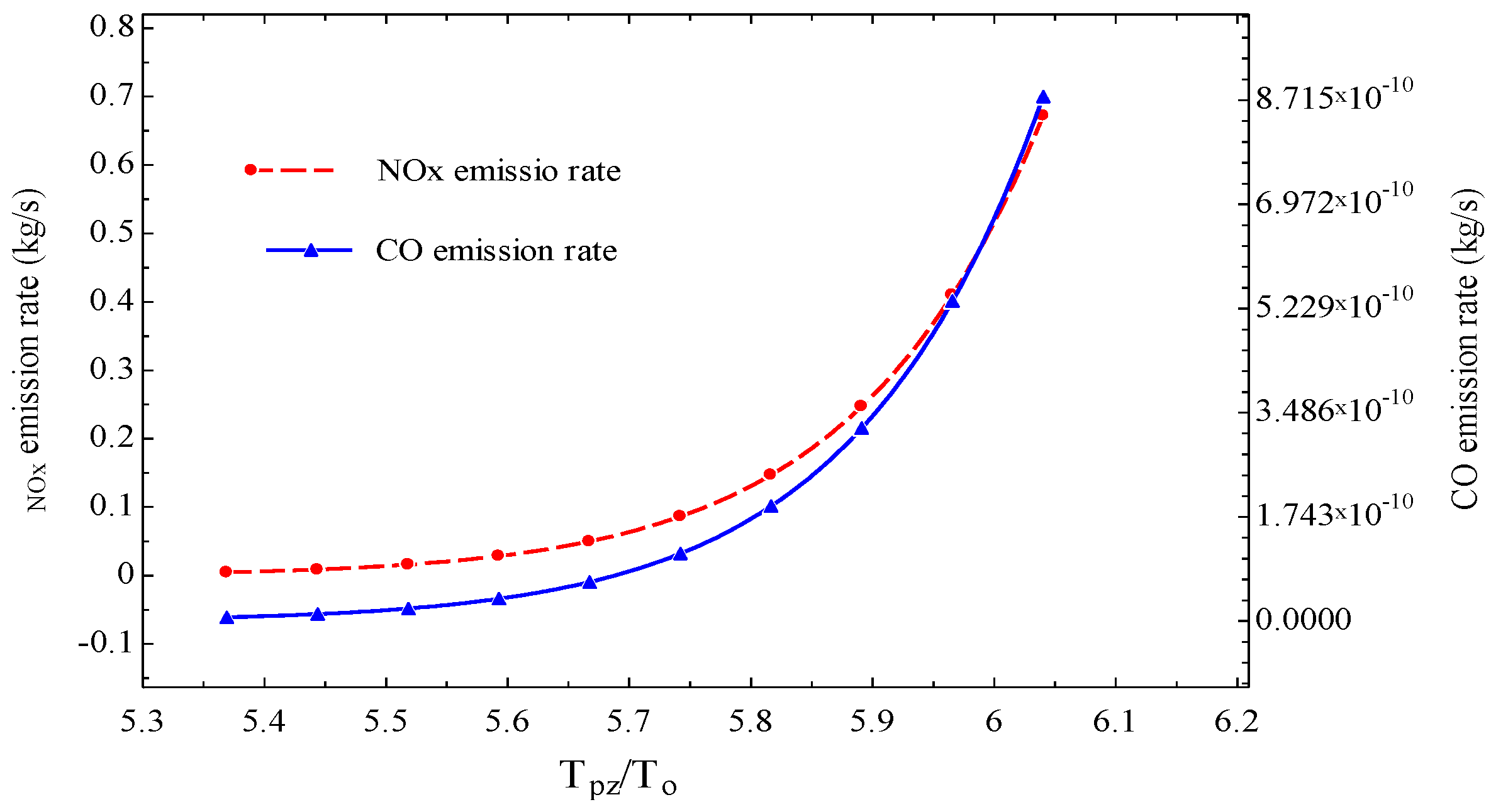
• The energy and exergy efficiencies for the IMP were obtained at 61.5 and 44.22%, respectively, while the environmental parameters such as harmful emission factor, specific CO₂ emission, NOx and CO values, existed at $122.2 {\mathrm{kg}}_{{\mathrm{CO}}_2}/\mathrm{MWh}$, 3.0 × 10⁻⁷$\mathrm{kg}/\mathrm{s}$, and 0.222 $\mathrm{kg}/\mathrm{s}$, in that order.
• The novel sustainability indicators applied to this study—exergetic utility exponent (EUE) and exergo-thermal index (ETI) for the IMP were calculated at 0.7335 and 0.675. These values were found to be improved, as compared to the stand-alone GT plant, which connotes good conversion efficiency.
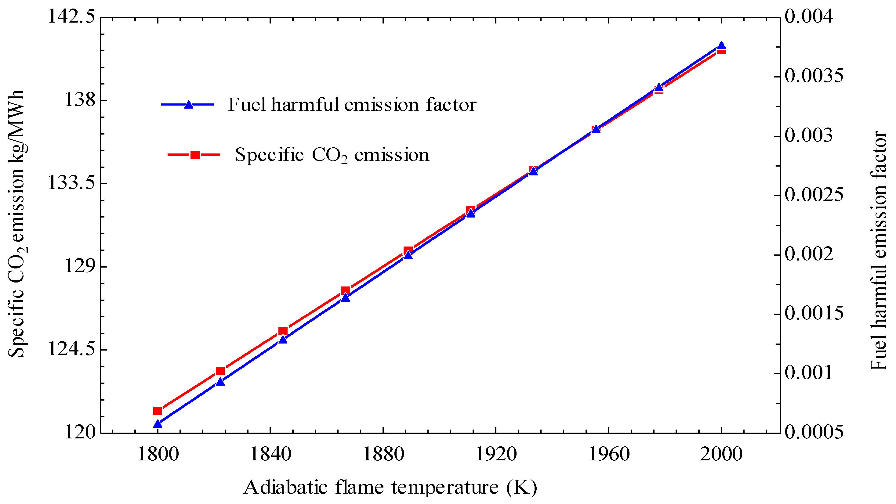
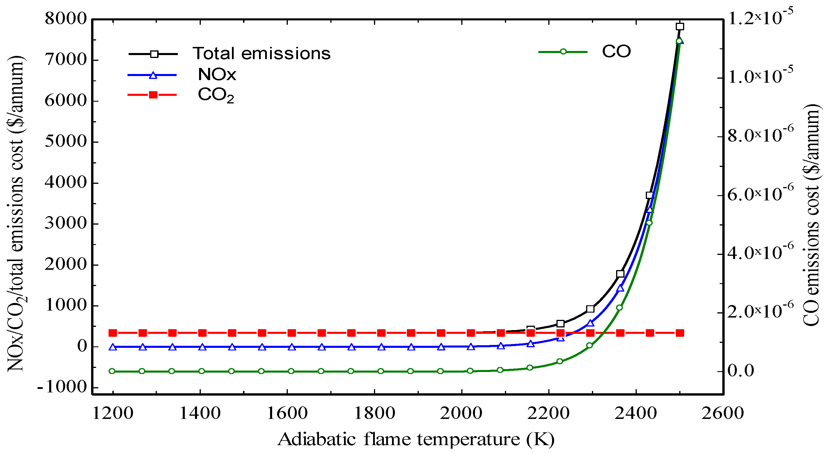
• The cost of CO emissions was found negligible at an adiabatic flame temperature of 1200 and 2295 K, while for the same temperature range NOx and CO₂ emission cost were maximum, approximated at 588.2 and 338.9$ per annum, respectively.
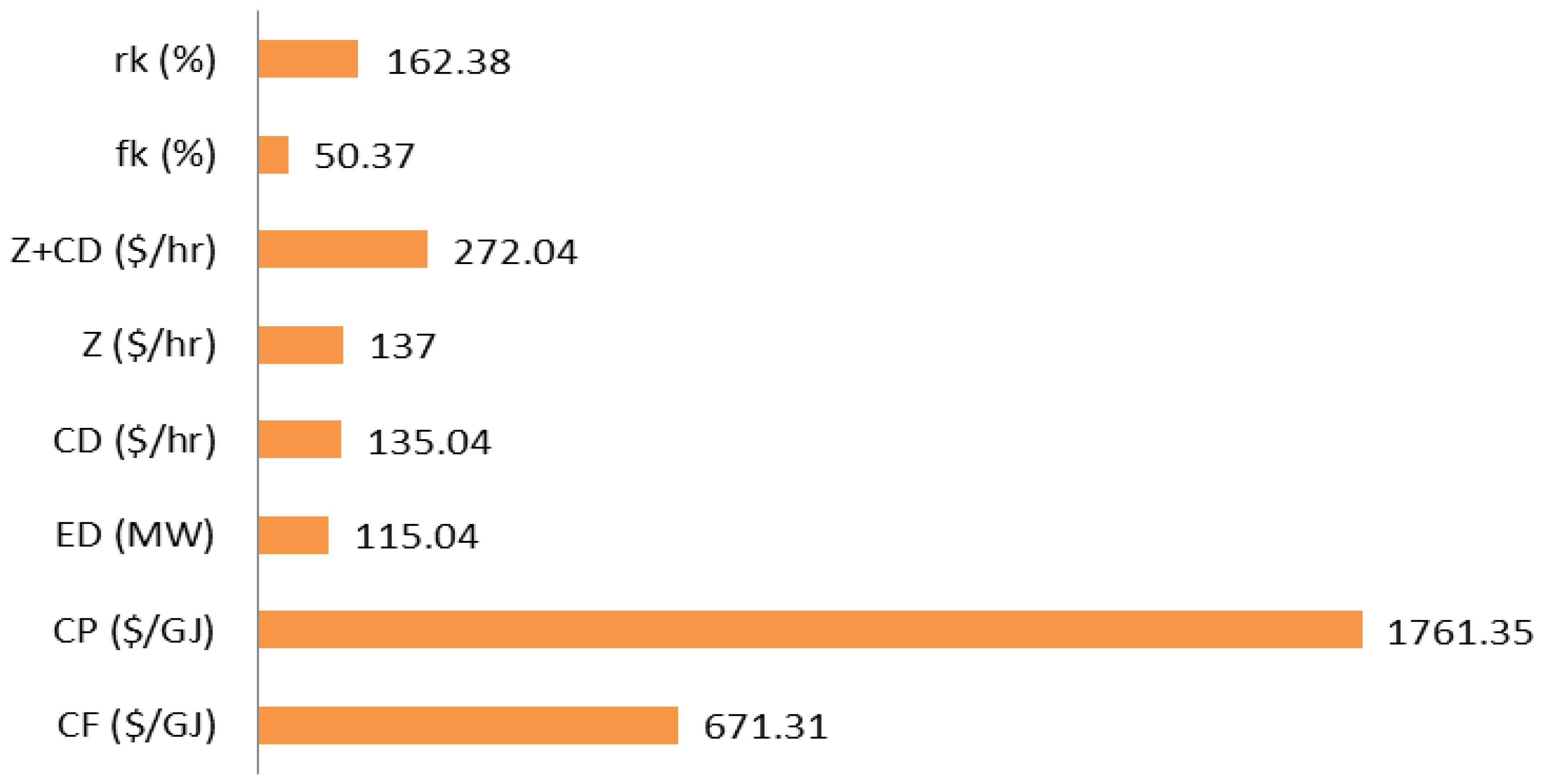
• Life cycle cost of $1.58 million was achieved, with a BEP (or payback period) of four years. The UCOE of 0.0166 $/kWh was obtained with exergoeconomic factor of 50.37% for the IMP. Additionally, 125.83 $/hr cost and 45.32% exergy efficiency were achieved at the optimum operating condition.
• The present study will support policymakers and decision-makers to drive sustainable energy access to meet both the Paris Agreement and Sustainable Development Goals agenda in the context of Nigeria’s energy landscape and the global south.
• The proposed system is very important to drive the current energy transition crisis caused by the COVID-19 pandemic shock in the energy sector.

References

1. Flores, W.; Bustamante, B.; Pino, H.N.; Al-Sumaiti, A.S.; Rivera-Rodríguez, S.R. A National Strategy Proposal for Improved Cooking Stove Adoption in Honduras: Energy Consumption and Cost-Benefit Analysis. Energies 2020, 13, 921. [Google Scholar] [CrossRef] [Green Version]
2. Steffen, B.; Egli, F.; Pahle, M.; Schmidt, T.S. Navigating the Clean Energy Transition in the COVID-19 Crisis. Joule 2020, 4, 1137–1141. [Google Scholar] [CrossRef]
3. Carvalho, M.; Bandeira de Mello Delgado, D.; de Lima, K.M.; de Camargo Cancela, M.; dos Siqueira, C.A.; de Souza, D.L.B. Effects of the COVID-19 pandemic on the Brazilian electricity consumption patters. Int. J. Energy Res. 2020, e5877. [Google Scholar]
4. Kanda, W.; Kivimaa, P. What opportunities could the COVID-19 outbreak offer for sustainability transitions research on electricity and mobility? Energy Res. Soc. Sci. 2020, 68, 101666. [Google Scholar] [CrossRef]
5. Marques, A.D.S.; Carvalho, M.; Lourenço, A.B.; Dos Santos, C.A.C. Energy, exergy, and exergoeconomic evaluations of a micro-trigeneration system. J. Braz. Soc. Mech. Sci. Eng. 2020, 42, 1–16. [Google Scholar] [CrossRef]
6. Quadrelli, R.; Peterson, S. The energy–climate challenge: Recent trends in CO2 emissions from fuel combustion. Energy Policy 2007, 35, 5938–5952. [Google Scholar] [CrossRef]
7. Newman, P. COVID, CITIES and CLIMATE: Historical Precedents and Potential Transitions for the New Economy. Urban Sci. 2020, 4, 32. [Google Scholar] [CrossRef]
8. Rezk, H.; Alghassab, M.; Ziedan, H.A. An Optimal Sizing of Stand-Alone Hybrid PV-Fuel Cell-Battery to Desalinate Seawater at Saudi NEOM City. Processes 2020, 8, 382. [Google Scholar] [CrossRef] [Green Version]
9. Alghassab, M. Performance Enhancement of Stand-Alone Photovoltaic Systems with household loads. In Proceedings of the 2nd International Conference on Computer Applications & Information Security (ICCAIS), Riyadh, Saudi Arabia, 1–3 May 2019; pp. 1–6. [Google Scholar] [CrossRef]
10. Ghaebi, H.; Parikhani, T.; Rostamzadeh, H.; Farhang, B. Thermodynamic and thermoeconomic analysis and optimization of a novel combined cooling and power (CCP) cycle by integrating of ejector refrigeration and Kalina cycles. Energy 2017, 139, 262–276. [Google Scholar] [CrossRef]
11. Mondol, J.D.; Carr, C. Techno-economic assessments of advanced Combined Cycle Gas Turbine (CCGT) technology for the new electricity market in the United Arab Emirates. Sustain. Energy Technol. Assess. 2017, 19, 160–172. [Google Scholar] [CrossRef]
12. Bicer, Y.; Dincer, I. Development of a new solar and geothermal based combined system for hydrogen production. Sol. Energy 2016, 127, 269–284. [Google Scholar] [CrossRef]
13. Ozturk, M.; Dincer, I. Thermodynamic analysis of a solar-based multi-generation system with hydrogen production. Appl. Therm. Eng. 2013, 51, 1235–1244. [Google Scholar] [CrossRef]
14. Mohan, G.; Dahal, S.; Kumar, U.; Martin, A.; Kayal, H. Development of Natural Gas Fired Combined Cycle Plant for Tri-Generation of Power, Cooling and Clean Water Using Waste Heat Recovery: Techno-Economic Analysis. Energies 2014, 7, 6358–6381. [Google Scholar] [CrossRef] [Green Version]
15. Khalid, F.; Dincer, I.; Rosen, M.A. Energy and exergy analyses of a solar-biomass integrated cycle for multigeneration. Sol. Energy 2015, 112, 290–299. [Google Scholar] [CrossRef]
16. Islam, S.; Dincer, I.; Yilbas, B.S. Energetic and exergetic performance analyses of a solar energy-based integrated system for multigeneration including thermoelectric generators. Energy 2015, 93, 1246–1258. [Google Scholar] [CrossRef]
17. Al-Ali, M.; Dincer, I. Energetic and exergetic studies of a multigenerational solar–geothermal system. Appl. Therm. Eng. 2014, 71, 16–23. [Google Scholar] [CrossRef]
18. Arafat, H.A.; Jijakli, K. Modeling and comparative assessment of municipal solid waste gasification for energy production. Waste Manag. 2013, 33, 1704–1713. [Google Scholar] [CrossRef]
19. Owebor, K.; Oko, C.; Diemuodeke, E.; Ogorure, O. Thermo-environmental and economic analysis of an integrated municipal waste-to-energy solid oxide fuel cell, gas-, steam-, organic fluid- and absorption refrigeration cycle thermal power plants. Appl. Energy 2019, 239, 1385–1401. [Google Scholar] [CrossRef]
20. Bonforte, G.; Buchgeister, J.; Manfrida, G.; Petela, K. Exergoeconomic and exergoenvironmental analysis of an integrated solar gas turbine/combined cycle power plant. Energy 2018, 156, 352–359. [Google Scholar] [CrossRef]
21. Khalid, F.; Dincer, I.; Rosen, M.A. Techno-economic assessment of a renewable energy based integrated multigeneration system for green buildings. Appl. Therm. Eng. 2016, 99, 1286–1294. [Google Scholar] [CrossRef]
22. Karellas, S.; Braimakis, K. Energy–exergy analysis and economic investigation of a cogeneration and trigeneration ORC–VCC hybrid system utilizing biomass fuel and solar power. Energy Convers. Manag. 2016, 107, 103–113. [Google Scholar] [CrossRef]
23. Boyaghchi, F.A.; Heidarnejad, P. Thermoeconomic assessment and multi objective optimization of a solar micro CCHP based on Organic Rankine Cycle for domestic application. Energy Convers. Manag. 2015, 97, 224–234. [Google Scholar] [CrossRef]
24. Parham, K.; Alimoradiyan, H.; Assadi, M. Energy, exergy and environmental analysis of a novel combined system producing power, water and hydrogen. Energy 2017, 134, 882–892. [Google Scholar] [CrossRef]
25. Suleman, F.; Dincer, I.; Agelin-Chaab, M. Development of an integrated renewable energy system for multigeneration. Energy 2014, 78, 196–204. [Google Scholar] [CrossRef]
26. Hassoun, A.; Dincer, I. Analysis and performance assessment of a multigenerational system powered by Organic Rankine Cycle for a net zero energy house. Appl. Therm. Eng. 2015, 76, 25–36. [Google Scholar] [CrossRef]
27. Gadhamshetty, V.; Nirmalakhandan, N.; Myint, M.; Ricketts, C. Improving Air-Cooled Condenser Performance in Combined Cycle Power Plants. J. Energy Eng. 2006, 132, 81–88. [Google Scholar] [CrossRef]
28. Odewale, S.A.; Sonibare, J.A.; Jimoda, L.A. Electricity sector’s contribution to greenhouse gas concentration in Nigeria. Manag. Environ. Qual. Int. J. 2017, 28, 917–929. [Google Scholar] [CrossRef]
29. Bicer, Y.; Dincer, I. Development of a multigeneration system with underground coal gasification integrated to bitumen extraction applications for oil sands. Energy Convers. Manag. 2015, 106, 235–248. [Google Scholar] [CrossRef]
30. Knudsen, T.; Clausen, L.R.; Haglind, F.; Modi, A. Energy and exergy analysis of the Kalina cycle for use in concentrated solar power plants with direct steam generation. Energy Procedia 2014, 57, 361–370. [Google Scholar] [CrossRef] [Green Version]
31. Rashidi, J.; Ifaei, P.; Esfahani, I.J.; Ataei, A.; Yoo, C. Thermodynamic and economic studies of two new high efficient power-cooling cogeneration systems based on Kalina and absorption refrigeration cycles. Energy Convers. Manag. 2016, 127, 170–186. [Google Scholar] [CrossRef]
32. Palacios-Bereche, R.; Gonzales, R.; Nebra, S.A. Exergy calculation of lithium bromide-water solution and its application in the exergetic evaluation of absorption refrigeration systems LiBr-H2O. Int. J. Energy Res. 2010, 36, 166–181. [Google Scholar] [CrossRef]
33. Koroneos, C.; Lykidou, S. Equilibrium modelling for a downdraft biomass gasifier for cotton stalks biomass in comparison with experimental data. J. Chem. Eng. Mater. Sci. 2011, 2, 61–68. [Google Scholar]
34. Gulder, O.L. Flame Temperature Estimation of Conventional and Future Jet Fuels. J. Eng. Gas Turbines Power 1986, 108, 376–380. [Google Scholar] [CrossRef]
35. Oyedepo, S.O.; Fagbenle, R.O.; Adefila, S.S.; Alam, M.M. Thermoeconomic and thermoenvironmic modeling and analysis of selected gas turbine power plants in Nigeria. Energy Sci. Eng. 2015, 3, 423–442. [Google Scholar] [CrossRef] [Green Version]
36. Ahmadi, P.; Dincer, I. Thermodynamic and exergoenvironmental analyses, and multi-objective optimization of a gas turbine power plant. Appl. Therm. Eng. 2011, 31, 2529–2540. [Google Scholar] [CrossRef]
37. Lazzaretto, A.; Tsatsaronis, G. SPECO: A systematic and general methodology for calculating efficiencies and costs in thermal systems. Energy 2006, 31, 1257–1289. [Google Scholar] [CrossRef]
38. Farshi, L.G.; Mahmoudi, S.; Rosen, M.A. Exergoeconomic comparison of double effect and combined ejector-double effect absorption refrigeration systems. Appl. Energy 2013, 103, 700–711. [Google Scholar] [CrossRef]
39. Jing, Y.; Li, Z.; Liu, L.; Lu, S. Exergoeconomic Assessment of Solar Absorption and Absorption–Compression Hybrid Refrigeration in Building Cooling. Entropy 2018, 20, 130. [Google Scholar] [CrossRef] [Green Version]
40. Oko, C.; Diemuodeke, E.; Omunakwe, E.; Nnamdi, E. Design and Economic Analysis of a Photovoltaic System: A Case Study. Int. J. Renew. Energy Dev. 2012, 1, 65–73. [Google Scholar] [CrossRef]
41. Soltani, S.; Athari, H.; Rosen, M.A.; Mahmoudi, S.M.S.; Morosuk, T. Thermodynamic analyses of biomass gasification integrated externally fired, post-firing and dual-fuel combined cycles. Sustainability 2015, 7, 1248–1262. [Google Scholar] [CrossRef] [Green Version]
42. Ahmadi, P.; Dincer, I.; Rosen, M.A. Development and assessment of an integrated biomass-based multi-generation energy system. Energy 2013, 56, 155–166. [Google Scholar] [CrossRef]
43. Abam, F.; Ekwe, E.; Effiom, S.; Ndukwu, M. A comparative performance analysis and thermo-sustainability indicators of modified low-heat organic Rankine cycles (ORCs): An exergy-based procedure. Energy Rep. 2018, 4, 110–118. [Google Scholar] [CrossRef]
44. Yilmaz, F.; Ozturk, M.; Selbas, R. Development and techno-economic assessment of a new biomass-assisted integrated plant for multigeneration. Energy Convers. Manag. 2019, 202, 112154. [Google Scholar] [CrossRef]
45. Safari, F.; Dincer, I. Development and analysis of a novel biomass-based integrated system for multigeneration with hydrogen production. Int. J. Hydrogen Energy 2019, 44, 3511–3526. [Google Scholar] [CrossRef]
46. Bamisile, O.; Huang, Q.; Dagbasi, M.; Alowolodu, O.; Williams, N. Development and Assessment of Renewable Energy–Integrated Multigeneration System for Rural Communities in Nigeria: Case Study. J. Energy Eng. 2020, 146, 05020001. [Google Scholar] [CrossRef]
47. Yilmaz, F.; Ozturk, M.; Selbas, R. Design and thermodynamic assessment of a biomass gasification plant integrated with Brayton cycle and solid oxide steam electrolyzer for compressed hydrogen production. Int. J. Hydrogen Energy 2020. [Google Scholar] [CrossRef]
48. Soltani, S.; Mahmoudi, S.; Yari, M.; Morosuk, T.; Rosen, M.; Zare, V. A comparative exergoeconomic analysis of two biomass and co-firing combined power plants. Energy Convers. Manag. 2013, 76, 83–91. [Google Scholar] [CrossRef]
Figure 1. The proposed integrated multi-generation plant. Note: Numbers represent inlet and exit states.
Energies 13 06018 g001
Figure 2. Effect of ambient temperature (AT) variations on the exergy efficiency of the subsystems and the IMP.
Energies 13 06018 g002
Figure 3. Effect of mass flow rate of steam on exergy efficiency, network, and cooling load of the ORC system.
Energies 13 06018 g003
Figure 4. Effect of adiabatic flame temperature on CO2 emission and FEF.
Energies 13 06018 g004
Figure 5. Effect of T p z / T 0 ratio on formation rates of NOx and CO.
Energies 13 06018 g005
Figure 6. Change in exergy efficiency on sustainability indicators.
Energies 13 06018 g006
Figure 7. Exergoeconomic parameters for the IMP.
Energies 13 06018 g007
Figure 8. Effect of adiabatic flame temperature on cost of emissions.
Energies 13 06018 g008