Article

Study of the Radar Cross-Section of Turbofan Engine with Biaxial Multirotor Based on Dynamic Scattering Method

School of Aeronautic Science and Engineering, Beihang University, Beijing 100191, China
*
Author to whom correspondence should be addressed.
Energies 2020, 13(21), 5802; https://doi.org/10.3390/en13215802
Submission received: 29 September 2020 / Revised: 25 October 2020 / Accepted: 2 November 2020 / Published: 5 November 2020
(This article belongs to the Special Issue Advances in Spark-Ignition Engines)

Abstract

:
With the continuous advancement of rotor dynamic electromagnetic scattering research, the radar cross-section (RCS) of turbofan engines has attracted more and more attention. In order to solve the electromagnetic scattering characteristics of a biaxial multirotor turbofan engine, a dynamic scattering method (DSM) based on dynamic simulation and grid transformation is presented, where the static RCS of the engine and its components is calculated by physical optics and physical theory of diffraction. The results show that the electromagnetic scattering of the engine is periodic when the engine is working stably, while the rotors such as fans and turbines are the main factors affecting the dynamic electromagnetic scattering and the ducts greatly increase the overall RCS level of the engine. The proposed DSM is effective and efficient for studying the dynamic electromagnetic scattering characteristic of the turbofan engine.

Graphical Abstract

1. Introduction

Stealth characteristics of aircraft engine intake and exhaust systems have been research hotspots, including infrared radiation, electromagnetic scattering, and noise [1,2]. In the face of the need for a comprehensive stealth design, the study of radar scattering characteristics of the turbofan engine is also receiving attention [3]. Therefore, the calculation of engine electromagnetic scattering has important practical significance for the stealth performance evaluation of the aircraft in the front-rear direction.
Turbofan engines usually consist of a compressor, combustion chamber, high-pressure turbine, low-pressure turbine, and exhaust system [4,5], which makes its electromagnetic scattering characteristics extremely complicated [6]. The engine intake contributes to the forward radar cross-section (RCS) of the aircraft [7] and the entire airflow duct creates complex reflections of the electromagnetic waves [8,9]. In general, physical optics (PO) [3], iterative physical optics [6], and method of moment (MOM) [10] are used to solve the surface scattering of the inlet/outlet chambers. The method of equivalent current is used to solve the edge diffraction of the cavity [11,12]. The inlet complex terminal is divided into several equivalent terminals when calculating the radar scattering area inside the air intake of the aircraft by using the mode superposition method [13,14]. The finite difference method based on the concept of generalized scattering amplitude is applied to the scattering of electromagnetic waves by a two-dimensional airfoil where the wing here uses an improved NACA 4418 airfoil [15]. These studies are based on the electromagnetic scattering calculations when the target is static [16,17], while the engine has many high-speed rotating rotor parts [18,19], which obviously has a dynamic effect [20,21] on the electromagnetic scattering characteristics of the aircraft.
For the solution and calculation of rotor parts RCS, quasi-static methods are commonly used to simulate the rotation of the rotor [22,23,24]. This method is suitable for low-speed rotors or a small number of rotation angle sample points [18,22], and it is not enough for high-speed rotating targets including engine blades. The difficulty with this type of problem is that the rotor rotates at high speed and its support structure is still stationary or relatively stationary, which causes the grid data of the entire model to be constantly updated. The grid transformation method is widely used to solve the electromagnetic scattering problem of the target body [25,26], which could reduce a large amount of calculation time and experimental cost [27]. Component decomposition methods, improved mesh transformation methods, and joint transformation methods are used to solve the dynamic process of the particular problems [28,29,30]. For turbofan engines, the fan and air intake are the main sources of scattering for the forward RCS of the aircraft [3], the high-speed rotating fan is the main part of the aircraft’s forward dynamic RCS [31,32,33], and the low-pressure turbine and tail nozzles contribute to the tail RCS of the aircraft. It could be seen that the method of component decomposition or mesh transformation could be used to realize the high-speed rotation of each rotor of the engine in the engine cavity according to the structure and motion characteristics of the turbofan engine itself [34,35], thereby solving the dynamic electromagnetic scattering characteristics of the entire target body.
These studies focus on the static electromagnetic scattering calculations of the inlet cavity and exhaust nozzles of turbofan engines while ignoring the dynamic effects of large-scale, high-speed rotating fans, and turbines on target stealth performance. Therefore, this paper attempts to establish the dynamic principle of simulating the high-speed rotation of engine blades and relies on the component decomposition combination and the grid transformation method to solve the dynamic radar cross-section of the engine. It can be seen that studying the dynamic electromagnetic scattering of the engine has practical significance and promotion value for the stealth characteristics of important directions such as the front and rear direction of the aircraft.
The structure of this manuscript is as follows: the research method is described in Section 2, the turbofan engine models are designed and provided in Section 3, the results are presented and discussed in Section 4, and finally, this article is summarized.

2. Dynamic Scattering Method

The dynamic electromagnetic scattering of a turbofan engine is described in Figure 1, where α is the azimuth of the radar observatory, β is the elevation angle, θfan is the rotation angle of the fan, Vtip, fan is the linear velocity of the fan blade tip, t is the observation time, and the subscript 0 indicates the initial state.
For this biaxial turbofan engine, the fan and the low-pressure turbine share a low-speed rotating shaft, and the compressor and the high-pressure turbine share a high-speed rotating shaft, where the compressor, the high-pressure turbine and the low-pressure turbine are all in the inner duct of the engine, while the fan is located at the outer duct of the air inlet.

2.1. Electromagnetic Scattering Calculation

When the rotors of the engine are at rest, the electromagnetic scattering characteristics of the entire engine could be calculated by physical optics and physical theory of diffraction (PTD). In the physical optics method [8,18], an induced current is generated in the illuminated area when the incident wave is irradiated on the surface of the target body, while the magnetic vector position thereof could be described as follows:
A r = μ 4 π S J s r e j k R R d S ,
where A(r) is the magnetic vector position generated by the surface-induced current, μ is the permeance coefficient, r’ is the coordinate vector of the source point, and R is the distance between the field point and the source point:
R = r r ,
where r represents the coordinate vector of the field point. According to the magnetic vector position, the electric field and the magnetic field can be, respectively, determined:
E r = 1 j ω ε 4 π S 3 k 2 R 2 + j 3 k R R 5 e j k R R × R × J s r + 2 J s r 1 + j k R R 3 e j k R d S
H r = 1 4 π S 1 j k R R 3 e j k R R × J s r d S ,
where ω is the electromagnetic wave angular frequency and ε is the dielectric permittivity.
According to the assumptions of physical optics, there are:
J s = 2 n × H 0 , Z i , Z d ,
where n is expressed as the unit normal vector of the normal direction of r’ at the surface of the scatterer, Zi is the illuminated area, and Zd is the dark area. According to the mirror principle:
E s r = k 2 j ω ε 2 π S   R ^   ×   R ^   ×   n ^   r × H i r e j k R R d S .
When the incident wave is a plane wave, there are:
E i r = E 0 e j k r ,
where k refers to the wave vector. The resulting electric field formula is as follows:
E s r = j λ r E 0 e j k r S   r ^   ×   r ^   ×   n ^   r E 0   k ^     n ^   r   k ^   E 0 e j k r ^ + k ^ r d S .
The integral term could be written as:
I = S   r ^   ×   r ^   ×   n ^   r E 0   k ^     n ^   r   k ^   E 0 e j k r ^ + k ^ r d S .
Then, we get the following RCS expression:
σ = 4 π λ 2 I 2 .
When there are many edges or sharp points in the target, it is necessary to assist in solving the related theory of edge diffraction. The actual scattering field is the sum of the contribution of the physical optics method and the result of PTD, namely:
J S = J P O + J P T D .
More statements about PTD could be found in the literature [8,18].

2.2. Dynamic Simulation Method

When the rotors of the engine begin to work, the dynamic simulation method is used to simulate their high-speed rotation process. Consider the linear circumferential velocity of the tip of each rotor blade of the engine:
V tip , fan = ω l R fan V tip , comp = ω h R comp V tip , high = ω h R high V tip , low = ω l R low
V tip , max = max V tip , fan , V tip , comp , V tip , high , V tip , low ,
where Rfan is the radius of the fan, Rcomp is the radius of the compressor, Rhigh is the radius of the high-pressure turbine, and Rlow is the radius of the low-pressure turbine. Each time the fan is rotated, its model will be updated as follows:
m fan = m r , fan θ fan m fan = θ t , fan m r , fan , t ,
where mfan is the model of the fan, mr,fan is the fan model after rotation, and θt,fan is the rotating real-time angle of the fan. The rotation angle is a function of time:
θ l t = 180 π ω l t θ h t = 180 π ω h t .
The rotational motion of the engine blades has periodic characteristics, so consider a base pass time here, taking the fan as an example:
t base , fan = θ fan ω l π 180 , θ fan = 360 N fan ,
where tbase,fan is the base pass time during which the fan blade passes the angle between adjacent blades when the fan rotates. Consider the propagation time of electromagnetic waves:
t prop = D / c ε = min t base , fan t prop , t base , comp t prop , t base , high t prop , t base , low t prop ,
where tprop is the time from emitting electromagnetic waves to electromagnetic waves reaching the blade surface. ε is used to measure the difference between the basic passage time of each rotor and the electromagnetic wave propagation time. The smaller the ε, the more the dynamic RCS needs to be considered. After the time t, the model of the engine could be updated as:
m fan = m r , fan t = t r 0 , T obs m engine = m fan , m comp , m high , m low , m duct ,
where mengine is the model of the engine and tr is the real observation time when the rotors rotate.
t base , max = max t base , fan , t base , comp , t base , high , t base , low
T obs = N obs t base , max ,
where Nobs is a custom observation time multiple, which defaults to 1. The larger the Nobs, the more dynamic RCS changes can be monitored in order to find periodicity.

2.3. Grid Transformation Method
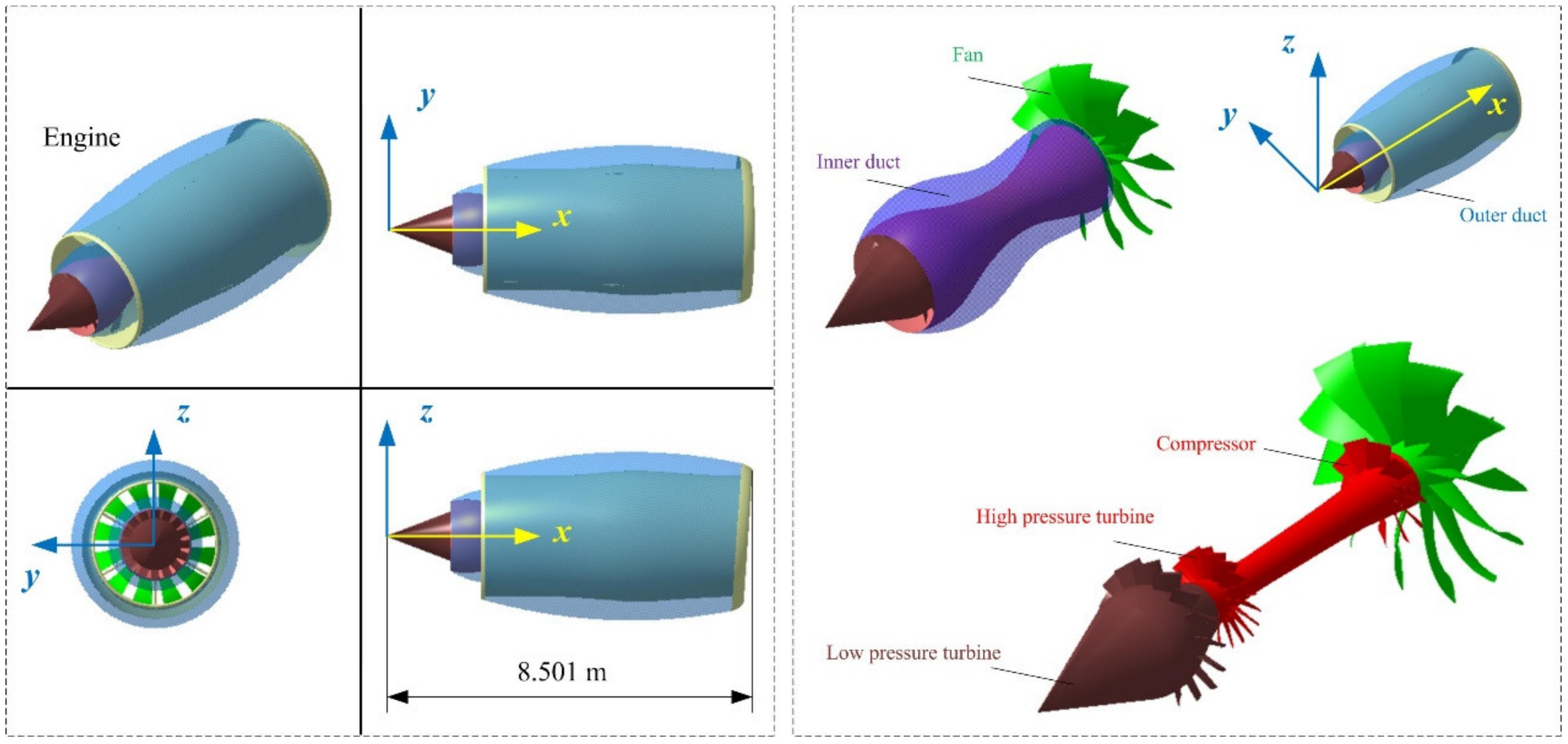
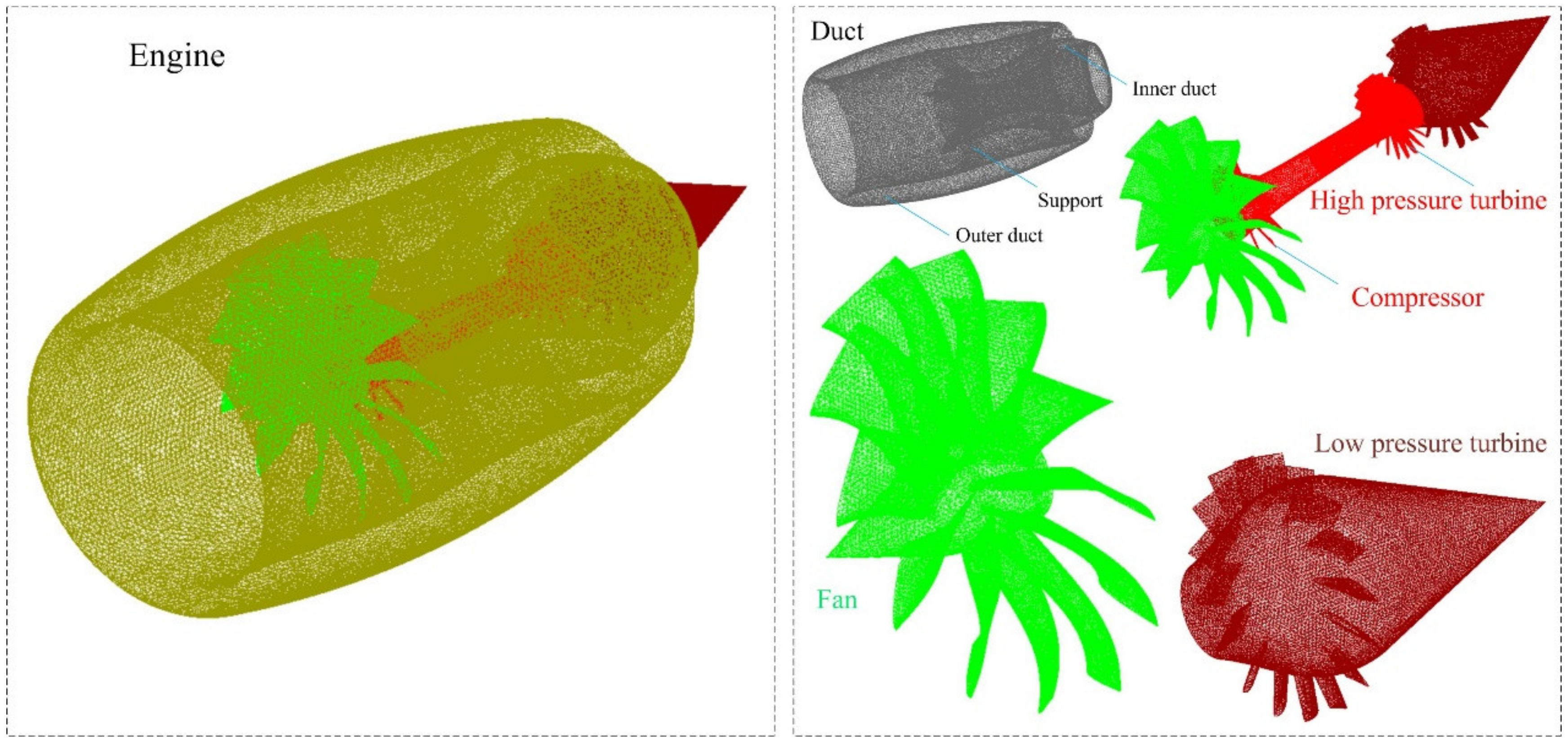
For the engine model at each observation time, the grid matrix of the whole model could be generated as follows:
M engine = M ( m fan ) ; M ( m comp ) ; M ( m h i g h ) ; M ( m l o w ) ; M ( m d u c t ) ,
where Mengine is the grid coordinate matrix of the engine model. When the rotors rotate around the x-axis, the real-time model of the fan could be updated to:
M m fan t = t r = 1 0 0 0 cos θ r , fan sin θ r , fan 0 sin θ r , fan cos θ r , fan M m fan t = 0 ,     θ r , fan = θ l t = t r .
The other rotors model could be generated as follows:
M m comp t = t r = 1 0 0 0 cos θ r , comp sin θ r , comp 0 sin θ r , comp cos θ r , comp M m comp t = 0 ,     θ r , comp = θ h t = t r
M m high t = t r = 1 0 0 0 cos θ r , high sin θ r , high 0 sin θ r , high cos θ r , high M m high t = 0 ,     θ r , high = θ h t = t r
M m low t = t r = 1 0 0 0 cos θ r , low sin θ r , low 0 sin θ r , low cos θ r , low M m low t = 0 ,     θ r , low = θ l t = t r ,
where the duct model of the engine is considered to be stationary, so its mesh matrix is not transformed.
The dynamic scattering method (DSM) is verified by PO+MOM/MLFMM (multilevel fast multipole method) in FEKO as shown in Figure 2, where fR is the radar wave frequency. The RCS-α curve determined by DSM is generally consistent with the results of FEKO, where the mean value of the DSM RCS-α curve is 1.59 dBm2 smaller than that of FEKO and there are errors in some local peaks, because different mesh types and RCS algorithms are used. The quasi-static principle (QSP) is used to discretize the high-speed rotation state of the fan at a few time sample points. The calculation results show that the DSM values in the given time range are consistent with the discrete calculation values, showing that DSM is accurate and efficient.
The above calculation results also show that the RCS of the individual fan has changed more than 21.92 dBm2 in a very short time, so it is necessary to study the dynamic electromagnetic scattering of the engine blade. More information about the RCS algorithm test is shown in Figure A1. In the following calculations, if not specified, the radar wave frequency is always 6 GHz, horizontal polarization.

3. Model

The geometric model of a turbofan engine is conceived by the full factorial design (FFD) as shown in Figure 3, where Lduct is the length of the duct, Acut is the cutting angle of the end face of the duct inlet, Rduct is the outer radius of the duct, noting that the duct includes the outer duct, the inner ducts, and the associated support components.
The geometric characteristics of the engine are shown in Table 1, where the four rotors are designed with different airfoil data, including AG 08, AG 25, AH 21, and ARA-D 10%. The outer duct of the entire engine is approximately a spiral body, because the design of Acut makes the upper end of the engine casing entrance slightly longer than the lower end. The number of blades of these rotors is different, which also leads to different base pass times.
Based on the above geometric design and related parameters, the entire engine model is built as shown in Figure 4, where the total length of the engine is 8.501 m. The engine model consists of the duct, the fan, the compressor, the high-pressure turbine, and the low-pressure turbine. The head direction of the engine points in the positive direction of the x-axis, and the central axis of rotation coincides with the x-axis.
The low-speed shaft of the turbofan engine is set to 8000 r/min and the high-speed shaft to 10,000 r/min as shown in Table 2 when the engine is working properly. The duct is set to be stationary, while the fan and the low-pressure turbine rotate around the low-speed shaft, and the compressor and the high-pressure turbine rotate around the high-speed shaft.
Fine meshing of this engine and its components is shown in Figure 5, where the duct model is composed of the outer duct, the inner duct, and associated support structures. The size data of each part when determining the high-precision mesh is shown in Table 3, where the global minimum mesh size has a maximum value of 2 mm, and local density increase technology of the grid is used where the geometric size changes dramatically, including the leading and trailing edge regions of each rotor.

4. Results and Discussion

Figure 6 supports that the electromagnetic scattering effect of the fan surface also changes in a very short time (from t = 2.083 × 10⁻⁴ s to t = 4.167 × 10⁻⁴ s). In the irradiated area of the radar wave, the upper surface of most of the blades shows a deep red color, indicating that this area is a strong source of electromagnetic scattering. The hub portion presents a lighter red color because the head has a conical design that deflects the radar wave to a nonthreatening direction. The blade root forms a certain occlusion of the joint between the hub and the blade, so a small amount of orange yellow appears here. These results show that DSM could well simulate the rotation of the blade and calculate its electromagnetic scattering characteristics.
Blade rotation is a continuous and long-term process when the turbofan engine is running normally. Therefore, the dynamic electromagnetic scattering characteristics of the various components of the engine and its entirety require a lot of calculation and analysis as shown below.

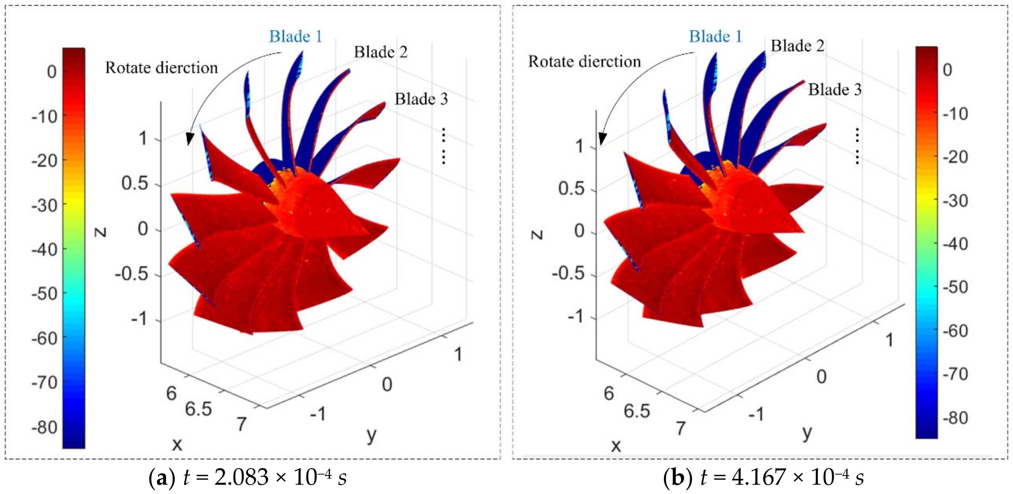
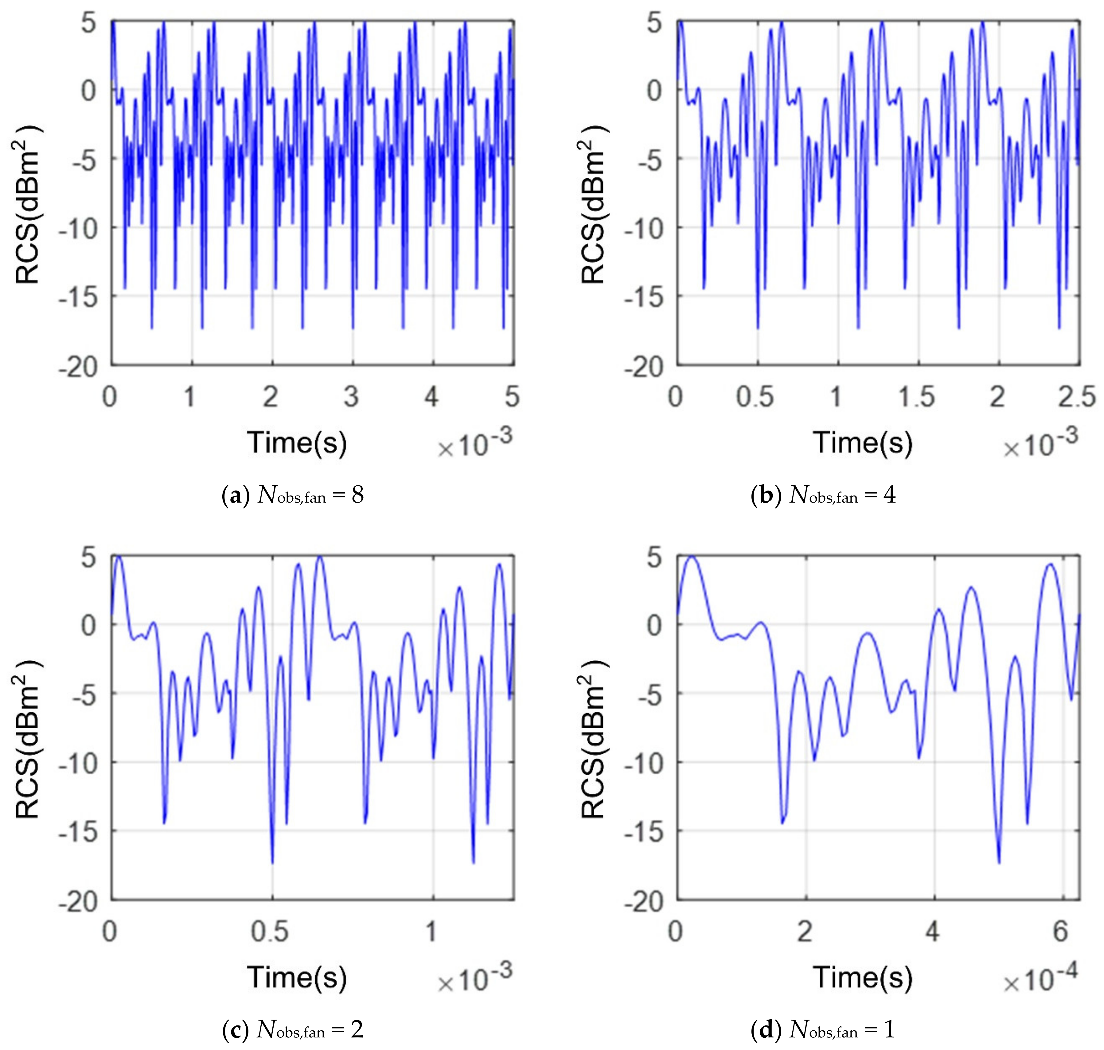
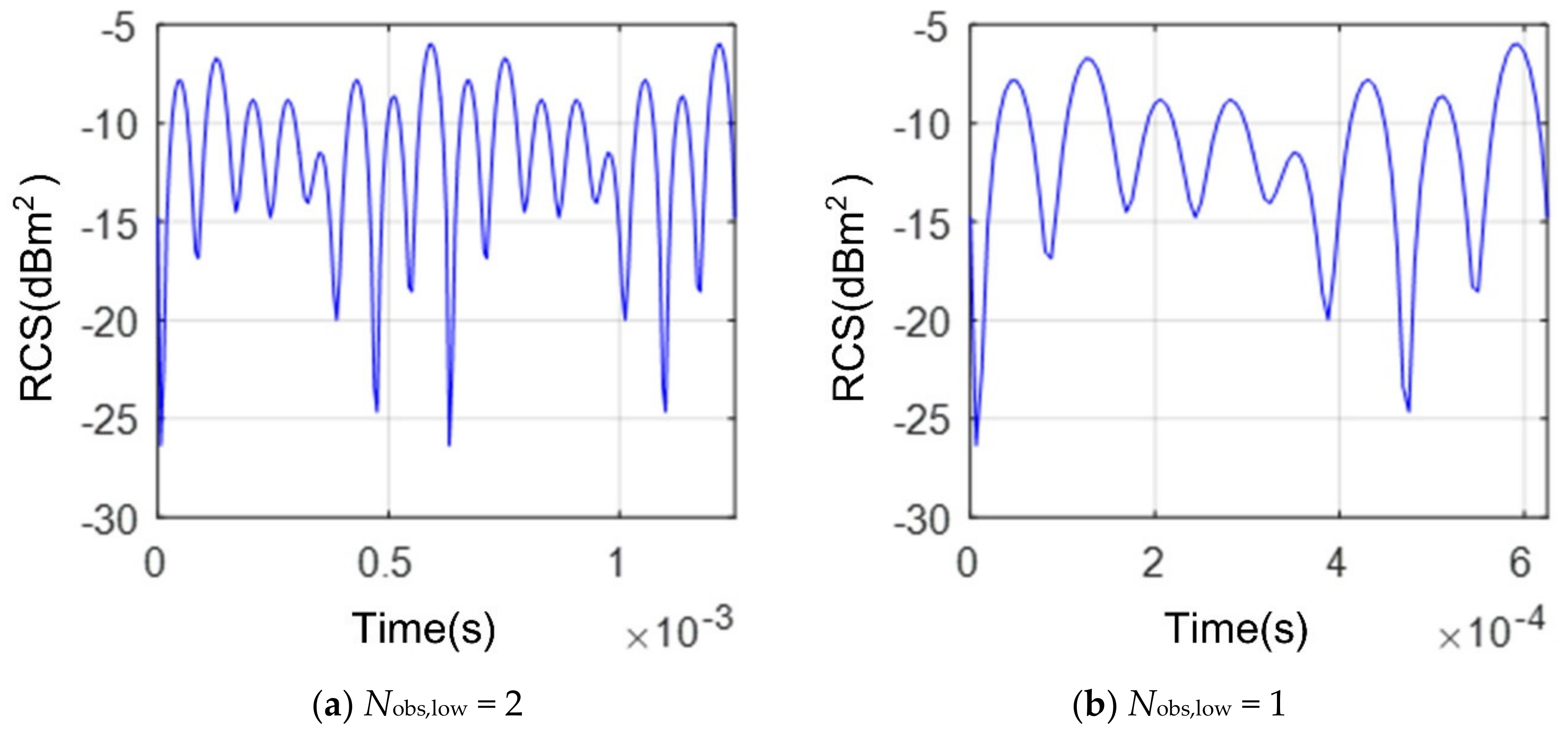
4.1. Effect of Individual Rotor

Figure 7 shows that there is an obvious periodicity in the electromagnetic scattering characteristics of the fan observed in a long time. It could be seen that the period of dynamic electromagnetic scattering of the fan is 6.25 × 10⁻³ s, which is also the basic pass time because the fan uses a uniform distribution of blade design and the rotating speed remains the same. The maximum RCS of the fan in one observation period is 4.928 dBm2 appearing at t = 1.875 × 10⁻⁵ s, while the minimum size is −17.35 dBm2 appearing at t = 5 × 10⁻⁴ s. This shows that the DSM could capture the electromagnetic scattering characteristics of the fan well for a long time, and the rotation of the fan will have a greater impact on this characteristic.
Figure 8 reveals that the electromagnetic scattering characteristics of the low-pressure turbine also exhibit periodicity within the given observation time. The dynamic RCS period of the low-speed turbine is still 6.25 × 10⁻⁴ s because the low-pressure turbine and the fan share a low-speed shaft. The minimum value of the RCS-time curve of the low-pressure turbine is −26.35 dBm2 at t = 6.25 × 10⁻⁶ s, while the maximum value is −5.983 dBm2 at t = 5.937 × 10⁻⁴ s. These results show that the observation time has a non-negligible influence on the dynamic electromagnetic scattering of the low-pressure turbine.
As the observation time increases, the RCS of the rotor on the low-speed axis of the engine changes periodically, while the degree of undulation is large, which will affect the electromagnetic scattering characteristics of the forward and tail directions of the target.

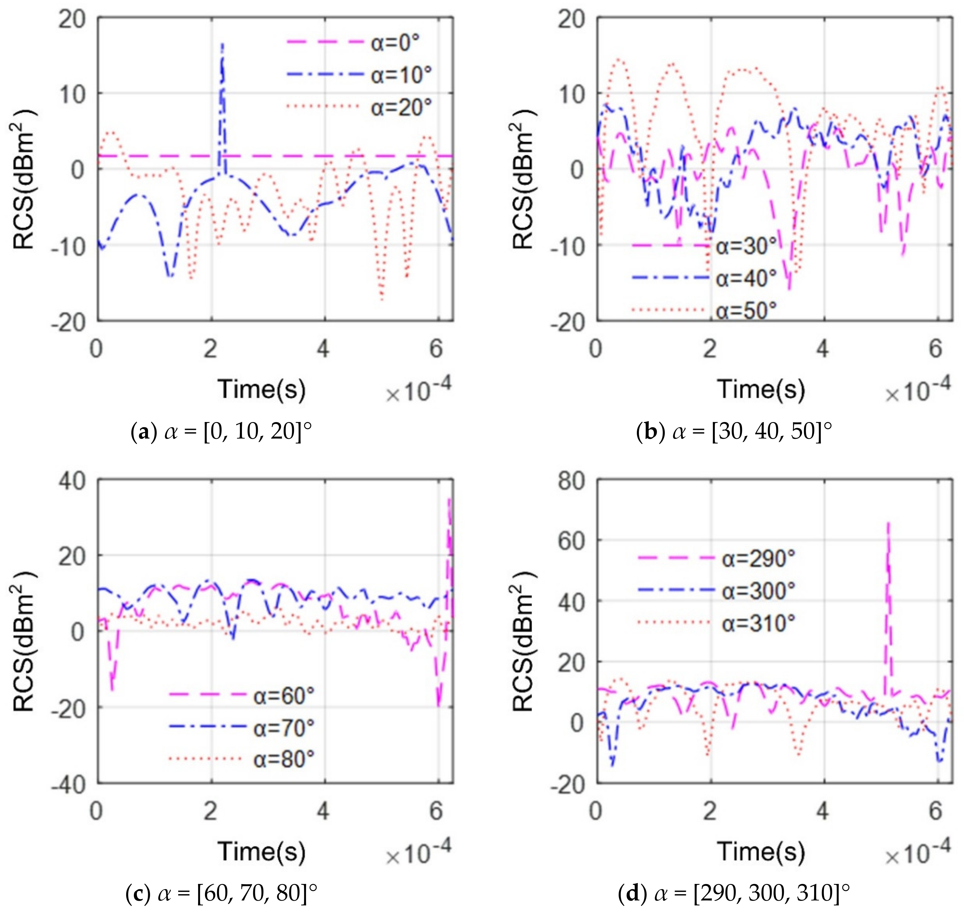
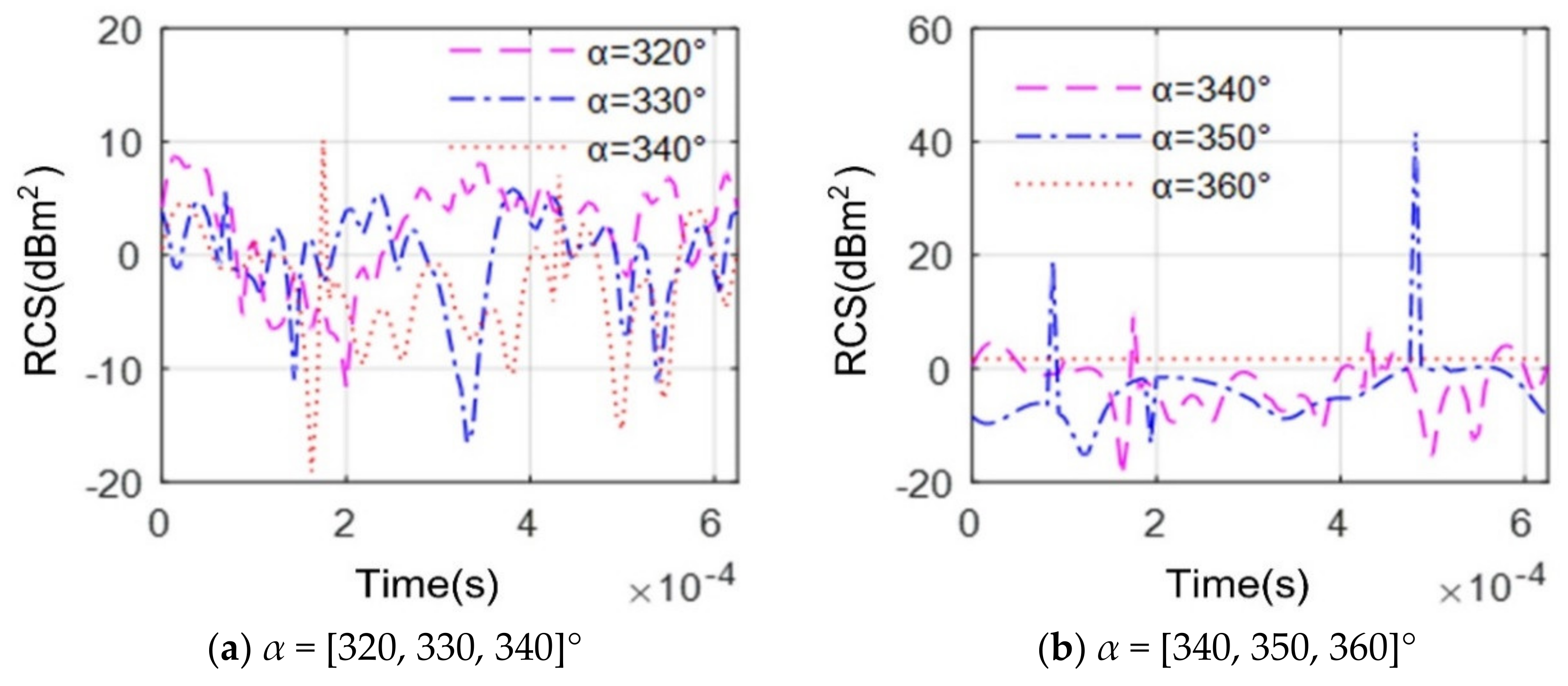
4.2. Effect of Azimuth Angle

Figure 9 indicates that the dynamic RCS of the fan at different azimuths is very different, including shape, peak, and range of variation. For the RCS-time curve with α = 0°, the RCS value is almost always maintained at 1.708 dBm2, because the fan rotating plane is perpendicular to the radar wave at this time, causing the electromagnetic scattering change caused by the rotation to be too small to be found in the current observation scale. When α = 10°, the overall change of RCS-time curve is relatively flat, but a peak of up to 17.04 dBm2 appears at t = 2.188 × 10⁻⁴ s, because the fan rotates 10.5024° at this time and the fan adopts a gradual twist and a variable chord design, this makes the roots of the blades in the upper left part and the leading edges of other blades become strong scattering sources. When α increases from 10° to 50°, the number of fluctuations of the RCS-time curve is obviously increased, and the variation law is also different, because the angle between the normal direction of the rotating surface of the fan and the radar wave is getting bigger and bigger, while the electromagnetic scattering caused by the blades and the hub is getting stronger. The two RCS-time curves of α = 70° and 80° are similar in shape, while the RCS-time curve with α = 60° shows a peak of up to 35.48 dBm2 at t = 6.188 × 10⁻⁴ s, since the fan rotates 35.48° at this time, the upper-right part of the upper surface of the blade makes the main contribution to the peak. It should also be noted that the RCS-time curve at α = 290° shows a peak with a size of 65.86 dBm2 at t = 5.125 × 10⁻⁴ s, because the incident wave is almost perpendicular to the left contour of the front of the hub at this time, the outer end faces of the left blades, the side of the hub, and the root surface of the blades in the illuminated area all have larger RCS. These results indicate that the azimuth has a significant impact on the dynamic RCS of the fan.
Figure 10 manifests that as the azimuth increases, the RCS-time curve of the fan gradually becomes stable overall within the given azimuth range. The RCS-time curve at α = 320° generally shows a wave shape that decreases first and then increases, while the peak value is 8.738 dBm2 appearing at t = 1.25 × 10⁻⁵ s. The minimum value of the RCS-time curve at α = 330° is −16.55 dBm2 but the peak value of the RCS-time curve at α = 350° is as high as 43.2 dBm2. When α increases from 320° to 360°, the angle between the normal of the rotating plane of the fan and the radar wave is decreases, which makes the strong scattering source of the fan surface gradually decrease within the same observation scale.
Table 4 presents that azimuth has a very significant effect on the RCS mean of the fan within one observation period. When α increases from −10° to 80°, the RCS mean in one observation period of the fan decreases first and then increases, where the maximum difference is 24.115 dBm2. The change in RCS within ±10° azimuths of the head indicates that the dynamic electromagnetic scattering of the fan will affect the RCS at important azimuth angles in the head direction of the engine.
Figure 11 demonstrates that the RCS-time curves of the low-pressure turbine at different azimuths vary widely, including peaks, ranges of changes, and number of fluctuations. For the RCS-time curve at α = 150°, the peak value is only −2.155 dBm2 at t = 4.594 × 10⁻⁴ s. When α is increased by 10°, the RCS-time curve changes in a similar pattern, while the RCS-time curve remains substantially straight (RCS equals 6.799 dBm2) at the current observation scale when α is increased to 180°, for the reason that the normal direction of the rotating plane of the low-pressure turbine is perpendicular to the radar wave, while the size of the hub is larger than that of the blade, which will form strong scattering and cover the RCS changes caused by the rotation of the blades. When α continues to increase to 210°, the shape of its RCS-time curve is similar to that at α = 150°, but the peak becomes −2.808 dBm2 at t = 3.281 × 10⁻⁵ s. These results show that the effect of azimuth on the low-pressure turbine is also evident.
It could be found that although the outer diameter of the low-pressure turbine is smaller than that of the fan, the RCS generated by the low-pressure turbine in the positive tail direction is larger than the RCS generated by the fan in the positive head direction.

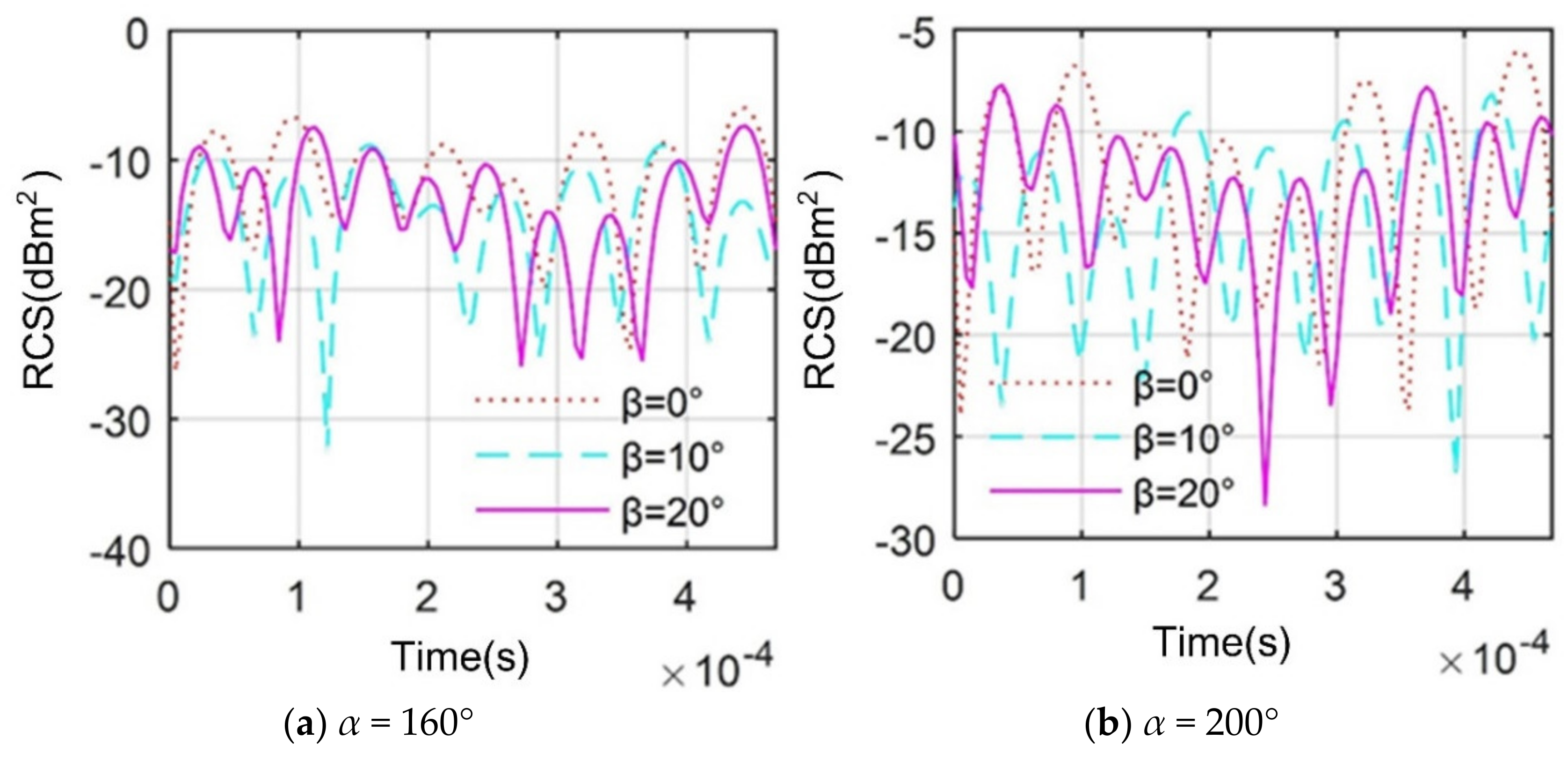
4.3. Effect of Elevation Angle

Figure 12 investigates that the dynamic RCS-time curves of low-pressure turbines at different elevation angles vary widely, including curve shape and minimum and maximum position. When α = 160°, the increase in the elevation angle will significantly increase the number of fluctuations in the RCS-time curve. For the RCS curves of α = 200°, the curves at β = 0° and 20° are similar in shape but the undulation strength is somewhat different, where the former peak is −6.064 dBm2 at t = 4.453 × 10⁻⁴ s and the latter has a peak value of −7.715 dBm2 at t = 3.750 × 10⁻⁵ s. The increase in the elevation angle directly increases the angle between the normal direction of the rotating plane of the low-pressure turbine and the radar wave, which will result in a strong scattering source on the hub and part of the blade surface. These results show that DSM could well demonstrate the effect of elevation angle change on the dynamic RCS of the low-pressure turbine and the change at this time is also not negligible.
Figure 13 presents that the effect of the elevation angle on the dynamic RCS of the low-pressure turbine is more pronounced under the current azimuths, including the aspects of minimum values, peak values, and variation laws. For the RCS-time curve at α = 150°, the increase in β significantly increases the fluctuation of the RCS curve, where the minimum values of RCS at β = 0°, 10°, and 20° are −19.16, −22.25, and −32.06 dBm2, respectively. When α = 150°, the shape of the RCS-time curve at β = 20° still appears to change too much, where the maximum value is 3.063 dBm2 at t = 1.641 × 10⁻⁴ s and the minimum value is −30.36 dBm2 at t = 9.375 × 10⁻⁶ s; the reason for the negative peak here is mainly the fact that the trailing edge of the blade in the illuminated area, the upper surface of the right blade, and the head of the propeller hub has a good effect of deflecting radar waves. These results indicate that the engine will have different stealth responses according to the elevation angle under current conditions.
Table 5 supports that an increase in the angle of the elevation will have a significant impact on the RCS mean of the low-pressure turbine at the given azimuths. When α = 150° and 210°, an increase in β will result in an increase in the RCS mean. However, when α = 160° and 200°, the increase in β will cause the RCS mean to decrease and then increase. This shows that choosing the right azimuth and elevation angle is beneficial to reduce the electromagnetic scattering intensity of the low-pressure turbine.
Overall, when approaching the positive tail direction, the RCS index of the low-pressure turbine generally decreases with the increase in β, noting that α = 180° is the positive tail direction.

4.4. Effect of Engine Duct

Figure 14 provides that the addition of engine duct greatly increases the RCS level of the combination with the fan within the given azimuth and observation time. When α = 0°, the rotation of the fan still cannot show the change of the RCS of the assembly at the current observation scale, because the radar wave at this time is perpendicular to the normal of the rotation plane of the fan, and the scattering caused by the blade is too weak. When α is gradually increased to 20°, the fluctuation of the RCS-time curve is enhanced, including the number of fluctuations and peaks. The shape of the RCS time curve is similar when α = 30° and 40°, but the latter has more minimum values. In the negative azimuth range of the head direction, the RCS-time curve at α = 320° and 340° varies in a similar range. As the azimuth angle is further restored to the head position, the angle between the radar wave and the rotation plane of the fan gradually approaches zero, which causes the RCS to remain unchanged. Therefore, it could be seen that the RCS-time curve at α = 350° changes slowly overall, except for the two peaks. The RCS of the fan and duct combination at α = 360° is maintained at 13.66 dBm2, which is much higher than the RCS level of the individual fan (1.708 dBm2), because the large casing of the duct has more sources of strong scattering, such as the duct lip with a large curvature. These results indicate that the engine’s duct is also an important source of strong scattering but not a dynamic source of scattering here.
Figure 15 implicates that the RCS curve under the omnidirectional angle of the engine is obvious and cannot be ignored, while the RCS-time curves under different heading azimuths are very different. When t = 1.875 × 10⁻⁴ s, the peak value in the omnidirectional angle of the engine is 42.62 dBm2 at α = 0°, while that of the engine at t = 3.75 × 10⁻⁴ s is 55.41 dBm2 at α = 215.8° because the trailing edges and facets of the right blades of the low-pressure turbine is not easy to deflect the incident wave at this time. The RCS peaks at α = 90° and 270° at different times appear larger and stable, which is mainly due to the mediocre design of the huge engine duct. When α increases from 0° to 20°, the dynamic RCS curve of the engine becomes more fluctuating, but the peak and RCS averages decrease, because the strong scattering source at this time is mainly reflected in the duct of the engine, the azimuth angle increases, and the strong scattering source on the lip in the illumination area is transferred to the side of the duct. These results show that the omnidirectional RCS of the engine changes dynamically with time, and the difference of dynamic electromagnetic scattering at different azimuths is obvious.
Figure 16 suggests that the engine duct has an important effect on the electromagnetic scattering of the entire engine in the current observation azimuth and time. For the engine scattering characteristics at t = 1.875 × 10⁻⁴ s, it could be found that there are more dark red areas in the lip of the inlet, and more red areas are distributed on the right side of the duct. The left side of the fan and the inner side of the left side of the duct show more orange red. When t is increased to 3.75 × 10⁻⁴ s, the light and dark areas of the engine duct surface and its color distribution hardly change, while the color distribution of the fan surface has changed slightly and the least obvious is the blade color of the tail of low-pressure turbine, because the fan, compressor, and inner and outer ducts block more radar waves, making it difficult for them to reach the low-pressure turbine at the tail. These results indicate that the rotors inside the engine will have a dynamic effect on the electromagnetic scattering of the engine while the outer casing occupies more sources of strong scattering.
Overall, the dynamic electromagnetic scattering characteristics of the engine are very obvious, and the RCS is different under different azimuth and observation time. Studying the dynamic electromagnetic scattering of the engine is of great significance to the head and tail RCS characteristics of the aircraft.

5. Conclusions

This paper establishes a dynamic scattering method to investigate the electromagnetic scattering characteristics of a biaxial multirotor turbofan engine. Through these studies, the following conclusions could be drawn:
  • The electromagnetic scattering characteristics of each rotor during steady engine operation are periodic, and the period is equal to the base pass time of the rotor at the current rotating speed;
  • The azimuth and elevation angles have a large impact on the dynamic RCS of the engine. The fan has a great influence on the change of the engine head to the RCS, while the low-pressure turbine has a greater influence on the engine tail RCS;
  • The engine duct will greatly increase the RCS level of the entire engine, but will also block the scattering of its internal components. Front and rear rotors are the main influencing factors of engine dynamic RCS.
Future research work can focus on the electromagnetic scattering characteristics of the rotor at different engine speeds, the effect of engine dynamic RCS on aircraft stealth performance, and the change of aircraft attitude on engine RCS.

Author Contributions

Conceptualization and methodology, Z.Z. and J.H.; software, validation, and formal analysis, Z.Z.; investigation and resources, Z.Z. and J.H.; writing and visualization, Z.Z.; funding acquisition, Z.Z. All authors have read and agreed to the published version of the manuscript.

Funding

This work was supported by the project funded by the China Postdoctoral Science Foundation (Grant No. BX20200035).

Acknowledgments

Thanks to Jun Huang for his guidance on this article.

Conflicts of Interest

The authors declare no conflict of interest.

Nomenclature

αthe horizontal angle between radar station-engine connection and the positive x-axis
βthe elevation angle between the radar station and the engine
θrotation angle
θbangle between adjacent blades
Ddistance between the radar and the target
celectromagnetic wave propagation speed
Vtipline speed of the blade tip
σradar cross-section
ωlangular velocity of the low-speed shaft
ωhangular velocity of the high-speed shaft
menginethe model of the engine
Menginethe grid coordinate matrix of the engine model
tbasebase pass time
Nfannumber of fan blades
εa custom difference
Tobstotal observation time
tobservation time
Subscript
fanfan
compcompressor
highhigh-pressure turbine
lowlow-pressure turbine

Appendix A

The RCS algorithm test is shown in Figure A1, where the electromagnetic scattering characteristics of the fan model are investigated under different radar wave frequencies, different numbers of grids, and different polarization modes. The RCS-α curves are generally similar at different radar wave frequencies, where RCS average increased from less than 9 to 9.805 dBm2 as fR increased from 2 to 12 GHz. When the number of grids is greater than 1.002 × 10⁵, the calculation results of RCS tend to be stable. The fewer meshes, the rougher the model displayed, the faster the calculation speed, but the larger the error. The more the grids, the more accurate the model is described, the calculation speed is reduced but the results are accurate. In order to take into account the calculation speed and grid accuracy, the number of grids and the size of the grid at this time are set as the benchmark. The RCS curves under different polarization methods are almost the same, and the difference is less than 0.051 dBm2.
Figure A1. RCS algorithm test with mfan, α = 0~360°, β = 0°, and t = 1.25 × 10⁻⁴ s.
Energies 13 05802 g0a1

References

  1. Fedele, L.; Di Vito, L.; Ramundo, F.E. Increasing Efficiency in an Aeronautical Engine through Maintenance Evaluation and Upgrades: Analysis of the Reliability and Performance Improvements under Financial Issues. Energies 2020, 13, 3059. [Google Scholar] [CrossRef]
  2. Gao, X. Numerical Study of Infrared Radiation and Electromagnetic Scattering Characteristics of Aircraft/Exhaust System. Ph.D. Thesis, Northwestern Polytechnical University, Xi’an, China, 2016. [Google Scholar]
  3. Yang, S.N.; Zhang, Z.X.; Shao, W.R.; Deng, H.W. Numerical Investigation on Electromagnetic Scattering Characteristics for Engine Cavity with Centrocone. Aeroengine 2014, 40, 48–53. [Google Scholar]
  4. York, M.A.; Hoburg, W.W.; Drela, M. Turbofan engine sizing and tradeoff analysis via signomial programming. J. Aircr. 2017, 55, 988–1003. [Google Scholar] [CrossRef] [Green Version]
  5. Lu, W.; Huang, G.; Xiang, X.; Wang, J.; Yang, Y. Thermodynamic and Aerodynamic Analysis of an Air-Driven Fan System in Low-Cost High-Bypass-Ratio Turbofan Engine. Energies 2019, 12, 1917. [Google Scholar] [CrossRef] [Green Version]
  6. Li, Y.F.; Yang, Q.Z.; Gao, X.; Wu, Z.K. Investigation on Radar Cross-Section of S-Shaped Inlets Using IPO and EEC Method. J. Propuls. Technol. 2013, 34, 577–582. [Google Scholar]
  7. Noh, Y.H.; Park, C.S.; Yook, J.G.; Choi, W.Y.; Jang, Y.H. Analysis for Contribution of Engine Inlet Structure to Monostatic RCS of Aircraft in the VHF Band. In Proceedings of the IEEE International Symposium on Antennas and Propagation & USNC/URSI National Radio Science Meeting, Boston, MA, USA, 8–13 July 2018; pp. 2335–2336. [Google Scholar]
  8. Zhou, Z.Y.; Huang, J.; Wu, N.N. Acoustic and radar integrated stealth design for ducted tail rotor based on comprehensive optimization method. Aerosp. Sci. Technol. 2019, 92, 244–257. [Google Scholar] [CrossRef]
  9. Chen, J.J.; Huang, J.W.; Xu, J.D.; Pang, C.S.; Li, J.K. Calculation of attitude angle in dynamic radar targets electromagnetic scattering. J. Proj. Rocket. Missiles Guid. 2010, 30, 183–185. [Google Scholar]
  10. Tasic, M.; Kolundzija, B.; Milosevic, T. Domain decomposition method for scattering from an aircraft with jet engine inlet cavity. In Proceedings of the International Applied Computational Electromagnetics Society Symposium (ACES), Denver, CO, USA, 25–29 March 2018; pp. 1–2. [Google Scholar]
  11. Aiello, G.; Alfonzetti, S.; Rizzo, S.A.; Salerno, N. Multi-Objective Optimization of Thin-Film Silicon Solar Cells with Metallic and Dielectric Nanoparticles. Energies 2017, 10, 53. [Google Scholar] [CrossRef] [Green Version]
  12. Yang, S.N.; Shao, W.R.; Shang, S.T.; Deng, H.W. Study on Radar Stealth Shaping for Single Expansion Ramp with Spherical 2-D Nozzle. Aeroengine 2016, 42, 55–62. [Google Scholar]
  13. Schapker, R.L. Frequency effects of electromagnetic scattering from underdense turbulent plasmas. AIAA J. 1970, 8, 1582–1590. [Google Scholar] [CrossRef]
  14. Wang, R.G.; Cheng, Y.; Chen, W. Calculation of RCS of Intake by Means of Mode Superposition. J. Air Force Eng. Univ. (Nat. Sci. Ed. ) 2004, 5, 21–25. [Google Scholar]
  15. Ling, R.T.; Smith, T.D. Scattering of acoustic and electromagnetic waves by an airfoil. AIAA J. 1989, 27, 268–273. [Google Scholar] [CrossRef]
  16. Xiao, B.; Zhang, J. Application of SBR-Calculation the RCS of an Arbitrary Shaped Open-Ended Cavity. J. Appl. Sci. 1993, 11, 328–332. [Google Scholar]
  17. Chen, Q.; Huang, J.; Pan, M.; Lu, F. A Novel Real-Time Mechanism Modeling Approach for Turbofan Engine. Energies 2019, 12, 3791. [Google Scholar] [CrossRef] [Green Version]
  18. Zhou, Z.Y.; Huang, J.; Yi, M.X. Comprehensive optimization of aerodynamic noise and radar stealth for helicopter rotor based on Pareto solution. Aerosp. Sci. Technol. 2018, 82, 607–619. [Google Scholar] [CrossRef]
  19. Qin, J.; Pan, M.; Xu, W.; Huang, J. An Output-Based Limit Protection Strategy for Turbofan Engine Propulsion Control with Output Constraints. Energies 2019, 12, 4043. [Google Scholar] [CrossRef] [Green Version]
  20. Zhou, C.H.; Qian, W.P.; Guo, Y.Q. EM Scattering Model of Dynamic Rigid Target. J. Sichuan Armed Forces 2015, 36, 138–140. [Google Scholar]
  21. Sobczak, K.; Obidowski, D.; Reorowicz, P.; Marchewka, E. Numerical Investigations of the Savonius Turbine with Deformable Blades. Energies 2020, 13, 3717. [Google Scholar] [CrossRef]
  22. Jiang, X.W.; Zhao, Q.J. Analysis and evaluation about radar target scattering characteristics of helicopter wing components. J. Aerosp. Power 2016, 31, 2691–2700. [Google Scholar]
  23. Vijayaraghavan, D.; Keith, T.G. Grid transformation and adaption techniques applied in the analysis of cavitated journal bearings. J. Tribol. 1990, 112, 52–59. [Google Scholar] [CrossRef]
  24. Song, H.Y.; Liang, L.F.; Zhou, Z.G. The complementary energy principle and generalized variational principles of quasi-static electro-magneto-thermo-elasticity. J. Harbin Eng. Univ. 2011, 32, 33–37. [Google Scholar]
  25. Eby, M.; Holloway, G. Grid transformation for incorporating the Arctic in a global ocean model. Clim. Dyn. 1994, 10, 241–247. [Google Scholar] [CrossRef]
  26. Song, H.Y.; Li, H.B.; Liang, L.F.; Zhou, Z.G. The second H-R generalized variational principles of quasi-static electro-magneto-thermo-elasticity. Struct. Environ. Eng. 2010, 37, 8–16. [Google Scholar]
  27. Zhou, Z.Y.; Huang, J. Target head direction far field radar cross section reduction based on narrow surface element method. Optik 2020, 200, 163230. [Google Scholar] [CrossRef]
  28. Chen, H.; Wang, Z.L.; Li, J.; Zhang, M.H. Launch vehicle RCS simulation and computing method based on component decomposition. J. Spacecr. TT C Technol. 2014, 33, 198–201. [Google Scholar]
  29. Tomita, H. A stretched icosahedral grid by a new grid transformation. J. Meteorol. Soc. Jpn. Ser. II 2008, 86, 107–119. [Google Scholar] [CrossRef] [Green Version]
  30. Singh, S.K.; Khanna, K.; Bose, R.; Panigrahi, B.K.; Joshi, A. Joint-transformation-based detection of false data injection attacks in smart grid. IEEE Trans. Ind. Inform. 2017, 14, 89–97. [Google Scholar] [CrossRef]
  31. Chen, B.; Tong, C.M.; Li, X.M.; Liu, K.Y. Aircraft Target Recognition Based on HRRP. J. Microw. 2017, 33, 72–77. [Google Scholar]
  32. Qi, Y.T.; Zhang, X.Y.; Lin, G.; Li, J.Z. A simulation method of aircraft dynamic RCS. Chin. J. Radio Sci. 2018, 34, 97–103. [Google Scholar]
  33. Daroukh, M.; Moreau, S.; Gourdain, N.; Boussuge, J.F.; Sensiau, C. Tonal Noise Prediction of a Modern Turbofan Engine With Large Upstream and Downstream Distortion. J. Turbomach. 2019, 141, 021010. [Google Scholar] [CrossRef] [Green Version]
  34. Lv, Z.Y.; Wei, P. Application of small scale grid tomography velocity modeling method in timedepth conversion of low-amplitude structural region. Prog. Geophys. 2020, 1, 1–9. [Google Scholar]
  35. Pan, R.; Song, Z.; Liu, B. Optimization Design and Analysis of Supersonic Tandem Rotor Blades. Energies 2020, 13, 3228. [Google Scholar] [CrossRef]
Figure 1. Schematic diagram of dynamic electromagnetic scattering of a biaxial turbofan engine.
Energies 13 05802 g001
Figure 2. Verification of the dynamic scattering method (DSM) with mfan, β = 0°, and fR = 6 GHz.
Energies 13 05802 g002
Figure 3. Geometric configuration of a turbofan engine with full factorial design (FFD).
Energies 13 05802 g003
Figure 4. Model building and detail display of the turbofan engine.
Energies 13 05802 g004
Figure 5. Surface mesh distribution of various components of the turbofan engine.
Energies 13 05802 g005
Figure 6. Surface scattering distribution of the fan, α = 0°, β = 0°, and fR = 6 GHz; RCS unit: dBm2.
Energies 13 05802 g006
Figure 7. Influence of observation time on dynamic RCS of mfan, α = 20° and β = 0°.
Energies 13 05802 g007
Figure 8. Influence of observation time on dynamic radar cross-section (RCS) of mlow, α = 160° and β = 0°.
Energies 13 05802 g008
Figure 9. Influence of azimuth on dynamic RCS of mfan, Nobs,fan = 1 and β = 0°.
Energies 13 05802 g009
Figure 10. Influence of azimuth on dynamic RCS of mfan, α = 320°~360°, Nobs,fan = 1, and β = 0°.
Energies 13 05802 g010
Figure 11. Influence of azimuth on dynamic RCS of mlow, Nobs,low = 1, α = 150°~210°, and β = 0°.
Energies 13 05802 g011
Figure 12. Influence of elevation angle on dynamic RCS of mlow, Nobs,low = 1 and β = (0, 10, 20)°.
Energies 13 05802 g012
Figure 13. Influence of elevation angle on dynamic RCS of mlow, Nobs,low = 1 and β = (0, 10, 20)°.
Energies 13 05802 g013
Figure 14. The dynamic RCS of mfan + mduct, Nobs,fan = 1, α = (0~40 and 320~360)°, and β = 0°.
Energies 13 05802 g014aEnergies 13 05802 g014b
Figure 15. The dynamic RCS of mengine, Nobs = 1 and β = 0°.
Energies 13 05802 g015
Figure 16. Surface electromagnetic scattering characteristics of mengine, α = 20° and β = 0°; RCS unit: dBm2.
Energies 13 05802 g016
Table 1. Main geometric characteristics of the turbofan engine.
Modelmfanmcompmhighmlowmduct
AirfoilAG 08AG 25AH 21ARA-D 10%
Outer radius/m1.4850.6300.5630.8061.946
Number of blades12101816
Table 2. Motion parameters of the rotors of the turbofan engine.
Modelmfanmcompmhighmlow
Rotating speed/r/min800010,00010,0008000
Table 3. Grid size for each part of the turbofan engine.
AreaMaximum Value/mmAreaMaximum Value/mm
Global minimum size2Fan blade trailing edge5
Fan blade leading edge8Fan blade25
Fan hub35Blade trailing edge of mcomp4
Blade leading edge of mcomp10Blade of mcomp25
Hub of mcomp25Blade trailing edge of mhigh5
Blade leading edge of mhigh10Blade of mhigh25
Hub of mhigh25Blade trailing edge of mlow6
Blade leading edge of mlow10Blade of mlow25
Hub of mlow30Support50
Inner duct120Outer duct150
Table 4. Influence of azimuth on radar cross-section (RCS) mean of mfan, Nobs,fan = 1, β = 0°.
α−100102030
RCS mean/dBm223.1811.709−0.039−0.9341.427
α4050607080
RCS mean/dBm23.8839.05616.2849.7482.518
Table 5. Influence of elevation angle on RCS mean of mlow, Nobs,low = 1, RCS unit: dBm2.
α150160200210
β = 0°−6.316−10.437−10.862−6.649
β = 10°−5.450−13.122−12.813−5.474
β = 20°−0.460−12.180−11.966−0.496
Publisher’s Note: MDPI stays neutral with regard to jurisdictional claims in published maps and institutional affiliations.

