Abstract
The proliferation of solar power systems could cause instability within existing power grids due to the variable nature of solar power. A well-defined statistical model is important for managing the supply-and-demand dynamics of a power system that contains a significant variable renewable energy component. It is furthermore important to consider the inherent uncertainty in the data when modeling such a complex power system. Gaussian process regression has the potential to address both of these concerns: the probabilistic modeling of solar radiation data could assist in managing the variability of solar power, as well as provide a mechanism to deal with uncertainty. In this paper, solar radiation data was obtained from the Southern African Universities Radiometric Network and used to train a Gaussian process regression model which was developed especially for this purpose. Attention was given to constructing an appropriate Gaussian process kernel. It was found that a carefully constructed kernel allowed for the successful interpolation of global horizontal irradiance data, with a root-mean-squared error of 82.2W/m. Gaps in the data, due to possible meter failure, were also bridged by the Gaussian process with a root-mean-squared error of 94.1 W/m and accompanying confidence intervals. A root-mean-squared error of 151.1 W/m was found when forecasting the global horizontal irradiance with a forecasting horizon of five days. These results, achieved in modeling solar radiation data using Gaussian process regression, could open new avenues in the development of probabilistic renewable energy management systems. Such systems could aid smart grid operators and support energy trading platforms, by allowing for better-informed decisions that incorporate the inherent uncertainty of stochastic power systems.
1. Introduction
The variability of renewable energy resources, such as solar and wind, poses a challenge to the stability of the electricity grid. One way of mitigating this challenge is to use grid-scale energy storage systems such as lithium-ion, lead-acid and redox flow batteries as well as molten salt storage [1]. Molten salt energy storage is commonly used in conjunction with concentrated solar power (CSP) plants to store heat and allow these plants to deliver energy in the evening (when the sun has set and energy demand is typically high) [2]. Pumped hydro storage is also used to store large amounts of energy and can be used when the network needs sudden support during times of peak energy consumption [3]. In recent years, hydrogen has garnered a lot of attention as a storage medium for renewable energy due to diverse production sources [4]. In such a storage system, hydrogen (preferably produced from renewable energy sources and accordingly called ‘green hydrogen’) is converted to electrical energy and water via a fuel cell [4].
An energy system containing a large component of variable renewable energy generation as well as energy storage, requires a robust energy management system to ensure that energy is dispatched when and where needed, in the most cost-effective way, while taking into account the variability of renewable energy resources such as solar and wind [5]. Such a management system could possibly gain from the probabilistic modeling and forecasting of renewable energy resource behavior. Gaussian process regression could form part of this solution by allowing energy management entities to make better-informed decisions. The Energy [R]evolution 2010 scenario, developed by Teske et al. [6], requires renewable energy generation to constitute 40% of the global primary energy supply by the year 2030 in order to reach the climate goals set out in the Paris Agreement. Furthermore, according to the European Commission’s Energy Roadmap 2050, the share of renewable energy sources in the gross final energy consumption in the EU could top 55% by the middle of the century. As of 2017 12.1% of electricity produced worldwide were from renewable sources [7]. Finding solutions to the variability problem are therefore important. According to Bumpus and Comello [8] an average annual investment in renewable energy of US$1 trillion is required until the year 2050 in order to reach the goals of the Paris Agreement. Much of the current investment in renewable energy technology is underpinned by subsidies, which cannot be taken for granted going forward [9]. An important component of a climate change mitigation strategy should therefore be energy efficiency [9]. The proliferation of energy system data, combined with improved computational power, enable better management of complex and stochastic renewable energy systems, resulting in improved energy efficiency [10]. Gaussian process regression might therefore play a role in improving the efficiency of renewable energy systems.
The success of data analysis in grid management strategies is dependant on the quality of the energy system data [11]. There is inherent uncertainty in energy system data which affects its quality [12]. It is therefore important to define the uncertainty in such a way that its impact on data quality can be mitigated. The probabilistic nature of Gaussian process models allows for uncertainty to be well-defined [13]. Finally, determining the parameters that govern an energy system that has a high sensitivity to complex exogenous parameters, such as an energy system with a significant renewable energy component, can be expensive and time-consuming. Gaussian process regression allows for the parameters to be learned by a machine without having in-depth knowledge of the underlying energy system operation. This leads to more robust predictions of energy production [14] and improved confidence in energy system models [13].
State-of-the-art forecasting techniques for power supply and demand include numerical weather prediction (NWP), autoregression (AR), moving average (MA), autoregression moving average (ARMA), Kalman filter, artificial neural network (ANN), support vector regression (SVR) and genetic algorithm [15]. An energy forecasting method for buildings using Gaussian process regression has been introduced by Prakash et al. [16]. They have shown that Gaussian process regression produces more accurate forecasts when compared to other state-of-the-art forecasting algorithms. Gaussian process quantile regression (GPQR) is proposed by Yang et al. [11] for the formulation and prediction of the power load in a smart microgrid. The prediction performance of Gaussian process regression has been quantified by Wågberg et al. [17]. Kamath et al. [18] fitted a potential energy surface for formaldehyde using both neural networks and Gaussian process regression and then compared the errors. The vibrational spectra computed from the fitted potential energy surface were also compared to a reference vibrational spectrum for formaldehyde, in order to assess the accuracy of both methods. The Gaussian process regression was done using the Python scikit learn and different kernel functions were tested [18]. The study by Kamath et al. [18] highlights some of the advantages of Gaussian process regression over neural networks. The fitting error was found to be smaller for Gaussian process regression, as given by the root-mean-squared error, while the neural network required more data to achieve a similar error. A smaller number of points on the potential energy surface is needed for quantum dynamics calculations with Gaussian processes than is the case for neural networks, while Gaussian process regression is easier to use than neural networks. Overfitting is not as much of a concern with Gaussian process regression as it is with neural networks [18]. Gaussian Processes for Machine Learning [19] provides a unified account of the application of Gaussian process models in machine learning.
Tolba et al. [20] used Online Gaussian Process Regression and Online Sparse Gaussian Process Regression to forecast global horizontal irradiance (GHI) over time horizons ranging between 30 min and 48 h. By carefully considering kernel selection, Tolba et al. [20] have furthermore compared the performance of different kernels (simple as well as compound kernels) for application in GHI data modelling. A thorough investigation into the effect of different kernels on the performance of the model was done. Tolba et al. [20] have found that quasi-quadratic kernels are particularly useful for modelling and forecasting GHI data and suggest that a periodic component should be present in a kernel for modelling the global structure of GHI data, while a random component should be used for modelling local variation due to atmospheric disturbances. This result of Tolba et al. [20] has been confirmed in the current paper.
Prediction by making use of Gaussian processes originated with Kolmogorov (1941) and Wiener (1949). It has also found use in the field of geostatistics where it was first used by the statistician and mining engineer Danie G. Krige for the valuation of new gold mines using a limited number of boreholes [21]. It was later realized that Gaussian process regression could be used for prediction within a more general, multivariate setting [19]. It is in this multidimensional framework that Gaussian process regression will be applied in this paper.
Rasmussen and Williams [19] give important insight into the relation between Gaussian process regression and artificial neural networks. Lee et al. [22] and Matthews et al. [23] studied the similarity between infinitely wide neural networks and Gaussian processes. Novak et al. [24] expanded this neural network equivalent Gaussian process for multi-layered convolution neural networks. Gaussian process regression is more convenient to handle and interpret than neural networks [19]. Furthermore, according to Rasmussen and Williams [19], a model with a finite-dimensional parameter vector (such as artificial neural networks) will not be universally consistent. This limitation is not present with non-parametric models such as Gaussian processes. Semi-parametric models, such neural networks with a dynamic set of hidden units, is an intermediate solution to the problem of universal consistency. Another factor to consider when comparing neural networks to Gaussian process regression is the occurrence of local optima when optimizing the model: with artificial neural networks local optima can occur, while this is not the case with Gaussian process regression since its posterior is convex [19].
This paper is based on a thesis titled “Evaluating the Potential of Gaussian Process Regression for Data-driven Renewable Energy Management” (the full thesis is available at http://hdl.handle.net/10019.1/107207) [25]. It was found that Gaussian process regression can successfully interpolate and predict solar radiation data, on the condition that an appropriate kernel is constructed. The application of Gaussian process regression to solar radiation data could be valuable for the successful integration of variable renewable energy resources into the grid.
2. Gaussian Process Regression
For this paper, Gaussian process regression was done by considering inference directly in function space (an equivalent way of achieving the same result would be to consider Gaussian process regression in weight-space). Imagine a function to be an infinitely long vector, with each entry representing an instance of at an input x. By considering the instances in the vector to be properties of a stochastic process, the properties of the function can be inferred by the Gaussian process based on only a finite number of points. In order to do this, the mean and covariance of a given training set are determined as functions of the position of a data point within the data set. The covariance is encoded by making use of an appropriate kernel that employs hyperparameters to describe the relationship between data points in the set. When interpolation and prediction is done, the learnt mean and covariance are used to specify a distribution of possible outputs——for a specific input, x, given the training set . This process is illustrated in Figure 1
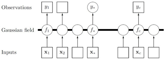
Figure 1.
Schematic illustration of Gaussian process regression [19]. to and to form the training set, while forms the test set. The Gaussian field represents the Gaussian distribution over functions.
Due to the probabilistic nature of the Gaussian process, measurement uncertainty in the training data set is well defined. However, interpolation errors could also be modelling-related. A large condition number for the covariance matrix could cause an error in the matrix computations. Scikit-learn’s GaussianProcessRegressor [26], which was used for this paper, takes care of this problem by adding value to each entry in the diagonal of the covariance matrix, thus ensuring that the matrix is positive definite.
Three kernels are of importance in this paper.
2.1. Periodic Kernel
The periodic kernel (Per) is a stationary covariance function given by
with p the period and l the characteristic length scale. The periodic kernel can be used to model functions having a repetitive pattern [27]. Figure 2 illustrates the prior and posterior of a periodic kernel and was obtained by adapting code provided by [26].
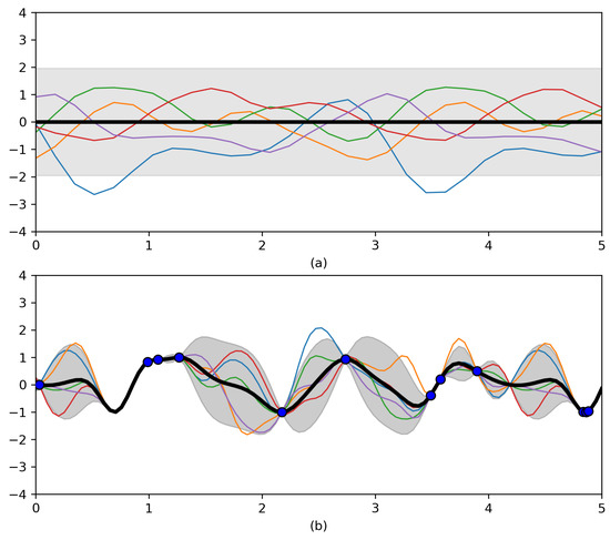
Figure 2.
(a) Five samples from a periodic kernel prior. (b) Five samples from the posterior after conditioning on twelve noise-free datapoints obtained from [26].
2.2. RBF Kernel
The radial basis function (RBF) kernel is given by
with l being the characteristic length scale, which can be tuned to specify the precise shape of the covariance function, and being a constant noise function. The RBF kernel is infinitely differentiable and is therefore handy when modeling the characteristic of smoothness of a function [26]. The RBF kernel could be used to represent a local variation within a dataset [28]. It is the most widely-used kernel [19]. Figure 3 illustrates a prior and posterior constructed by using the RBF kernel and was obtained by adapting code provided by [26].
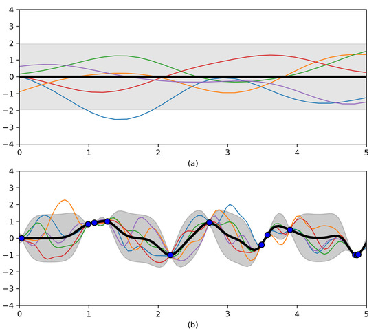
Figure 3.
(a) Five samples from a radial basis function (RBF) kernel prior. (b) Five samples from the posterior after conditioning on twelve noise-free datapoints obtained from [26].RBF kernel prior and posterior
2.3. Rational Quadratic Kernel
The rational quadratic function (RQ) is given by
where l is the characteristic length scale. The hyperparameter provides the scale mixture, which allows the rational quadratic function to act like an infinite sum of RBF kernels with different length scales. Figure 4 illustrates a prior and posterior obtained using the rational quadratic function as kernel. The figure was created by adapting code provided by [26].
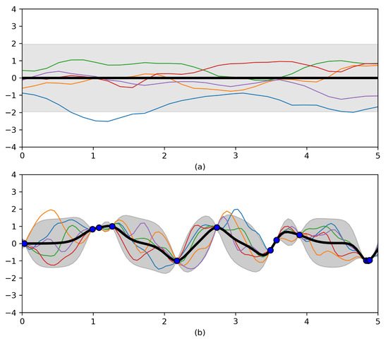
Figure 4.
(a) Five samples from a rational quadratic function prior. (b) Five samples from the posterior after conditioning on twelve noise-free datapoints obtained from [26].
3. Methodology
Weather data for the week 1 February 2015 to 8 February 2015 was acquired from the Stellenbosch weather station of the Southern African Universities Radiometric Network (Sauran) [29].
3.1. Illustrating the Possible Effect of Interval Deficiency on Weather Data
The weather data is averaged over 1 h periods for this study. This diminishes the effect of short term variability in atmospheric conditions. As Tolba et al. [20] point out, the effect of short-term variability is an important consideration when constructing a kernel. To illustrate the effect of sampling interval on data characteristics, wind speed data from the Stellenbosch weather station was sampled at different intervals, ranging from 1 h to 12 h. A Gaussian process regression was done for each of the wind speed data sets. This is illustrated in Figure 5—note how short-term variability is lost as the sampling interval increases, as well as how the confidence bounds of the Gaussian process regression become wider. For each sampling frequency, the Weibull shape and scale parameters were calculated from the Gaussian process interpolation of the wind speed and compared to reference values. The reference values for the Weibull shape and scale parameters were calculated by using wind speed data averaged every 10 min, in accordance with the IEC 61400-12-1:2005(E) standard of the International Electrotechnical Commission. The degree to which the wind speed data interpolation deviates from the real behavior of the wind resource, as the interval deficiency in the data becomes larger, is measured by the percentage deviation of the Weibull parameters from the reference values. The results are given in Table 1.
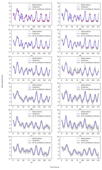
Figure 5.
Applying Gaussian process regression to interval deficient wind speed data. The wind speed data was sampled every (a) 1 h, (b) 2 h, (c) 3 h, (d) 4 h, (e) 5 h, (f) 6 h,s (g) 7 h, (h) 8 h, (i) 9 h, (j) 10 h, (k) 11 h and (l) 12 h.

Table 1.
The impact of the interval deficiency in wind speed data on the Weibull parameters, compared to wind speed data average over 10 min periods.
3.2. Gaussian Process Regression on GHI Data
Table 2 lists the weather metrics available from the Sauran Stellenbosch weather station [29]. Figure 6 includes the plots of the weather metrics, averaged over 1 h periods for the week 1 February 2015 to 8 February 2015, that were used to train the Gaussian process regression algorithm [25]. The Gaussian process algorithm will therefore use these metrics to construct a covariance matrix that represents the degree of correlation between the various weather metrics. The following metrics are expected to be strongly correlated: GHI, DNI, DHI, UVA, UVB and air temperature. The other metrics may exhibit weak correlation—whether this is the case will be determined by the Gaussian process regression algorithm. The stochastic behavior of the parameters calls for Gaussian process regression.
Table 2.
Weather metrics recorded at the Southern African Universities Radiometric Network weather station at Stellenbosch University.
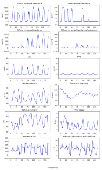
Figure 6.
Plots of the weather metrics obtained from the Stellenbosch University weather station of the South African Universities Radiometric Network, for the week 1 February 2015 to 8 February 2015.
The weather data for the week 1 February 2015 to 8 February 2015 was used to train a Gaussian process regression algorithm. A standard Gaussian process regression was employed, with a multi-in-single-out structure. This means that the Gaussian process regressor was trained on a multi-dimensional array of input data, but that interpolation and prediction was only done for a single output, namely GHI. Alternative structures for a Gaussian process regression model include online Gaussian process regression (OGPR) and online sparse Gaussian process regression (OSGPR), both of which have been investigated within the context of GHI forecasting by Tolba et al. [20].
A compound kernel, , was utilized to construct the covariance matrix. The choice of kernel was arrived at after testing different kernel configurations, such as , , and . The use of the kernel was also informed by the characteristics of the respective kernels, as described in Section 2.1, Section 2.2 and Section 2.3. The algorithm was coded in Jupyter Notebook using the Python libraries NumPy, pandas, scikit-learn and Matplotlib and is illustrated schematically in Figure 7. All code was implemented on an Intel Core i7-5600U 2.60 GHz CPU with two cores and four logical processors.
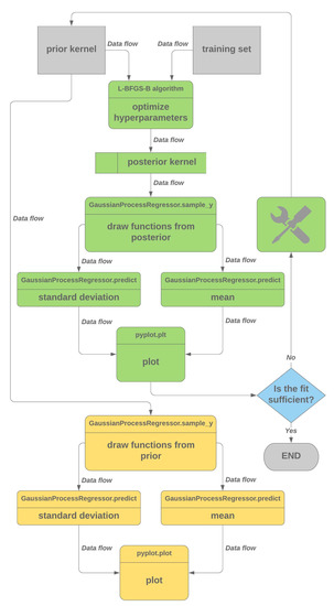
Figure 7.
Flow diagram for the implementation of Gaussian process regression that was used for this paper. Samples are drawn from the posterior after the kernel hyperparameters have been optimized based on the training set.
In order to test the ability of the algorithm to bridge gaps in the data, meter failure was simulated by removing entries within the data set from and including 2 February 2015 09:00 to 2 February 2015 16:00, as well as from and including 3 February 2015 10:00 to 3 February 2015 12:00. The resulting training data set consisted of 137 hourly data points between hours and hours. Each data point was thirteen-dimensional, [], since it contained, at each time step, readings for GHI, DNI, DHI, DHI_shadowband, UVA, UVB, air_temp, RH, WS, WD, WD_SD and BP (see Table 2).
The resulting Gaussian process model was used to interpolate global horizontal irradiance (GHI), as this parameter is generally used to calculate the available solar power at a given site on the earth’s surface. The root-mean-squared (RMS) error was used to quantify the goodness-of-fit for the interpolation. The RMS error was also employed by [20].
An attempt was also made to predict the behaviour of solar radiation data using the kernel. A Gaussian process model was trained on the data set that spanned the period from and including 1 February 2015 00:00 to 10 February 2015 05:00, while the test set comprised the rest of the GHI data up to and including 14 February 2015 23:00, concluding a two-week training and test set. No meter failure was simulated with the forecasting.
4. Results
4.1. Interpolation
Figure 8 shows the interpolation of GHI-data after training the multi-in-single-out Gaussian process regression model on the one-hourly averaged weather data set (with no meter failure), using a kernel. The inlay shows how the predictions align with measured values. The root-mean-squared error for the interpolation with meter failure, when compared to the measured GHI-values, was found to be 82.2 W/m.
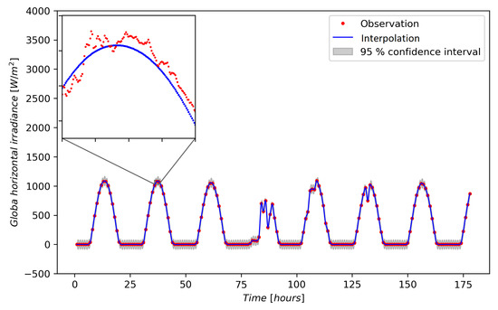
Figure 8.
Gaussian process regression of one-hourly averaged global horizontal irradiance (GHI)-data, where no meter failure is present, with a kernel. Inlay: the points constituting the Gaussian process regression, together with observations of GHI, sampled every minute.
Figure 9 shows the result of interpolating GHI-data where meter failure is present. Four different kernels were employed for this interpolation: , , and , while the Gaussian process regression model was once again trained on one-hourly averaged weather data. The root-mean-squared errors for each of the different kernels are given in Table 3.
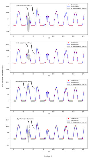
Figure 9.
Interpolation of GHI-data using different kernels, with meter failure present in the data. (a) Per, (b) quadratic function (RQ), (c) Per × RQ and (d) RBF × (RQ + Per).
Table 3.
The root-mean-square error of Gaussian process regression on one-hourly averaged data for different kernels used.
4.2. Forecasting
Figure 10 shows the result of forecasting GHI-data using the kernel. The root-mean-squared error over the forecast period was found to be 151.1 W/m.
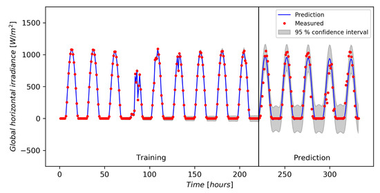
Figure 10.
Gaussian process forecast using a periodic kernel times a rational quadratic kernel.
5. Discussion
The process of interpolation of GHI data through Gaussian process regression is not trivial and clear answers on the reasons for certain kernels performing better than others are not apparent.
It was found that a compound kernel consisting of a periodic kernel component and a rational quadratic kernel component provided the best interpolation and prediction results for solar radiation data. This seems to confirm work done by Tolba et al. [5,20], who found that quasiperiodic-kernel-based GPR is particularly well-suited for modeling GHI-data. The kernel also managed to bridge gaps in the data.
Caution should be employed when interpreting the root-mean-squared error. It is used to evaluate the quality of fit of the Gaussian process regression over the whole time period and the effect of meter failure during a relatively small period of time therefore influences the root-mean-squared error disproportionately. The root-mean-squared error could, however, still be used to rank the different kernels, as was done in Table 3. The goodness-of-fit could also be evaluated by interpreting the confidence intervals on the regression points. This approach does not give an average error and allows for a localized evaluation of the goodness-of-fit. Note how the confidence intervals expand where there are gaps in the data (Figure 9).
The periodic kernel is used to model periodic structures in data, which can be transformed to quasiperiodic structures by multiplication with a non-periodic kernel [19,20]. Furthermore, the kernel incorporates different length scales, accounting for the irregular variations in the GHI-data. Tolba et al. [20] propose an interpretation for the aptness of a quasiperiodic kernel for the modelilng of GHI data: ‘The proposed interpretation is that the structure of GHI is better modelled through an omnipresent periodic component representing its global structure and a random latent component explaining rapid variations due to atmospheric disturbances.’
6. Conclusions
This paper aimed to illustrate the potential of Gaussian process regression for the interpolation and forecasting of GHI data. Reasonably good interpolation and prediction of solar radiation data were achieved by employing a multi-in-single-out Gaussian process regression with a kernel to a one-hourly averaged weather data set. The effect of sampling interval on the effectiveness of the Gaussian process regression model to capture the characteristics of a weather data set, was also briefly investigated. In this regard, it can be concluded that the sampling interval has a significant effect on the ability of the Gaussian process regression model to accurately capture the structure of a wind speed data set, as measured by the Weibull parameters. This gives rise to the question of whether a Gaussian process regression model of GHI data will be similarly affected by interval deficiency.
The reasonably successful forecasting of one-hourly averaged solar radiation data using Gaussian process regression points to the possibility of effectively integrating multi-in-single-out Gaussian process regression into a renewable energy management system. It is recommended that future work focuses on finding a rules-based method for the construction of kernels for GHI data modeling, as well as applying Gaussian process regression to larger datasets. The impact of sampling interval in Gaussian process regression models of GHI data could also make for interesting future research.
Author Contributions
Conceptualization, F.L. and J.M.; methodology, F.L. and J.M.; software, F.L.; writing—original draft preparation, F.L.; writing—review and editing, F.L., J.M. and T.H.; supervision, T.H. and J.M. All authors have read and agreed to the published version of the manuscript.
Funding
The financial assistance of the Manufacturing, Engineering and Related Services Seta (merSETA) towards this research is hereby acknowledged. Opinions expressed and conclusions arrived at are those of the authors and are not necessarily to be attributed to merSETA.
Conflicts of Interest
The authors declare no conflict of interest.
Abbreviations
The following abbreviations are used in this manuscript:
| air_temp | Air temperature |
| ANN | Artificial neural network |
| AR | Autoregression |
| ARMA | Autoregression moving average |
| BP | Barometric pressure |
| DHI | Diffuse horizontal irradiance |
| DNI | Direct normal irradiance |
| EU | European Union |
| Per | Periodic kernel |
| MA | Moving average |
| NWP | Numerical weather prediction |
| GHI | Global horizontal irradiance |
| GPQR | Gaussian process quantile regression |
| RBF | Radial basis function |
| RH | Relative humidity |
| RQ | Rational quadratic kernel |
| Sauran | Southern African Universities Radiometric Network |
| SVR | Support vector machine |
| UVA | Long-wave ultraviolet radiation |
| UVB | Short-wave ultraviolet radiation |
| WD | Wind direction |
| WD_SD | Standard deviation in wind direction |
| WS | Wind speed |
References
- Bowen, T.; Chernyakhovskiy, I.; Denholm, P. Grid-Scale Battery Storage. 2018. Available online: https://www.nrel.gov/docs/fy19osti/74426.pdf (accessed on 23 September 2020).
- Hoffmann, J.E. On the outlook for solar thermal hydrogen production in South Africa. Int. J. Hydrog. Energy 2019, 44, 629–640. [Google Scholar] [CrossRef]
- Department of Energy Republic of South Africa. Integrated Resource Plan 2018 Final Draft for Public Input. Available online: http://www.energy.gov.za/IRP/irp-update-draft-report2018/IRP-Update-2018-Draft-for-Comments.pdf (accessed on 23 September 2020).
- Sun, L.; Jin, Y.; You, F. Active disturbance rejection temperature control of open-cathode proton exchange membrane fuel cell. Appl. Energy 2020, 261, 114381. [Google Scholar] [CrossRef]
- Tolba, H.; Dkhili, N.; Nou, J.; Eynard, J.; Thil, S.; Grieu, S. GHI forecasting using Gaussian process regression. In Proceedings of the IFAC Workshop on Control of Smart Grid and Renewable Energy Systems, Jeju, Korea, 10–12 June 2019. HAL ID:hal-02051993. [Google Scholar]
- Teske, S.; Pregger, T.; Simon, S.; Naegler, T.; Graus, W.; Lins, C. Energy [r]evolution 2010—A sustainable world energy outlook. Energy Effic. 2011, 4, 409–433. [Google Scholar] [CrossRef]
- McCrone, A.; Moslener, U.; D’Estais, F.; Grüning, C.; Global Trends in Renewable Energy Investment 2018. Technical Report, FS-UNEP Collaborating Centre. 2018. Available online: http://www.iberglobal.com/files/2018/renewable_trends.pdf (accessed on 16 August 2018).
- Bumpus, A.; Comello, S. Emerging clean energy technology investment trends. Nat. Clim. Chang. 2017, 7, 382–385. [Google Scholar] [CrossRef]
- Khatib, H. IEA world energy outlook 2011—A comment. Energy Policy 2012, 48, 737–743. [Google Scholar] [CrossRef]
- Sivaram, V.; Comello, S.D.; Victor, D.G.; Sekaric, L.; Hertz-Hagel, B.; Fox-Penner, P.; Aggarwalla, R.T.; Bradbury, K.; Garg, S.; Ibrahim, E.; et al. Digital Decarbonization: Promoting Digital Innovations to Advance Clean Energy Systems; Maurice, R., Ed.; Greenberg Centre for Geoeconomic Studies: New York, NY, USA, 2018. [Google Scholar]
- Yang, Y.; Li, S.; Li, W.; Qu, M. Power load probability density forecasting using Gaussian process quantile regression. Appl. Energy 2018, 213, 499–509. [Google Scholar] [CrossRef]
- IPMVP. Concepts and options for determining energy and water savings. Int. Perform. Meas. Verif. Protoc. 2002, 1, 75–79. Available online: https://www.nrel.gov/docs/fy02osti/31505.pdf (accessed on 7 August 2018).
- Carstens, H.; Xia, X.; Yadavalli, S. Bayesian energy measurement and verification analysis. Energies 2018, 11, 380. [Google Scholar] [CrossRef]
- Burkhart, M.C.; Heo, Y.; Zavala, V.M. Measurement and verification of building systems under uncertain data: A Gaussian process modeling approach. Energy Build. 2014, 75, 189–198. [Google Scholar] [CrossRef]
- Ma, J.; Ma, X. State-of-the-art forecasting algorithms for microgrids. In Proceedings of the 2017 23rd International Conference on Automation and Computing (ICAC), Huddersfield, UK, 7–8 September 2017; pp. 1–6. [Google Scholar] [CrossRef]
- Prakash, A.K.; Xu, S.; Rajagopal, R.; Noh, H.Y. Robust building energy load forecasting using physically-based kernel models. Energies 2018, 11, 862. [Google Scholar] [CrossRef]
- Wågberg, J.; Zachariah, D.; Schön, T.B.; Stoica, P. Prediction performance after learning in Gaussian process regression. arXiv 2017, arXiv:stat.ML/1606.03865. [Google Scholar]
- Kamath, A.; Vargas-Hernández, R.A.; Krems, R.V.; Carrington, T.; Manzhos, S. Neural networks vs Gaussian process regression for representing potential energy surfaces: A comparative study of fit quality and vibrational spectrum accuracy. J. Chem. Phys. 2018, 148. [Google Scholar] [CrossRef] [PubMed]
- Rasmussen, C.E.; Williams, C.K.I. Gaussian Processes for Machine Learning; MIT Press: Cambridge, MA, USA, 2006. [Google Scholar]
- Tolba, H.; Dkhili, N.; Nou, J.; Eynard, J.; Thil, S.; Grieu, S. Multi-Horizon Forecasting of Global Horizontal Irradiance Using Online Gaussian Process Regression: A Kernel Study. Energies 2020, 13, 4184. [Google Scholar] [CrossRef]
- Minnitt, R.; Assibey-Bonsu, W.; Camisani-Calzolari, F. Keynote address: A tribute to Prof. D. G. Krige for his contributions over a period of more than half a century. Oper. Res. 2003, 405–408. Available online: http://www.saimm.co.za/Conferences/Apcom2003/405-Minnitt.pdf (accessed on 15 October 2020).
- Lee, J.; Sohl-Dickstein, J.; Pennington, J.; Novak, R.; Schoenholz, S.; Bahri, Y. Deep Neural Networks as Gaussian Processes. In Proceedings of the International Conference on Learning Representations, Vancouver, BC, Canada, 30 April–3 May 2018. [Google Scholar]
- Matthews, A.G.d.G.; Hron, J.; Rowland, M.; Turner, R.E.; Ghahramani, Z. Gaussian Process Behaviour in Wide Deep Neural Networks. In Proceedings of the International Conference on Learning Representations, Vancouver, BC, Canada, 30 April–3 May 2018. [Google Scholar]
- Novak, R.; Xiao, L.; Lee, J.; Bahri, Y.; Yang, G.; Hron, J.; Abolafia, D.A.; Pennington, J.; Sohl-Dickstein, J. Bayesian Deep Convolutional Networks with Many Channels are Gaussian Processes. arXiv 2020, arXiv:stat.ML/1810.05148. [Google Scholar]
- Lubbe, J.F. Evaluating the Potential of Gaussian Process Regression for Data-driven Renewable Energy Management. MEng (Mechanical Engineering), Stellenbosch University, South Africa. Available online: http://hdl.handle.net/10019.1/107207 (accessed on 1 October 2020).
- Pedregosa, F.; Varoquaux, G.; Gramfort, A.; Michel, V.; Thirion, B.; Grisel, O.; Blondel, M.; Prettenhofer, P.; Weiss, R.; Dubourg, V.; et al. Scikit-learn: Machine learning in Python. J. Mach. Learn. Res. 2011, 12, 2825–2830. [Google Scholar]
- Duvenaud, D.K. Automatic Model Construction with Gaussian Processes. Ph.D. Thesis, University of Cambridge, Cambridge, UK, 2014. [Google Scholar]
- Maritz, J.; Lubbe, F.; Lagrange, L. A practical guide to gaussian process regression for energy measurement and verification within the Bayesian framework. Energies 2018, 11, 935. [Google Scholar] [CrossRef]
- Brooks, M.J.; du Clou, S.; van Niekerk, J.L.; Gauche, P.; Leonard, C.; Mouzouris, M.J.; Meyer, A.J.; van der Westhuizen, N.; van Dyk, E.; Vorster, F.J. SAURAN: A new resource for solar radiometric data in Southern Africa. J. Energy S. Afr. 2015, 26, 2–10. [Google Scholar] [CrossRef]
Publisher’s Note: MDPI stays neutral with regard to jurisdictional claims in published maps and institutional affiliations. |
© 2020 by the authors. Licensee MDPI, Basel, Switzerland. This article is an open access article distributed under the terms and conditions of the Creative Commons Attribution (CC BY) license (http://creativecommons.org/licenses/by/4.0/).