Article

Multi-Horizon Forecasting of Global Horizontal Irradiance Using Online Gaussian Process Regression: A Kernel Study

1
PROMES-CNRS Laboratory (UPR 8521), Rambla de la Thermodynamique, Tecnosud, 66100 Perpignan, France
2
University of Perpignan Via Domitia, 52 avenue Paul Alduy, 66860 Perpignan, France
*
Author to whom correspondence should be addressed.
Energies 2020, 13(16), 4184; https://doi.org/10.3390/en13164184
Submission received: 17 June 2020 / Revised: 21 July 2020 / Accepted: 12 August 2020 / Published: 13 August 2020
(This article belongs to the Special Issue Solar Forecasting and the Integration of Solar Generation to the Grid)

Abstract

:
In the present paper, global horizontal irradiance (GHI) is modelled and forecasted at time horizons ranging from 30 min to 48 h , thus covering intrahour, intraday and intraweek cases, using online Gaussian process regression (OGPR) and online sparse Gaussian process regression (OSGPR). The covariance function, also known as the kernel, is a key element that deeply influences forecasting accuracy. As a consequence, a comparative study of OGPR and OSGPR models based on simple kernels or combined kernels defined as sums or products of simple kernels has been carried out. The classic persistence model is included in the comparative study. Thanks to two datasets composed of GHI measurements (45 days), we have been able to show that OGPR models based on quasiperiodic kernels outperform the persistence model as well as OGPR models based on simple kernels, including the squared exponential kernel, which is widely used for GHI forecasting. Indeed, although all OGPR models give good results when the forecast horizon is short-term, when the horizon increases, the superiority of quasiperiodic kernels becomes apparent. A simple online sparse GPR (OSGPR) approach has also been assessed. This approach gives less precise results than standard GPR, but the training computation time is decreased to a great extent. Even though the lack of data hinders the training process, the results still show the superiority of GPR models based on quasiperiodic kernels for GHI forecasting.

1. Introduction

Over the past few decades, the penetration of distributed generation in the power grid has been gaining momentum due to environmental concerns and increases in global power demand. Therefore, being able to handle an increased share of fluctuating power generation from intermittent renewable energy sources—in particular, solar photovoltaics—has become a critical challenge for power grid operators. In fact, the decentralisation of power generation has made compliance with voltage constraints, current levels and voltage drop gradients increasingly difficult and has spawned a multitude of stability, quality and safety issues. The intermittency of solar power is poorly accounted for by conventional planning strategies for the daily operation of power grids and increases the complication of voltage regulation [1]. Therefore, grid stability has become dependent upon the successful compensation of supply/demand variation. As a result, perceiving changes in the state of the power grid in real time is necessary to maintain the continuity and quality of service. Thus, smart management strategies—especially predictive management strategies—enabling the autonomous and real-time monitoring and optimisation of power grid operation are required. Predictive management strategies aggregate in situ measurements and multi-horizon forecasts—in particular, those of the grid’s load and photovoltaic power generation—in order to maintain the balance between supply and demand while ensuring grid stability at all times. Using forecasts of global horizontal irradiance (GHI), which is the total amount of shortwave radiation received from above by a surface horizontal to the ground, photovoltaic power generation can be anticipated. To this end, this paper focuses on forecasting GHI over different time horizons (i.e., from 30 min to 48 h ).
GHI is a non-stationary signal, essentially because of periodic patterns (daily and also seasonal if longer time-series are considered) arising from solar geometry and absorption and scattering in Earth’s atmosphere. Depending on how this non-stationarity is handled, two approaches can be defined. Since most classical time-series models require stationarity (or weak stationarity), a popular approach is to suppress or strongly reduce non-stationarity before modelling and forecasting the residuals. Several possibilities exist to achieve this, which are listed below.
  • Using the clearness index, defined as the ratio of irradiance at ground level to extraterrestrial irradiance on a horizontal plane (see [2,3], as well as references therein).
  • Using the clear-sky index, defined as the ratio of irradiance at ground level to clear-sky irradiance on a horizontal plane, for which a clear-sky model is needed (see [4,5], as well as references therein).
  • Fitting and then suppressing seasonal and daily patterns, without using solar geometry or radiative transfer models. Various methods can be considered, such as polynomial [6], modified gaussian [7], trigonometric [8], Fourier [9], exponential smoothing [10] or dynamic harmonic regression methods [11].
Another approach is to model and forecast raw GHI time series, without any specific preprocessing. Indeed, the transformations necessary to achieve stationarity may hinder the performance of forecasting algorithms, since the resulting time series exhibit very low correlation [12]. Incidentally, it is shown in [13] that artificial intelligence-based models using raw GHI data outperform conventional approaches based on forecasting the clearness index and are able to capture the periodic component of this time series as well as its stochastic variation. Not having to rely on clear-sky or radiative transfer models also implies that all errors come from the forecasting method itself. This is especially relevant when using clear-sky models based on mean values, as those can lead to significant errors [14].
In the last few years, GHI and photovoltaic power generation forecasting with machine learning techniques have gained in popularity. Artificial neural networks are the most commonly used tools; for further information, see the works presented in [15,16,17] or the review in [18] for a summary of existing approaches. Next are support vector machines (SVMs), which are called support vector regression (SVR) in the context of regression; more information can be found in [19] or the review in [20]. Other machine learning techniques, such as nearest neighbor, regression tree, random forest or gradient boosting, have also been tested and compared to classical time-series forecasting [21,22,23].
The use of Gaussian process regression (GPR) dedicated to GHI forecasting, however, has remained limited. In [21,23], GPR was used to obtain short-term forecasts of the clear-sky index. A more recent study has been carried out but for daily and monthly forecasting of GHI in [24]. In a spatio-temporal context, some studies based on GPR have been carried out to obtain short-term forecasts of the clear-sky index [25,26,27] (it should be noted that in these papers, the spatio-temporal covariance has been obtained by fitting empirical variograms instead of using spatio-temporal kernels). It must be stressed that, in all of these studies, in addition to forecasting the clear-sky index, no optimal kernel has been selected: as a default choice, the authors used only the square exponential kernel. In this work, GPR is used to model and forecast raw GHI data at forecast horizons ranging from 30 min to 48 h , thus covering intrahour, intraday and intraweek cases. A comparison between simple kernels and combined kernels is made, demonstrating that an appropriate choice is key to obtaining the best forecasting performance, especially at higher forecast horizons. It will be shown that, when an appropriate kernel is chosen, GPR models are sufficiently flexible to model and forecast GHI by jointly optimizing short-term variability (mainly due to atmospheric disturbances) and long-term trends (mainly due to solar geometry). As a consequence, in addition to the aforementioned benefits of not using preprocessing, the proposed models can be applied without modification in different locations, since any difference will directly be learned from the data.
The paper is organized as follows: Gaussian processes as well as commonly used covariance functions and ways of combining these functions are defined in Section 2. In Section 3, the principles of Gaussian process regression are introduced, including both online and online sparse models, as well as the estimation of their parameters and hyperparameters. The datasets used to train and validate the models included in the comparative study, derived from GHI measurements taken at the laboratory PROMES-CNRS in Perpignan (southern France), are described in Section 4. In Section 5, the forecasting accuracy of the developed OGPR and OSGPR models is evaluated. The paper ends with a conclusion. The hyperparameters’ estimated values and detailed numerical results can be found in Appendix A and Appendix B, respectively.

2. Gaussian Processes

In this section, Gaussian processes are defined. In addition, commonly used covariance functions and ways of combining these functions are presented.

2.1. Definition

A Gaussian process (GP) can be defined as a collection of random variables, any finite number of which have a joint Gaussian distribution (see Definition 2.1 in [28]). A GP defines a prior over functions, which can be converted into a posterior over functions once some data have been observed. Let us use f ( x ) G P ( μ ( x ) , k ( x , x ) ) to indicate that a random function f ( x ) follows a Gaussian process. μ ( x ) = E f ( x ) is the mean function (usually assumed to be zero), k ( x , x ) = E ( f ( x ) μ ( x ) ) ( f ( x ) μ ( x ) T ) is the covariance function and x and x are arbitrary input variables. In mathematics, GPs have been studied extensively, and their existence was first proven by the Daniell–Kolmogorov theorem (more familiar as Kolmogorov’s existence/extension/consistency theorem; see [29]). In the field of machine learning, GPs first appeared in [30], as the limiting case of Bayesian inference performed on artificial neural networks with an infinite number of hidden neurons. However, their appearance in the geostatistics research community, where they are known as kriging methods, was less recent [31,32].

2.2. Covariance Functions

A covariance function, also known as kernel, evaluates the similarity between two points and encodes the assumptions about the function to be learned. This initial belief could concern the smoothness of the function or whether the function is periodic. Any function can be used as a kernel as long as the resulting covariance matrix is positive and semi-definite. For scalar-valued inputs (x and x ), the commonly used kernels ( k WN , k SE , k RQ , k M ν and k Per ) are briefly described below. An exhaustive list of kernels can be found in [28].
  • The white noise kernel k WN is given by
    k WN ( x , x ) = σ 2 δ ( x x )
    where σ 2 is the variance. In all the considered kernels, it plays the role of a scale factor.
  • The squared exponential kernel k SE is given by
    k SE ( x , x ) = σ 2 exp ( x x ) 2 2 2
    where σ 2 is the variance and is the correlation length or characteristic length-scale, sometimes called “range” in geostatistics. controls how quickly the functions are sampled from the GP oscillate. If is large, even points that are far away have meaningful correlation; therefore, GP functions would oscillate slowly and vice versa.
  • The rational quadratic kernel k RQ is given by
    k RQ ( x , x ) = σ 2 1 + ( x x ) 2 2 α 2 α
    where σ 2 is the variance and is the correlation length. In this kernel, α defines the relative weighting of large-scale and small-scale variations. k RQ can be seen as a scale mixture of squared exponential kernels with different correlation lengths distributed according to a Beta distribution [28].
  • The Matérn class of kernels k M ν is given by
    k M ν ( x , x ) = σ 2 1 2 ν 1 Γ ( ν ) 2 ν | x x | ν B ν 2 ν | x x |
    where σ 2 is the variance, Γ is the standard Gamma function, is the correlation length and B ν is the modified Bessel function of second kind of order ν . ν controls the degree of regularity (differentiability) of the resultant GP. Kernels of the Matérn class are continuous but not differentiable. If ν = 1 / 2 , k M 1 / 2 = k E , the exponential kernel is obtained:
    k E ( x , x ) = σ 2 exp | x x |
    This kernel corresponds to the continuous version of a classical discrete autoregressive model AR(1), also known as the Ornstein–Uhlenbeck process. As discussed in [28], when ν = p 1 / 2 , with p N , the continuous version of classical AR(p) is obtained. Two other kernels of the Matérn class k M 3 / 2 and k M 5 / 2 are widely exploited in the scientific literature. These kernels correspond to the cases ν = 3 / 2 and ν = 5 / 2 , respectively. They are given by
    k M 3 / 2 ( x , x ) = σ 2 1 + 3 | x x | exp 3 | x x |
    and:
    k M 5 / 2 ( x , x ) = σ 2 1 + 5 | x x | + 5 ( x x ) 2 3 2 exp 5 | x x |
  • The periodic kernel k Per is given by
    k Per ( x , x ) = σ 2 exp 2 sin 2 π ( x x ) P 2
    where σ 2 is the variance and is the correlation length. k Per assumes a globally periodic structure (of period P) in the function to be learned. A larger P causes a slower oscillation, while a smaller P causes a faster oscillation.

2.3. Kernel Composition

Several kernels can be combined to define efficient GPs. The only thing to keep in mind is that the resulting covariance matrix must be a positive semi-definite matrix. Two ways of combining kernels while keeping the positive semi-definite property are addition and multiplication. As a result, a quasiperiodic GP can be modelled by multiplying a periodic kernel by a non periodic kernel. This gives us a way to transform a global periodic structure into a local periodic structure. For example, in [28], the product of k SE and k Per was used to model monthly average atmospheric CO 2 concentrations.
In this paper, we were inspired by [33] to construct a wide variety of kernels to model global horizontal irradiance by adding or multiplying two kernels from the kernel families presented in Section 2.2.

3. Gaussian Process Regression

In this section, standard Gaussian process regression (GPR), online Gaussian process regression (OGPR) and online sparse Gaussian process regression (OSGPR) are presented. The section ends with the training of a GPR model.

3.1. Standard Gaussian Process Regression

Consider the standard regression model with additive noise, formulated as follows:
y = f ( x ) + ε
where y is the observed value, f is the regression function, x R D × 1 is the input vector (in most cases, 1 D 3 ; in this paper, x is the time, with a dimension of 1) and ε N ( 0 , σ ε 2 ) is independent and identically distributed Gaussian noise. GPR can be defined as a Bayesian nonparametric regression which assumes a GP prior over the regression functions [28]. Basically, this consists of approximating f ( x ) GP ( μ ( x ) , k ( x , x ) ) with a training set of n observations D = { ( x i , y i ) , 1 i n } . In the following, all the input vectors x i are merged into a matrix X R n × D , and all corresponding outputs y i are merged into a vector y R n × 1 , so that the training set can be written as ( X , y ) . From Equation (9), one can see that y N μ ( X ) , K + σ ε 2 I , where K = k ( X , X ) R n × n . The joint distribution of the observed data y and the latent noise-free function on the test points f * = f ( X * ) is given in this setting by
y f * N μ ( X ) μ ( X * ) , K + σ ε 2 I K * K * T K * *
where K * = k ( X , X * ) R n × n * and K * * = k ( X * , X * ) R n * × n * .
The posterior predictive density is also Gaussian:
f * | X , y , X * N ( μ * , σ * 2 )
where:
μ * = μ ( X * ) + K * T K + σ ε 2 I 1 ( y μ ( X ) )
and:
σ * 2 = K * * K * T K + σ ε 2 I 1 K *
Let us examine what happens for a single test point x * and let k * be the vector of covariances between this test point and the n training points:
k * = [ k ( x * , x 1 ) k ( x * , x n ) ] T
Equation (12) becomes
μ * = μ ( x * ) + k * T K + σ ε 2 I 1 ( y μ ( x * ) )
Thus, μ * can be formulated as a linear combination of kernels, each one centered on a training point:
μ * = μ ( x * ) + k * T α = μ ( x * ) + i = 1 n α i k ( x i , x * )
where α = K + σ ε 2 I 1 ( y μ ( x * ) ) .
Each time a new observation is added to the observation set, the coefficients α i —referred to as parameters in the following—are updated. By contrast, the parameters of the kernel, referred to as hyperparameters, are not updated once the training is completed (see Section 3.4 and Appendix A).

3.2. Online Gaussian Process Regression

When using standard GPR, it is difficult to incorporate a new training point or a new set of training points. In case a forecasting algorithm is run in situ, there is no fixed data set D = { ( x i , y i ) , 1 i n } ; rather, one or a few observations are collected at a time and, as a result, the total amount of information available grows perpetually and incrementally. Besides, updates are often required every hour or minute, or even every second. In this case, using these methods would incur prohibitive computational overheads. Each time we wish to update our beliefs in the light of a new observation, we would be forced to invert the matrix K + σ ε 2 I with a complexity O ( n 3 ) .
A solution to this is to use online Gaussian process regression (OGPR) [34,35,36,37,38]. Let us suppose that the distribution of the GP given the first n training points ( X , y ) is known. For simplicity, let us consider μ = 0 (without loss of generality). Suppose that n + new observations are regrouped in the matrix X + ; then,
K K + + σ ε 2 I n + n + 1 = k ( X , X ) + σ ε 2 I n k ( X , X + ) k ( X + , X ) k ( X + , X + ) + σ ε 2 I n + 1
This results in the following:
K K + + σ ε 2 I n + n + 1 = K + σ ε 2 I n A K + B K + T B T K + + + σ ε 2 I n + D 1
Using the block matrix inversion theorem, we obtain
K K + + σ ε 2 I n + n + 1 = A 1 + A 1 B Δ 1 B T A 1 A 1 B Δ 1 Δ 1 B T A 1 Δ 1
where Δ = D B T A 1 B R n + × n + .
Now, inverting the ( n + n + ) × ( n + n + ) matrix only requires the inverse of A, which is known and the inversion of a n + × n + matrix. Thus, the computational cost is O ( n + 3 n 2 ) rather than O ( ( n + n + ) 3 ) when performing direct matrix inversion.

3.3. Online Sparse Gaussian Process Regression

As presented in Section 3.1, a challenge of using standard GPR is its computational complexity of O ( n 3 ) [28], within the context of training, with n being the number of training points. This principally comes from the need to invert the matrix K + σ ε 2 I in Equations (12) and (13). The simplest and most obvious approach to reducing computational complexity in Gaussian process regression is to ignore a part of the available training data: a forecast is then generated using only a subset of the available data during training, also known as the active set or inducing set. This leads to another version of OGPR: the so-called online sparse Gaussian process regression (OSGPR). OSGPR includes both the deterministic training conditional (DTC) [39] and the fully independent training conditional (FITC) [40] approximation methods. Here, computational complexity is reduced to O ( n s 2 n ) , where n s is the length of the active-set (usually n s n ). More information can be found in [38,39,40,41,42] and in the reviews presented in [34,43].
The choice of a selection procedure of the active set from the total n training points constitutes its own research field [38,39,40,41]. Sophisticated choices are based on various information criteria that quantify the pertinence of adding each point to the active-set. However, a simple way is to choose the n s points randomly—a technique known as the subset of data—which, in some situations, may be as efficient as more complex choices [44].

3.4. Training a GPR Model

As previously mentioned in the paper, there is freedom when choosing the kernel of a GPR model. The model hyperparameters, denoted as θ = θ 1 θ m T below, group those of the chosen kernel and the noise variance. As an example, the squared exponential kernel k SE (this kernel is widely used for GHI forecasting), defined by Equation (2), has two hyperparameters— σ and (see Section 2.2)—to which the noise variance σ ε 2 is added. Thus, θ = σ σ ε 2 T . The hyperparameters of all the kernels included in this comparative study are given in Appendix A (see Equations (A1)–(A16)). These hyperparameters are estimated from the data. To do so, the probability of the data given the aforesaid hyperparameters is computed. Assuming a GPR model with Gaussian noise (9), the log marginal likelihood is given by [28]
L ( θ ) = log P ( y | X , θ )
Thus,
L ( θ ) = 1 2 y T K + σ ε 2 I 1 y + log det K + σ ε 2 I + n log ( 2 π )
Usually, the estimation of θ is achieved by maximising the log marginal likelihood (21). If its gradient is known and a gradient-based algorithm, such as a conjugate gradient method, can be used (as proposed in [45]), the maximisation process may be accelerated. More information about using the gradient and Hessian of Equation (21) to speed the learning phase in the GPR algorithm can be found in [28,46,47].

4. Data Description

The data used in this comparative study originate from a rotating shadowband irradiometer (RSI), whose uncertainty range is about ± 5 % , housed at the laboratory PROMES-CNRS in Perpignan, roughly 20 k m west of the Mediterranean Sea. This device consists of two horizontally leveled silicon photodiode radiation detectors, situated in the center of a spherically curved shadowband. The region is characterised by strong winds resulting in an often clear sky, in addition to mild winters and hot and dry summers.
The comparative study enables the evaluation of GPR models through two GHI datasets, each sampled at a 30 min rate. The first one, hereafter referred to as the “summer” dataset, covers a period of 45 days, from 5 June to 18 July 2015. The second one, hereafter referred to as the “winter” dataset, also covers a period of 45 days, from 1 November to 15 December 2015.
The motivation for using two datasets instead of one larger dataset is twofold. On one hand, clear-sky days are frequent during summertime, while in winter, more complicated situations occur (overcast, broken clouds, etc.); as will be seen in the forecasting results (see Section 5.3), GHI is thus easier to predict in summer, while the winter dataset allows the highlighting of the models’ robustness in complex atmospheric conditions. On the other hand, this method allows us to show that it is not necessary to gather a huge dataset to obtain good forecasting results. If not specified otherwise, the first 30 days and the last 15 days of each GHI dataset are used for training (see Section 5.1) and to evaluate the models’ generalisation ability, respectively. Finally, the forecast horizons considered in this comparative study range from 30 min to 48 h , thus covering intrahour, intraday and intraweek cases.

5. Modeling and Forecasting Results

In this section, the modeling and forecasting results obtained using the OGPR and OSGPR models included in the comparative study as well as the evaluation metrics used are presented. The methods of initalising and estimating the hyperparameters are also explained.

5.1. Hyperparameter Initialisation and Estimation

To model GHI using Gaussian process regression, we first have to identify the most adapted kernel. In this comparative study, kernel identification is inspired by the procedure described in [33]. The main idea is to construct a wide variety of kernel structures by adding or multiplying simple kernels from the kernel families discussed in Section 2.2. While all the possible combinations of simple kernels have been evaluated, only the following kernels and combinations have been included in the comparative study.
  • Simple kernels: k E , k SE , k RQ , k M 3 / 2 , k M 5 / 2 , and k Per .
  • Quasiperiodic kernels, formulated as
    -
    products of simple kernels—i.e., k Per × E , k Per × SE , k Per × RQ , k Per × M 3 / 2 , and k Per × M 5 / 2 ;
    -
    sums of simple kernels—i.e., k Per + E , k Per + SE , k Per + RQ , k Per + M 3 / 2 , and k Per + M 5 / 2 .
As a matter of fact, results emanating from other combinations of non-periodic kernels are not presented here because they demonstrate a behaviour similar to that of simple kernels.
The maximisation of the log marginal likelihood (21) allows the estimation of kernel hyperparameters from GHI training data. Convergence to the global maximum cannot be guaranteed since L ( θ ) is non-convex with respect to θ . Several techniques can be used to remedy this issue, the most classical of which is to use multiple starting points which are randomly selected from a specific prior distribution; for instance, θ i Uniform ( 0 , 1 ) . In [48], the authors incorporate various prior types for the hyperparameters’ initial values, then examine the impact that priors have on the GPR models’ predictability. Results show that hyperparameters’ estimates, when using k SE , are indifferent to the prior distributions, as opposed to k Per , whose hyperparameters’ estimates differ along with the priors. This leads to the conclusion that prior distributions have a great influence on the hyperparameters’ estimates in the case of a periodic kernel.
As mentioned in Section 4, the two GHI datasets (i.e., the summer and winter datasets) are split into a training subset and a testing subset that cover periods of 30 days and 15 days, respectively. As for the initial values of the hyperparameters θ , we have made the following choices.
  • The correlation length has been chosen to be equal to the training data’s standard deviation.
  • In case a periodic kernel is involved in the regression process, an initial value equal to one day has been chosen for the period P in order to surpass issues that arise while estimating it.
  • The initial values of remaining hyperparameters, if any, are randomly drawn from a uniform distribution.

5.2. Evaluation of Models’ Accuracy

Two evaluation metrics are considered in this comparative study. The first one is the normalized root mean square error (nRMSE):
nRMSE = 1 n * i = 1 n * y test ( i ) y forecast ( i ) 2 1 n * i = 1 n * y test ( i )
The second evaluation metric is the correlation coefficient (R):
R = i = 1 n * y test ( i ) y ¯ test y forecast ( i ) y ¯ forecast i = 1 n * y test ( i ) y ¯ test 2 i = 1 n * y forecast ( i ) y ¯ forecast 2
where ( · ¯ is the arithmetic mean and y test R n * × 1 and y forecast R n * × 1 are the test data and forecasts given by the GPR models, respectively.
These evaluation metrics enable performance (generalisation) assessment during testing, which is a challenging task when time horizons and time scales vary, as highlighted in [21].

5.3. Forecasting Results Using OGPR

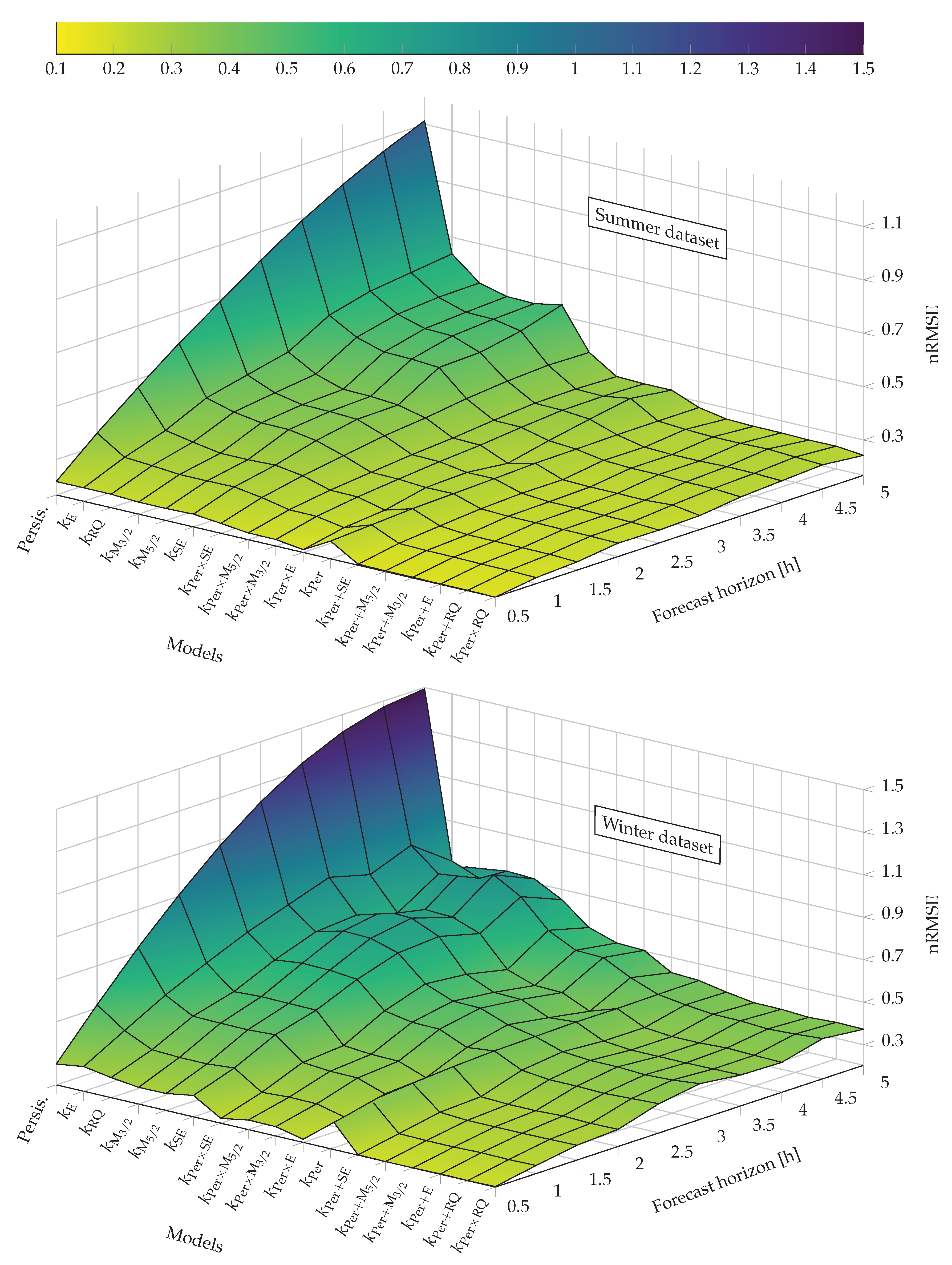
Forecasts of GHI obtained at different time horizons are compared to enable the assessment of the models’ global performance. The persistence model is used as a reference. For all the OGPR models catalogued in Section 5.1, the nRMSE vs. the forecast horizon is displayed in Figure 1. Further numerical results for the summer dataset (Table A2 and Table A3) and the winter dataset (Table A4 and Table A5) are presented in Appendix B. Broadly speaking, there are three classes of models, each possessing a different performance level. The worst performance is exhibited by the persistence model, and improved performance is witnessed when using OGPR models based on simple kernels; lastly, considerably better performance is exhibited by OGPR models based on quasiperiodic kernels, particularly considering higher forecast horizons.
For both datasets, even at the lowest forecast horizon ( 30 min ), OGPR models based on simple kernels give forecasts comparable to those given by the persistence model ( nRMSE 0.22 in summer and nRMSE 0.30 in winter), while OGPR models based on quasiperiodic kernels already give better forecasts ( nRMSE 0.18 in summer and nRMSE 0.21 in winter). As the forecast horizon increases, the persistence model’s performance degradation is more rapid than that of OGPR models. At the highest forecast horizon ( 5 h ), the persistence model gives nRMSE 1.11 in summer and nRMSE 1.50 in winter; for OGPR models based on simple kernels, nRMSE 0.55 in summer and nRMSE 0.70 in winter; for OGPR models based on quasiperiodic kernels, nRMSE 0.30 in summer and nRMSE 0.40 in winter.
Regarding OGPR models based on simple kernels, no best-performing models have been found. Depending on the forecast horizon, k M 3 / 2 , k M 5 / 2 , k SE and k RQ all alternatively give the best forecasts, while k E does not manage to perform competitively. An interesting observation is that k SE —this kernel is often used to forecast GHI; see [21,23]—does not ensure the best results among the simple kernels.
Because OGPR models based on a periodic kernel produce a periodic signal, one can say that such models are similar to clear-sky GHI models whose parameters have been fitted to the data. As a consequence, these models simply recurrently reproduce the same bell-shaped curve and produce practically the same nRMSE with respect to increasing forecast horizons. Although good forecasts can be produced by these OGPR models on clear-sky days, they are unable to predict atmospheric-disturbance-induced variability in GHI data.
However, OGPR models based on quasiperiodic kernels—these kernels combine a periodic kernel with a non-periodic kernel–possess the advantage of the periodic kernel, while still managing to predict rapid changes in GHI during the day. Among quasiperiodic kernels, k Per × RQ surpasses other kernels for the summer dataset, with k Per + M 3 / 2 , k Per + M 5 / 2 and k Per + E all coming in a close second (see Table A2); for the winter dataset, however, there is no clear best-performing kernel, as those four kernels alternatively take the first place (see Table A4).
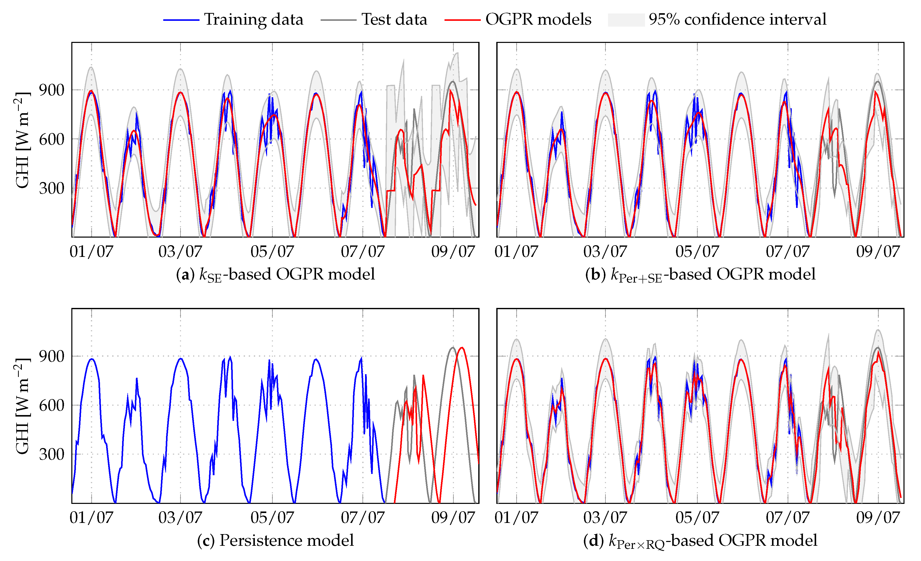
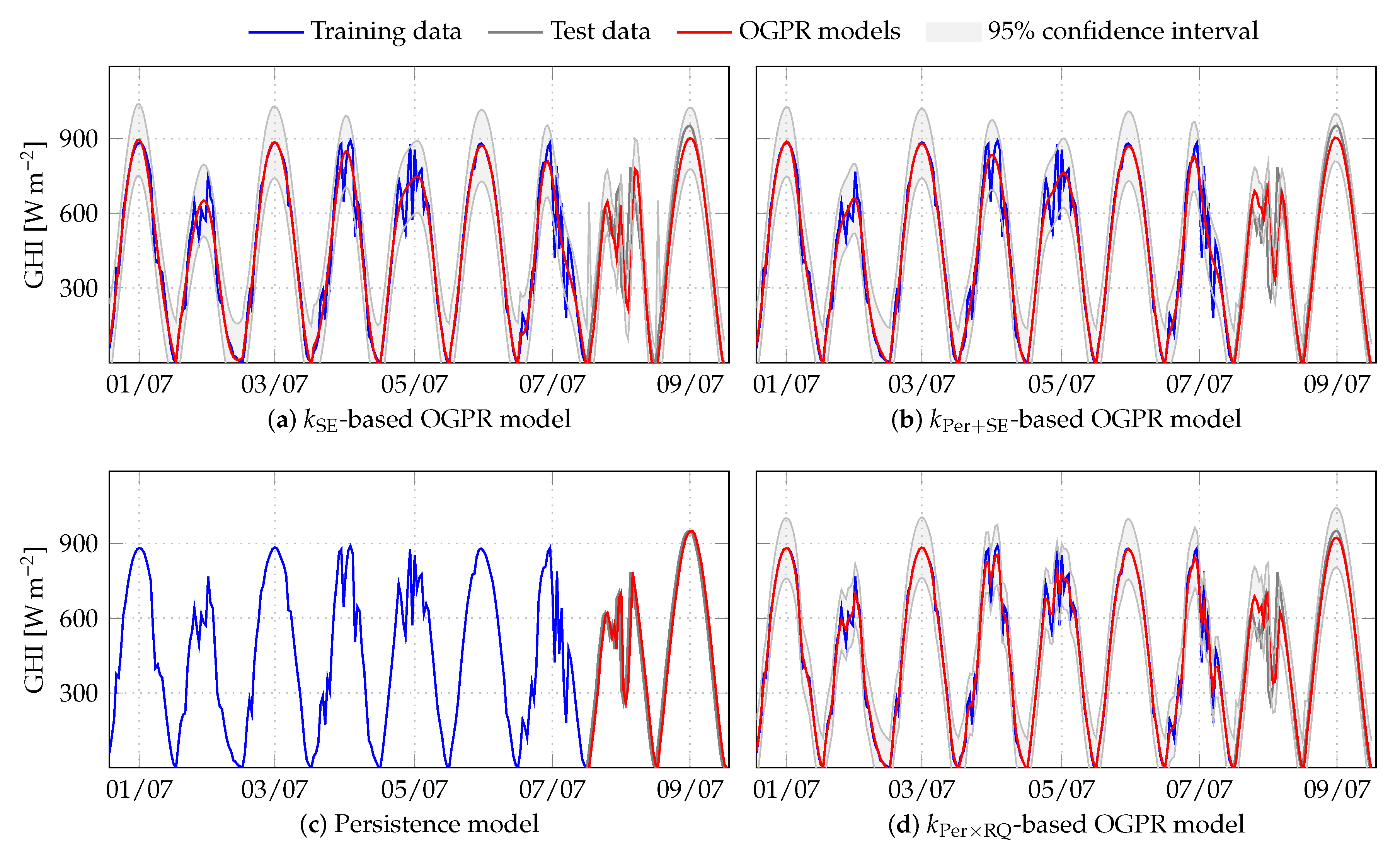
An in-depth analysis of the temporal evolution of GHI during the models’ training and testing phases sheds more light on their performance. Once more, the persistence model serves as a reference. Three OGPR models are selected: the classic k SE -based OGPR model and two of the best-performing models based on quasiperiodic kernels; i.e., the k Per × RQ -based OGPR model and the k Per + SE -based OGPR model. Here, a dataset of nine days (selected from the summer dataset) is used, split into a seven-day training subset and a two-day testing subset. In Figure 2, Figure 3 and Figure 4, 30 min , 4 h , and 48 h forecasts are shown.
Recall that, while each data sample is used during training, during testing, a new observation is added to the observation set only each whole multiple of the forecast horizon. This means that, first, for all three figures, the training results are identical; second, the coefficients α i in Equation (16) are updated every 30 min in Figure 2 and every 4 h in Figure 3, while for the 48-h forecast horizon, no update occurs.
An inspection of the seven-day training phase reveals that the data are well-fitted by every OGPR model. Signals generated by both k SE and k Per + SE are quite smooth and show few differences, as opposed to k Per × RQ , whose capability for generating more irregular signals allows it to follow the temporal evolution of GHI more closely in the case of atmospheric disturbances.
A study of the two-day testing phase reveals the following: all models perform very well when a new observation is added to the observation set every 30 min (Figure 2), although OGPR models based on quasiperiodic kernels, especially k Per × RQ , perform slightly better. The performance gap becomes more apparent when the forecast horizon increases. Thus, when a new observation is added to the observation set every 4 h , the k SE -based OGPR model struggles to predict changes in GHI accurately, as conveyed by the substantial confidence interval between observations (Figure 3a). As soon as a new observation is made, the model fits to the data, but in the absence of an update, it converges to the constant mean value learned during training (around 280 W / m 2 ). In Figure 4a, this behaviour is more obvious: no update is made throughout the entire two-day testing period, and without additional information, the OGPR model simply makes an “educated guess”, consisting of this constant mean value associated with a large confidence interval. Quasiperiodic kernels, however, do possess additional information on GHI, showing that it has a daily pattern. As with OGPR models based on simple kernels, when a new observation is added to the observation set, they fit to the data (see Figure 3b,d).
In the opposite case, OGPR models based on quasiperiodic kernels reproduce the periodic value learned during training (see Figure 4b,d), giving a result that is distinctly more faithful to the desired behaviour than a constant mean value. This explains why the performance of OGPR models based on quasiperiodic kernels degrades more slowly when the forecast horizon increases, as seen in Figure 1. Based on the results shown in Figure 3b,d, k Per × RQ is the best choice among quasiperiodic kernels as it permits sharper and more drastic changes in the modelled signal.
The nRMSE gain relative to the persistence model is presented in Table 1, for OGPR models based on the classical k SE and the three best-performing quasiperiodic kernels (winter dataset).

5.4. Forecasting Results Using OSGPR

The impact of training data sparsity on forecasting accuracy (generalisation) is assessed in this section of the paper. The subset of data technique is used; this technique simply consists of ignoring a part of the data available for training. Lowering the quantity of data used to train the models reduces computation time during training and also during testing, since the number of parameters is reduced (see Equation (16)). In addition, this allows us to evaluate the models’ ability to handle missing data in the training sequence (i.e., their generalisation ability in the case of missing data in that sequence).
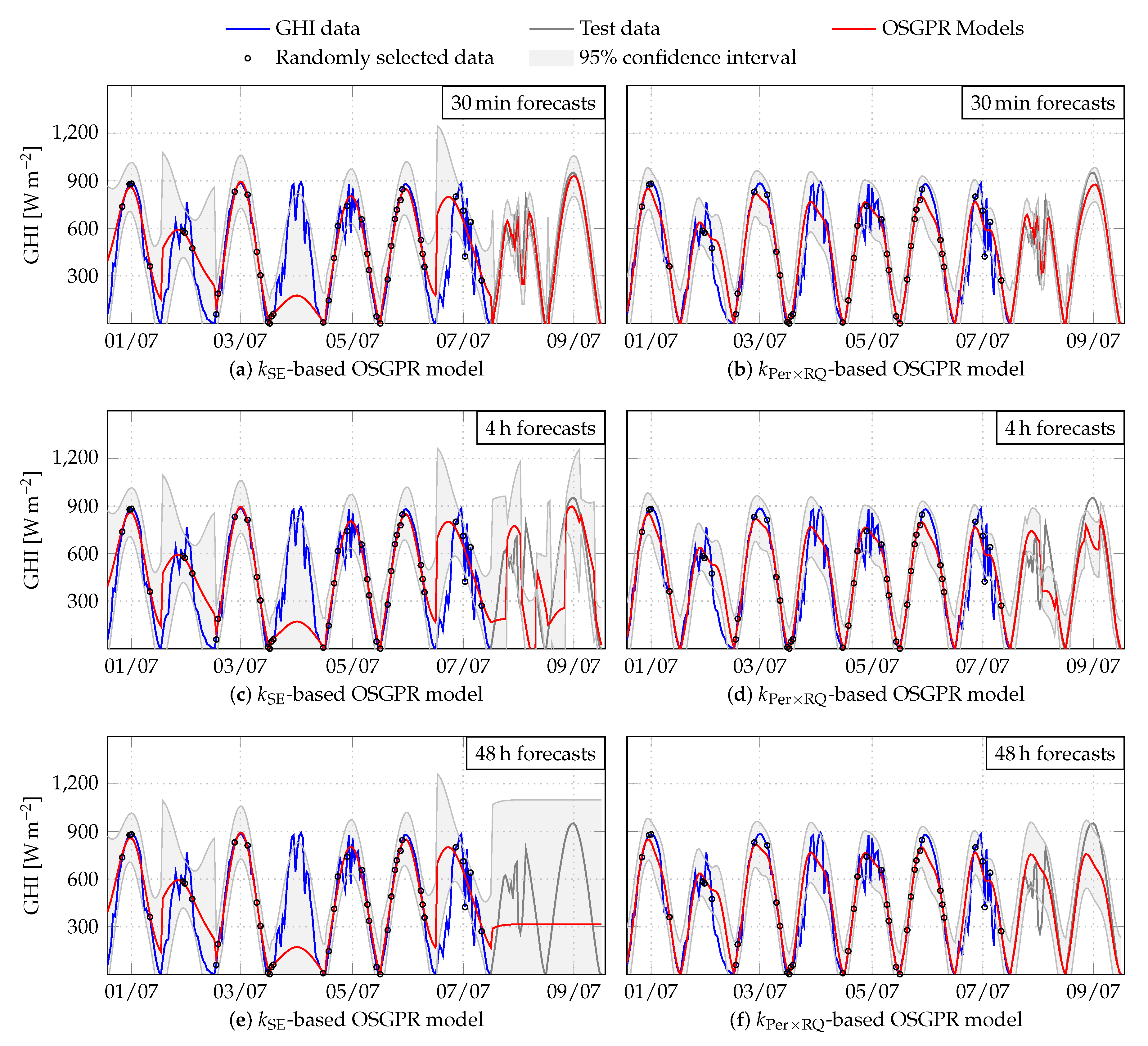
Thirty minute, 4 h and 48 h forecasts given by both the k SE -based OSGPR model and the k Per × RQ -based OSGPR model are displayed in Figure 5. The dataset constitutes the same measurements of GHI (nine days) that were considered with OGPR models (see Section 5.3). Here, however, only 20% of the available data—randomly selected from the summer dataset—have been used during training.
With this low number of training points, the OSGPR model based on k SE does not provide acceptable results. Compare, for example, the third and fourth days of training: when given sufficient data, a good fit is obtained, but if the only training points are at the beginning and the end of the day (as during the fourth day), the OSGPR model based on k SE simply makes the best inference, which, in this case, is not sufficient. In contrast, the OSGPR model based on k Per × RQ still manages to give an acceptable fit. The key here is that even a low number of training points is enough for the models based on quasiperiodic kernels to learn the daily periodic behavior of GHI.
As expected, the forecast results are good when considering the 30 min horizon, with an advantage shown for the k SE -based OSGPR model. However, as for OGPR models, when the forecast horizon increases, the superiority of the quasiperiodic kernel is shown again. It should be noted that, with a low number of data, periodic behaviour is not learned as well as before: compare Figure 5f, where the two testing days are not bell-shaped but rather resemble the last four training days, to Figure 4d). Nonetheless, this example demonstrates the usefulness of Gaussian process regression models, even in the case of (severely) missing data.
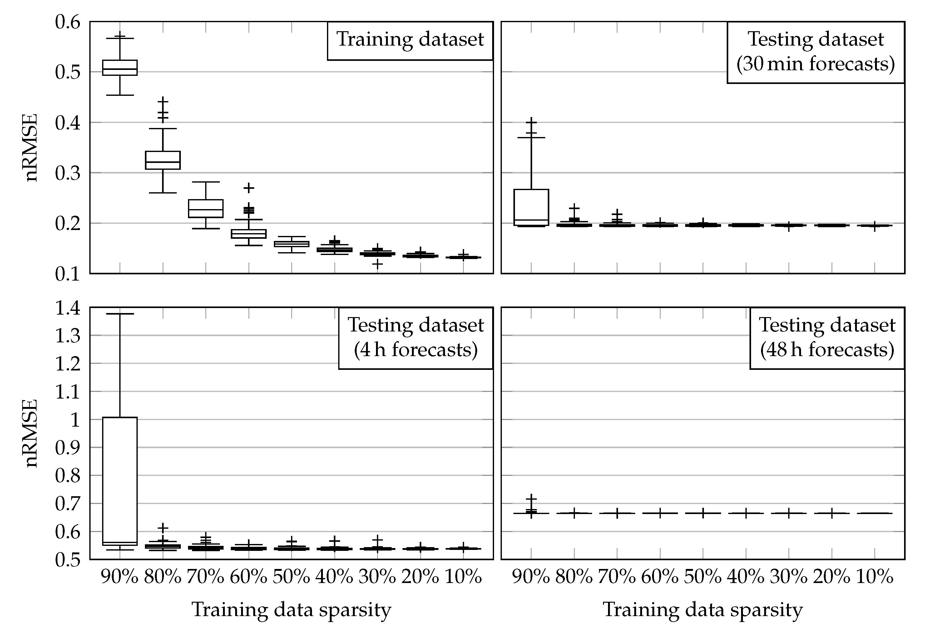
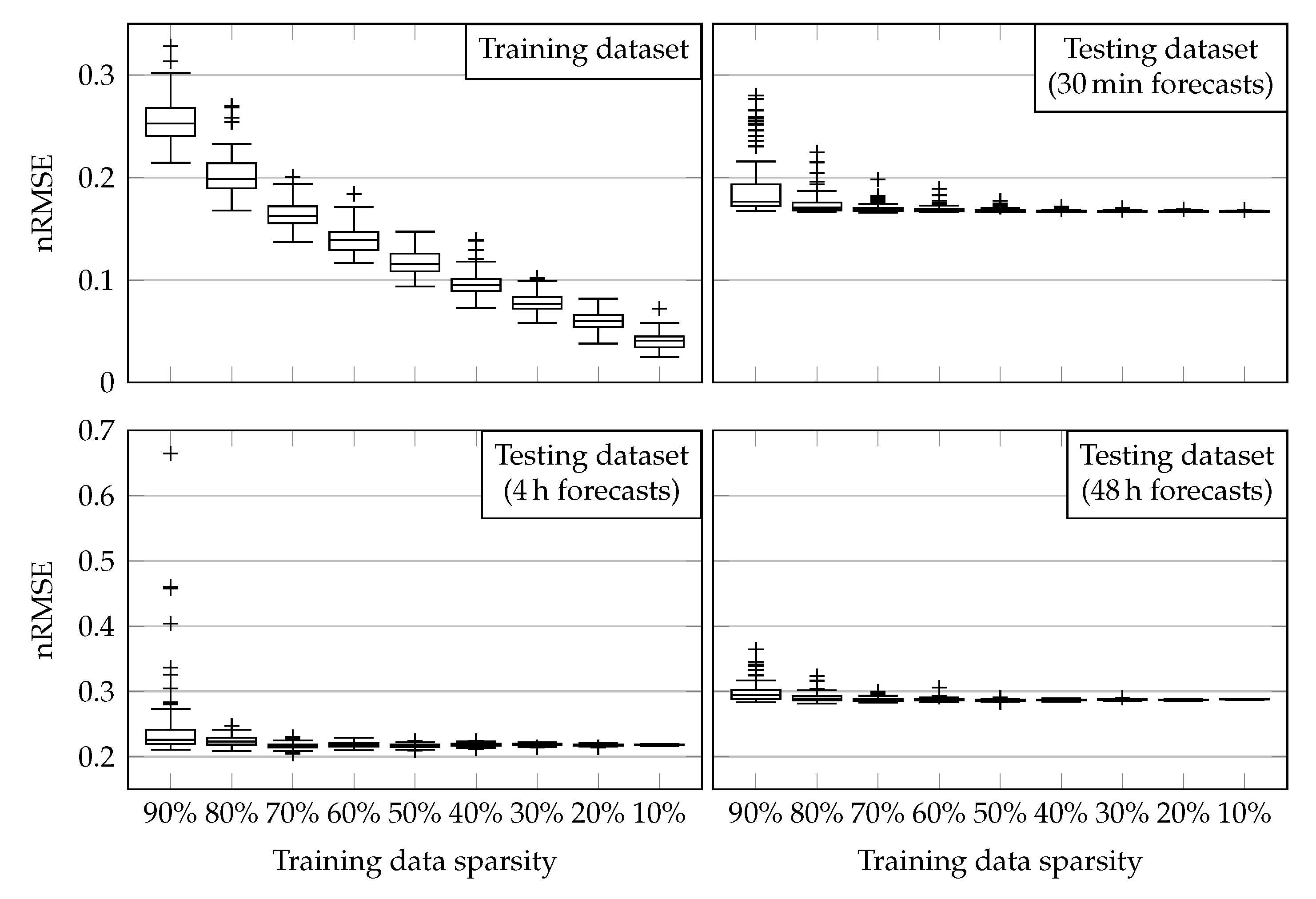
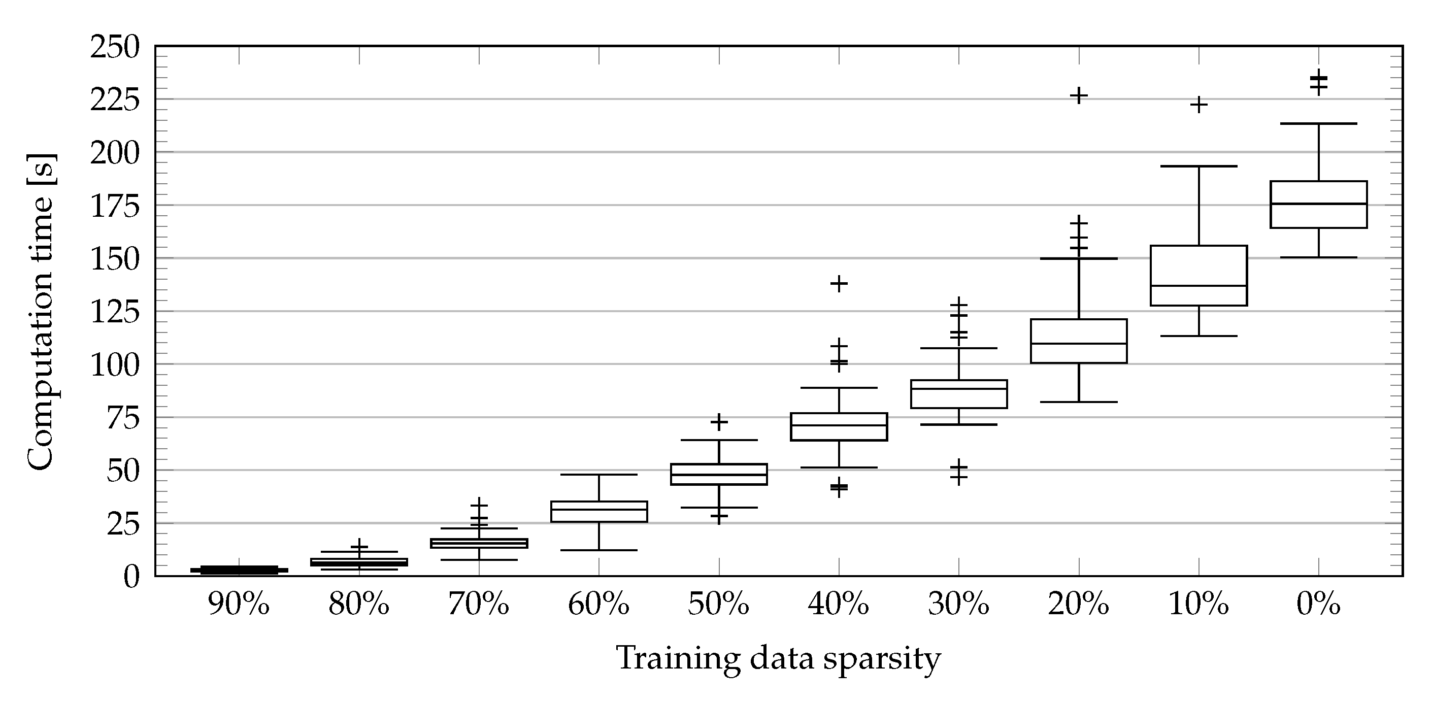
Figure 6 and Figure 7 show nRMSE vs. training data sparsity for the k SE -based OSGPR model and the k Per × RQ -based OSGPR model, respectively. Figure 8 shows the computation time vs. training data sparsity for the latter model. To avoid making conclusions based on a particular realisation (keep in mind that training data are randomly selected), 100 Monte Carlo runs have been conducted; thus, the use of box plots (the Tukey box plots display the median, 0.25-quartile and 0.75-quartile, and whiskers corresponding to ±1.5 times the interquartile range) in Figure 6, Figure 7 and Figure 8. As can be seen, if during training, nRMSE decreases steadily with data sparsity, during testing, it quickly reaches a threshold level, and dispersion also quickly vanishes. In this study, this threshold seems to be around 70%. As a consequence, using only 30% of the available training data appears to be sufficient to achieve the same nRMSE results to those obtained when using the whole training dataset. The gain in computation time is significant, as it falls from a median of 175 s at a sparsity level of 0% to a median of 17 s at a sparsity level of 70%, which amounts to around a 90% reduction.
6. Conclusions

The present paper aimed to design a Gaussian process regression model in the service of GHI forecasting at various time horizons (intrahour, intraday and intraweek). In existing research, only the squared exponential kernel k SE was used as the default choice (see [21,23]); no due attention was paid to the kernel selection and the ensuing impact of the model’s performance, which was thoroughly investigated and proven to be pertinent in this paper. A comparative study was carried out on several GPR models, ranging from rather simple models to more complex versions, such as quasiperiodic kernels that are the sum or product of a simple kernel and a periodic kernel. Two separate 45-day datasets have been used. The conclusions which arise are that GPR models predictably outperform the persistence model, and that quasiperiodic-kernel-based GPR models are particularly apt to model and forecast GHI. In the case of low forecast horizons, all OGPR models perform satisfactorily. The case of higher forecast horizons, however, is an entirely different matter, as quasiperiodic kernels prove themselves to be much more suitable for the application at hand. The proposed interpretation is that the structure of GHI is better modelled through an omnipresent periodic component representing its global structure and a random latent component explaining rapid variations due to atmospheric disturbances. The periodic component in the proposed quasiperiodic kernels opens the door to GHI forecasting at higher forecast horizons (several hours to a few days) by minimising performance degradation. Accurate GHI forecasting from intrahour to intraweek horizons thus becomes a real possibility, provided that the proper kernel is fashioned.
A simple sparse GPR approach, the subset of data technique, has also been assessed; this consists of using only a part of the available data for training. This approach gives less precise results than standard GPR, but the training computation time is decreased to a great extent: this study indicates that comparable performance (in terms of nRMSE) is obtained when using only 30% of the available training data, which leads to a 90% decrease of computation time. Additionally, even though the lack of data hinders the training process, the results still show the superiority of GPR models based on quasiperiodic kernels.
Future work will focus on some of the best-performing quasiperiodic kernels that have been put forward in this paper and assess their performance using larger GHI datasets.

Author Contributions

All authors contributed equally to this work. All authors have read and agreed to the published version of the manuscript.

Funding

This research (project Smart Occitania) was funded by the French Environment and Energy Management Agency (ADEME).

Acknowledgments

The authors would like to thank ADEME for its financial support. The authors also thank all the Smart Occitania consortium members—in particular, ENEDIS, the French distribution system operator—for their contribution to this work.

Conflicts of Interest

The authors declare no conflict of interest.

Abbreviations

The following abbreviations are used in this manuscript:
GHIGlobal horizontal irradiance
GPGaussian process
GPRGaussian process regression
OGPROnline Gaussian process regression
OSGPROnline sparse Gaussian process regression
nRMSENormalized root mean square error

Appendix A. Kernel Hyperparameters

In this appendix, the mathematical expression of the simple and quasiperiodic kernels considered in Section 5 are given. One can also find in Table A1 the estimated values of the model hyperparameters for all OGPR models, using both summer and winter datasets. As stated in Section 3.4, these hyperparameters are denoted as θ = θ 1 θ m T .
Table A1. Estimated hyperparameters of all the OGPR models included in the comparative study for both summer and winter datasets.
Kernel θ ^ 1 sum./win. θ ^ 2 sum./win. θ ^ 3 sum./win. θ ^ 4 sum./win. θ ^ 5 sum./win. θ ^ 6 sum./win.
k E 342.3/175.60.510/0.290–/––/––/––/–
k M 3 / 2 354.1/202.20.169/0.160–/––/––/––/–
k M 5 / 2 355.0/199.50.186/0.170–/––/––/––/–
k SE 351.0/168.60.140/0.080–/––/––/––/–
k Per 420.6/172.20.998/1.0001.627/0.767–/––/––/–
k RQ 348.7/176.60.110/0.0890.664/4.507–/––/––/–
k Per × E 3027.7/201.00.999/1.0016.279/0.71784.22/4.127–/––/–
k Per × M 3 / 2 270.1/157.00.972/1.0190.600/0.5131.664/1.283–/––/–
k Per × M 5 / 2 271.1/157.30.971/1.0200.599/0.5121.801/1.405–/––/–
k Per × SE 271.0/154.20.950/1.0000.570/0.5240.884/0.810–/––/–
k Per × RQ 349.9/252.60.998/1.0001.210/0.8890.065/0.2260.016/0.016–/–
k Per + E 374.3/173.10.998/1.0001.497/0.693146.2/86.760.136/0.176–/–
k Per + M 3 / 2 430.2/153.50.998/1.0001.600/0.635137.4/85.020.071/0.112–/–
k Per + M 5 / 2 371.7/151.20.998/1.0001.455/0.629137.5/85.010.079/0.123–/–
k Per + SE 355.1/153.90.998/1.0001.410/0.609128.4/81.390.060/0.070–/–
k Per + RQ 385.9/153.60.999/1.0001.494/0.643154.9/84.680.038/0.0740.170/0.736
  • Simple kernels:
    k SE ( x , x ) = θ 1 2 exp ( x x ) 2 2 θ 2 2
    k RQ ( x , x ) = θ 1 2 1 + ( x x ) 2 2 θ 3 θ 2 2 θ 3
    k E ( x , x ) = θ 1 2 exp | x x | θ 2
    k M 3 / 2 ( x , x ) = θ 1 2 1 + 3 | x x | θ 2 exp 3 | x x | θ 2
    k M 5 / 2 ( x , x ) = θ 1 2 1 + 5 | x x | θ 2 + 5 ( x x ) 2 3 θ 2 2 exp 5 | x x | θ 2
    k Per ( x , x ) = θ 1 2 exp 2 sin 2 π ( x x ) θ 2 θ 3 2
  • Products of simple kernels:
    k Per × SE ( x , x ) = θ 1 2 exp 2 sin 2 π ( x x ) θ 2 θ 3 2 ( x x ) 2 2 θ 4 2
    k Per × E ( x , x ) = θ 1 2 exp 2 sin 2 π ( x x ) θ 2 θ 3 2 | x x | θ 4
    k Per × M 3 / 2 ( x , x ) = θ 1 2 exp 2 sin 2 π ( x x ) θ 2 θ 3 2 3 | x x | θ 4 1 + 3 | x x | θ 4
    k Per × M 5 / 2 ( x , x ) = θ 1 2 exp 2 sin 2 π ( x x ) θ 2 θ 3 2 5 | x x | θ 4 · 1 + 5 | x x | θ 4 + 5 ( x x ) 2 3 θ 4 2
    k Per × RQ ( x , x ) = θ 1 2 exp 2 sin 2 π ( x x ) θ 2 θ 3 2 1 + ( x x ) 2 2 θ 5 θ 4 2 θ 5
  • Sums of simple kernels:
    k Per + SE ( x , x ) = θ 1 2 exp 2 sin 2 π ( x x ) θ 2 θ 3 2 + θ 4 2 exp ( x x ) 2 2 θ 5 2
    k Per + E ( x , x ) = θ 1 2 exp 2 sin 2 π ( x x ) θ 2 θ 3 2 + θ 4 2 exp | x x | θ 5
    k Per + M 3 / 2 ( x , x ) = θ 1 2 exp 2 sin 2 π ( x x ) θ 2 θ 3 2 + θ 4 2 1 + 3 | x x | θ 5 exp 3 | x x | θ 5
    k Per + M 5 / 2 ( x , x ) = θ 1 2 exp 2 sin 2 π ( x x ) θ 2 θ 3 2 + θ 4 2 1 + 5 | x x | θ 5 + 5 ( x x ) 2 3 θ 5 2 exp 5 | x x | θ 5
    k Per + RQ ( x , x ) = θ 1 2 exp 2 sin 2 π ( x x ) θ 2 θ 3 2 + θ 4 2 1 + ( x x ) 2 2 θ 6 θ 5 2 θ 6

Appendix B. Detailed Numerical Results

In this appendix, detailed numerical results are presented. The values of nRMSE and the correlation coefficient R can be found in Table A2 and Table A3 for the summer dataset and in Table A4 and Table A5 for the winter dataset.
Table A2. Numerical values of nRMSE obtained when performing forecasts with persistence and OGPR models (summer dataset). The forecast horizon ranges between 30 min and 5 h . The best results are highlighted in green.
Forecast Horizon30 min1 h2 h3 h4 h5 h
Persistence0.21770.34850.58330.79350.97491.1130
k E 0.21830.28180.40280.47370.59980.6382
k M 3 / 2 0.21250.26520.35740.38150.50750.5263
k M 5 / 2 0.21260.26510.35580.37920.50420.5235
k RQ 0.21790.27430.37390.41440.53770.5532
k SE 0.21530.26660.33870.37070.46600.5427
k Per 0.23400.24410.25960.27200.27720.2779
k Per + E 0.16890.19310.22090.22920.25380.2518
k Per + M 3 / 2 0.17030.19540.22230.23080.25080.2548
k Per + M 5 / 2 0.17050.19560.22260.23120.25100.2553
k Per + RQ 0.16920.19290.22000.23550.25260.2529
k Per + SE 0.17140.19860.22680.23450.25480.2588
k Per × E 0.17790.20980.25850.24800.31180.3192
k Per × M 3 / 2 0.19220.22800.26600.29200.32110.3188
k Per × M 5 / 2 0.19270.22890.26770.29470.32370.3220
k Per × RQ 0.16750.18990.21760.21970.24840.2424
k Per × SE 0.20450.25060.30610.34620.38250.3886
Table A3. Numerical values of the correlation coefficient R obtained when performing forecasts with persistence and OGPR models (summer dataset). The forecast horizon ranges between 30 min and 5 h . The best results are highlighted in green.
Forecast Horizon30 min1 h2 h3 h4 h5 h
Persistence0.94620.86180.61190.2835−0.0773−0.3992
k E 0.94450.90570.79730.70290.50520.4196
k M 3 / 2 0.94680.91400.83560.82820.63920.5999
k M 5 / 2 0.94680.91430.83750.83000.64480.6058
k RQ 0.94480.90960.82110.79140.58930.5528
k SE 0.94680.91650.86190.82680.71650.6108
k Per 0.94780.93610.92300.91340.90910.9085
k Per + E 0.96730.95740.94390.94130.92540.9259
k Per + M 3 / 2 0.96490.95310.93960.93900.92690.9222
k Per + M 5 / 2 0.96490.95300.93940.93880.92680.9220
k Per + RQ 0.96570.95640.94350.93760.92680.9240
k Per + SE 0.96570.95300.93720.93680.92300.9202
k Per × E 0.96400.94910.92180.92810.88370.8807
k Per × M 3 / 2 0.95850.94070.91580.90790.87980.8807
k Per × M 5 / 2 0.95830.94010.91470.90610.87760.8781
k Per × RQ 0.96770.95840.94500.94510.92780.9311
k Per × SE 0.95250.92740.88560.86880.82240.8201
Table A4. Numerical values of nRMSE obtained when performing forecasts with persistence and OGPR models (winter dataset). The forecast horizon ranges between 30 min and 5 h . The best results are highlighted in green.
Forecast Horizon30 min1 h2 h3 h4 h5 h
Persistence0.30090.51670.90621.21681.41821.4934
k E 0.31930.42500.61540.76220.77650.7128
k M 3 / 2 0.27650.35420.51300.70860.65890.7448
k M 5 / 2 0.27760.35420.51120.70490.65350.7383
k RQ 0.29470.36330.51190.67760.61650.6793
k SE 0.30120.36820.51630.66920.61180.6676
k Per 0.34790.36620.39880.41290.41710.4218
k Per + E 0.20440.24100.28640.35910.35170.3729
k Per + M 3 / 2 0.20280.23880.28100.37040.34460.3839
k Per + M 5 / 2 0.20280.23890.28100.37100.34470.3848
k Per + RQ 0.20320.23990.28150.36780.34660.3817
k Per + SE 0.20420.24210.28730.38130.35750.4043
k Per × E 0.21660.26080.31800.45330.37140.4408
k Per × M 3 / 2 0.24340.28960.36320.49770.42640.5138
k Per × M 5 / 2 0.24450.29090.36510.50000.42940.5186
k Per × RQ 0.20540.24220.28330.38190.34200.3801
k Per × SE 0.22560.28470.37760.54040.48000.5505
Table A5. Numerical values of the correlation coefficient R obtained when performing forecasts with persistence and OGPR models (winter dataset). The forecast horizon ranges between 30 min and 5 h . The best results are highlighted in green.
Forecast Horizon30 min1 h2 h3 h4 h5 h
Persistence0.92990.79320.3666−0.1357−0.5436−0.7250
k E 0.91080.84940.65790.45910.39580.5041
k M 3 / 2 0.93970.89990.77610.57700.59690.5018
k M 5 / 2 0.93920.89980.77740.57960.60290.5071
k RQ 0.93060.89280.77240.58460.64260.5557
k SE 0.92730.88930.76720.58610.64990.5666
k Per 0.91470.89440.86870.85830.85550.8522
k Per + E 0.96750.95470.93540.89990.90350.8880
k Per + M 3 / 2 0.96780.95540.93750.89280.90670.8809
k Per + M 5 / 2 0.96780.95530.93750.89240.90670.8803
k Per + RQ 0.96770.95500.93730.89450.90590.8825
k Per + SE 0.96730.95390.93430.88510.89890.8678
k Per × E 0.96310.94610.91860.83150.88710.8371
k Per × M 3 / 2 0.95320.93300.89490.78710.85250.7696
k Per × M 5 / 2 0.95280.93240.89360.78490.85010.7647
k Per × RQ 0.96710.95390.93620.88460.90680.8825
k Per × SE 0.95990.93540.88400.74560.80350.7334

References

  1. Dkhili, N.; Eynard, J.; Thil, S.; Grieu, S. A survey of modelling and smart management tools for power grids with prolific distributed generation. Sustain. Energy Grids Netw. 2020, 21, 100284. [Google Scholar] [CrossRef]
  2. Lorenz, E.; Heinemann, D. Prediction of Solar Irradiance and Photovoltaic Power. In Comprehensive Renewable Energy; Sayigh, A., Ed.; Elsevier: Amsterdam, The Netherlands, 2012; pp. 239–292. [Google Scholar]
  3. Inman, R.H.; Pedro, H.T.; Coimbra, C.F. Solar forecasting methods for renewable energy integration. Prog. Energy Combust. Sci. 2013, 39, 535–576. [Google Scholar] [CrossRef]
  4. Ineichen, P. Comparison of eight clear sky broadband models against 16 independent data banks. Sol. Energy 2006, 80, 468–478. [Google Scholar] [CrossRef] [Green Version]
  5. Nou, J.; Chauvin, R.; Thil, S.; Grieu, S. A new approach to the real-time assessment of the clear-sky direct normal irradiance. Appl. Math. Model. 2016, 40, 7245–7264. [Google Scholar] [CrossRef] [Green Version]
  6. Al-Sadah, F.H.; Ragab, F.M.; Arshad, M.K. Hourly solar radiation over Bahrain. Energy 1990, 15, 395–402. [Google Scholar] [CrossRef]
  7. Baig, A.; Akhter, P.; Mufti, A. A novel approach to estimate the clear day global radiation. Renew. Energy 1991, 1, 119–123. [Google Scholar] [CrossRef]
  8. Kaplanis, S.N. New methodologies to estimate the hourly global solar radiation; Comparisons with existing models. Renew. Energy 2006, 31, 781–790. [Google Scholar] [CrossRef]
  9. Dong, Z.; Yang, D.; Reindl, T.; Walsh, W.M. Short-term solar irradiance forecasting using exponential smoothing state space model. Energy 2013, 55, 1104–1113. [Google Scholar] [CrossRef]
  10. Yang, D.; Sharma, V.; Ye, Z.; Lim, L.I.; Zhao, L.; Aryaputera, A.W. Forecasting of global horizontal irradiance by exponential smoothing, using decompositions. Energy 2015, 81, 111–119. [Google Scholar] [CrossRef] [Green Version]
  11. Trapero, J.R.; Kourentzes, N.; Martin, A. Short-term solar irradiation forecasting based on Dynamic Harmonic Regression. Energy 2015, 84, 289–295. [Google Scholar] [CrossRef] [Green Version]
  12. Hocaoğlu, F.O.; Gerek, Ö.N.; Kurban, M. Hourly solar radiation forecasting using optimal coefficient 2-D linear filters and feed-forward neural networks. Sol. Energy 2008, 82, 714–726. [Google Scholar] [CrossRef]
  13. Sfetsos, A.; Coonick, A. Univariate and multivariate forecasting of hourly solar radiation with artificial intelligence techniques. Sol. Energy 2000, 68, 169–178. [Google Scholar] [CrossRef]
  14. Chauvin, R.; Nou, J.; Eynard, J.; Thil, S.; Grieu, S. A new approach to the real-time assessment and intraday forecasting of clear-sky direct normal irradiance. Sol. Energy 2018, 167, 35–51. [Google Scholar] [CrossRef]
  15. Gutierrez-Corea, F.V.; Manso-Callejo, M.A.; Moreno-Regidor, M.P.; Manrique-Sancho, M.T. Forecasting short-term solar irradiance based on artificial neural networks and data from neighboring meteorological stations. Sol. Energy 2016, 134, 119–131. [Google Scholar] [CrossRef]
  16. Rana, M.; Koprinska, I.; Agelidis, V.G. Univariate and multivariate methods for very short-term solar photovoltaic power forecasting. Energy Convers. Manag. 2016, 121, 380–390. [Google Scholar] [CrossRef]
  17. Alzahrani, A.; Shamsi, P.; Dagli, C.; Ferdowsi, M. Solar Irradiance Forecasting Using Deep Neural Networks. Procedia Comput. Sci. 2017, 114, 304–313. [Google Scholar] [CrossRef]
  18. Yadav, A.K.; Chandel, S.S. Solar radiation prediction using Artificial Neural Network techniques: A review. Renew. Sustain. Energy Rev. 2014, 33, 772–781. [Google Scholar] [CrossRef]
  19. Jiang, H.; Dong, Y. Global horizontal radiation forecast using forward regression on a quadratic kernel support vector machine: Case study of the Tibet Autonomous Region in China. Energy 2017, 133, 270–283. [Google Scholar] [CrossRef]
  20. Zendehboudi, A.; Baseer, M.; Saidur, R. Application of support vector machine models for forecasting solar and wind energy resources: A review. J. Clean. Prod. 2018, 199, 272–285. [Google Scholar] [CrossRef]
  21. Voyant, C.; Notton, G.; Kalogirou, S.; Nivet, M.L.; Paoli, C.; Motte, F.; Fouilloy, A. Machine learning methods for solar radiation forecasting: A review. Renew. Energy 2017, 105, 569–582. [Google Scholar] [CrossRef]
  22. Li, J.; Ward, J.K.; Tong, J.; Collins, L.; Platt, G. Machine learning for solar irradiance forecasting of photovoltaic system. Renew. Energy 2016, 90, 542–553. [Google Scholar] [CrossRef]
  23. Lauret, P.; Voyant, C.; Soubdhan, T.; David, M.; Poggi, P. A benchmarking of machine learning techniques for solar radiation forecasting in an insular context. Sol. Energy 2015, 112, 446–457. [Google Scholar] [CrossRef] [Green Version]
  24. Rohani, A.; Taki, M.; Abdollahpour, M. A novel soft computing model (Gaussian process regression with K-fold cross validation) for daily and monthly solar radiation forecasting (Part: I). Renew. Energy 2018, 115, 411–422. [Google Scholar] [CrossRef]
  25. Yang, D.; Gu, C.; Dong, Z.; Jirutitijaroen, P.; Chen, N.; Walsh, W.M. Solar irradiance forecasting using spatial-temporal covariance structures and time-forward kriging. Renew. Energy 2013, 60, 235–245. [Google Scholar] [CrossRef]
  26. Bilionis, I.; Constantinescu, E.M.; Anitescu, M. Data-driven model for solar irradiation based on satellite observations. Sol. Energy 2014, 110, 22–38. [Google Scholar] [CrossRef] [Green Version]
  27. Aryaputera, A.W.; Yang, D.; Zhao, L.; Walsh, W.M. Very short-term irradiance forecasting at unobserved locations using spatio-temporal kriging. Sol. Energy 2015, 122, 1266–1278. [Google Scholar] [CrossRef]
  28. Rasmussen, C.E.; Williams, C.K.I. Gaussian Processes for Machine Learning; The MIT Press: Cambridge, MA, USA, 2006. [Google Scholar]
  29. Dudley, R.M. Real Analysis and Probability, 2nd ed.; Cambridge Studies in Advanced Mathematics; Cambridge University Press: Cambridge, UK, 2002. [Google Scholar]
  30. Neal, R.M. Bayesian Learning for Neural Networks; Lecture Notes in Statistics; Springer Science + Business Media: Berlin/Heidelberg, Germany, 1996. [Google Scholar]
  31. Matheron, G. Principles of geostatistics. Econ. Geol. 1963, 58, 1246–1266. [Google Scholar] [CrossRef]
  32. Cressie, N.A. Statistics for Spatial Data; Wiley Series in Probability and Statistics; Wiley-Interscience: Hoboken, NJ, USA, 2015. [Google Scholar]
  33. Duvenaud, D.; Lloyd, J.; Grosse, R.; Tenenbaum, J.; Zoubin, G. Structure Discovery in Nonparametric Regression through Compositional Kernel Search. In Proceedings of the 30th International Conference on Machine Learning, PMLR, Atlanta, GA, USA, 16–21 June 2013; Volume 28, pp. 1166–1174. [Google Scholar]
  34. Csató, L. Gaussian Processes–Iterative Sparse Approximations. Ph.D. Thesis, Aston University, Birmingham, UK, 2002. [Google Scholar]
  35. Huber, M.F. Recursive Gaussian process: On-line regression and learning. Pattern Recognit. Lett. 2014, 45, 85–91. [Google Scholar] [CrossRef]
  36. Ranganathan, A.; Yang, M.H.; Ho, J. Online sparse Gaussian process regression and its applications. IEEE Trans. Image Process. 2011, 20, 391–404. [Google Scholar] [CrossRef] [Green Version]
  37. Kou, P.; Gao, F.; Guan, X. Sparse online warped Gaussian process for wind power probabilistic forecasting. Appl. Energy 2013, 108, 410–428. [Google Scholar] [CrossRef]
  38. Bijl, H.; van Wingerden, J.W.; Schön, T.B.; Verhaegen, M. Online sparse Gaussian process regression using FITC and PITC approximations. IFAC-PapersOnLine 2015, 48, 703–708. [Google Scholar] [CrossRef]
  39. Seeger, M.W.; Williams, C.K.I.; Lawrence, N.D. Fast Forward Selection to Speed Up Sparse Gaussian Process Regression. In Proceedings of the Ninth International Workshop on Artificial Intelligence and Statistics, Key West, FL, USA, 3–6 January 2003. [Google Scholar]
  40. Snelson, E.L.; Ghahramani, Z. Sparse Gaussian processes using pseudo-inputs. In Proceedings of the 18th International Conference on Neural Information Processing Systems; MIT Press: Cambridge, MA, USA, 2005; pp. 1257–1264. [Google Scholar]
  41. Csató, L.; Opper, M. Sparse on-line Gaussian processes. Neural Comput. 2002, 14, 641–668. [Google Scholar] [CrossRef] [PubMed]
  42. Keerthi, S.; Chu, W. A matching pursuit approach to sparse Gaussian process regression. In Proceedings of the Advances in Neural Information Processing Systems 18 (NIPS 2005), Vancouver, BC, Canada, 5–8 December 2005. [Google Scholar]
  43. Quiñonero Candela, J.; Rasmussen, C.E. A unifying view of sparse approximate Gaussian process regression. J. Mach. Learn. Res. 2005, 6, 1939–1959. [Google Scholar]
  44. Snelson, E.L. Flexible and Efficient Gaussian Process Models for Machine Learning. Ph.D. Thesis, University of Cambridge, Cambridge, UK, 2007. [Google Scholar]
  45. Blum, M.; Riedmiller, M.A. Optimization of Gaussian process hyperparameters using RPROP. In Proceedings of the 21st European Symposium on Artificial Neural Networks (ESANN’13), Bruges, Belgium, 24–26 April 2013. [Google Scholar]
  46. Moore, C.J.; Chua, A.J.K.; Berry, C.P.L.; Gair, J.R. Fast methods for training Gaussian processes on large datasets. R. Soc. Open Sci. 2016, 3, 160125. [Google Scholar] [CrossRef] [PubMed] [Green Version]
  47. Ambikasaran, S.; Foreman-Mackey, D.; Greengard, L.; Hogg, D.W.; O’Neil, M. Fast direct methods for Gaussian processes. IEEE Trans. Pattern Anal. Mach. Intell. 2016, 38, 252–265. [Google Scholar] [CrossRef] [Green Version]
  48. Chen, Z.; Wang, B. How priors of initial hyperparameters affect Gaussian process regression models. Neurocomputing 2018, 275, 1702–1710. [Google Scholar] [CrossRef] [Green Version]
Figure 1. Normalized root mean square error (nRMSE) vs. forecast horizon for the persistence model (the reference model) and all online Gaussian progress regression (OGPR) models included in the comparative study, for both the summer dataset (top plot) and the winter dataset (bottom plot). The forecast horizon ranges between 30 min and 5 h .
Energies 13 04184 g001
Figure 2. Thirty minute forecasts of GHI given by the persistence model and OGPR models based on k SE , k Per + SE and k Per × RQ (nine-day dataset, with seven days used for training and two days used for testing).
Energies 13 04184 g002
Figure 3. Four hour forecasts of GHI given by the persistence model and OGPR models based on k SE , k Per + SE and k Per × RQ (nine-day dataset, with seven days used for training and two days used for testing).
Energies 13 04184 g003
Figure 4. Forty-eight hour forecasts of GHI given by the persistence model and OGPR models based on k SE , k Per + SE and k Per × RQ (nine-day dataset, with seven days used for training and two days used for testing).
Energies 13 04184 g004
Figure 5. Thirty minute, 4 h and 48 h forecasts of GHI given by OSGPR models based on k SE and k Per × RQ (nine-day dataset, with seven days used for training and two days used for testing). Training data are randomly selected to obtain a data sparsity of 20 %.
Energies 13 04184 g005
Figure 6. Box plots depicting nRMSE vs. training data sparsity for 30 min , 4 h and 48 h forecasts of GHI given by the k SE -based OSGPR model (summer dataset). Number of Monte Carlo runs: 100.
Energies 13 04184 g006
Figure 7. Box plots depicting nRMSE vs. training data sparsity for 30 min , 4 h and 48 h forecasts of GHI given by the k Per × RQ -based OSGPR model (summer dataset). Number of Monte Carlo runs: 100.
Energies 13 04184 g007
Figure 8. Computation time vs. training data sparsity for the k Per × RQ -based OSGPR model. 100 Monte Carlo runs have been conducted. Data are randomly selected in each run to obtain the specified sparsity level. The computer used has 32 GB of RAM and an Intel Xeon CPU E3-1220 V2 @ 3.10 G Hz .
Energies 13 04184 g008
Table 1. Performance comparison, in terms of nRMSE, between the persistence model and OGPR models based on different kernels: the classical k SE and the three best-performing quasiperiodic kernels (winter dataset). The forecast horizon ranges between 30 min and 5 h . The best results are highlighted in green.
Forecast Horizon30 min1 h2 h3 h4 h5 h
PersistencenRMSE0.30090.51670.90621.21681.41821.4934
k SE nRMSE0.30120.36810.51630.66920.61180.6676
Gain w.r.t. persistence0%28.8%43.0%45.0%56.9%55.3%
k Per + M 3 / 2 nRMSE0.20280.23880.28100.37040.34460.3839
Gain w.r.t. persistence32.6%53.8%69.0%69.6%75.7%74.3%
Gain w.r.t. k SE 32.6%35.1%45.6%44.6%43.7%42.5%
k Per + E nRMSE0.20440.24100.28640.35910.35170.3728
Gain w.r.t. persistence32.1%53.4%68.4%70.5%75.2%75.0%
Gain w.r.t. k SE 32.1%34.5%44.5%46.3%42.5%44.2%
k Per × RQ nRMSE0.20540.24220.28330.38190.34200.3801
Gain w.r.t. persistence31.7%51.3%68.7%68.6%75.9%74.5%
Gain w.r.t. k SE 31.8%34.2%45.1%42.9%44.1%43.1%