Article

Modelling of a Three-Body Hinge-Barge Wave Energy Device Using System Identification Techniques

1
Centre for Ocean Energy Research (COER), Maynooth University, W23 F2H6 Co. Kildare, Ireland
2
Department of Civil and Environmental Engineering, University College Cork, P43 C573 Co. Cork, Ireland
*
Author to whom correspondence should be addressed.
Energies 2020, 13(19), 5129; https://doi.org/10.3390/en13195129
Submission received: 31 July 2020 / Revised: 23 September 2020 / Accepted: 25 September 2020 / Published: 2 October 2020
(This article belongs to the Special Issue Computational Modelling of Wave Energy Converters)

Abstract

:
In order to increase the prevalence of wave energy converters (WECs), they must provide energy at competitive prices, especially when compared with other renewable energy sources. Thus, it is imperative to develop control system technologies that are able to maximize energy extraction from waves, such that the delivered energy cost is reduced. An important part of a model-based controller is the model that it uses. System identification techniques (SITs) provide methodologies to get accurate dynamic models from input-output data. However, even though these techniques are well developed in other application areas, they are seldom used in the context of WECs. This paper proposes several strategies based on SIT to get a linear time-invariant model for a three-body hinge-barge wave energy device using experimental data. The main advantage of the model obtained with this methodology, against other methods such as linear potential theory, is that this model remains valid even for relatively large waves and WEC displacements. Other advantages of this model are its simplicity and the low computational resources that it needs. Numerical simulations are carried out to show the validation of the obtained model against recorded experimental data.

Graphical Abstract

1. Introduction

Global concerns over climate change has resulted in new policies and regulations that have stimulated the interest in alternative energy sources. In order to compete with other energy systems, WEC systems have to overcome many challenges. One of these challenges is to absorb the maximum time averaged power from the ocean, which can be greatly assisted by constructing effective dynamic models and designing power-maximizing controllers. In [1,2], an overview is given about the state of technology development for WEC models and control systems.
The efficacy of power-maximizing controllers is closely related to the fidelity of WEC dynamical models that they use. WEC models can be classified mainly into three categories, depending on which techniques are used to get the model (other generalized classifications can be found in [3]):
  • White-box models. Based only on physical considerations, i.e., hydrodynamic modelling.
  • Black-box models. Based only on SIT.
  • Grey-box models. Combination of hydrodynamic modelling and SIT.
Hydrodynamic models, in the wave energy field, are generally based on linear potential theory (LPT), which assumes inviscid fluid, irrotational flow, small waves and small body motion around the equilibrium point of linearisation. These models use Cummin’s equation [4], which is derived using LPT and Newton’s second law:
( m + m ) x ¨ ( t ) + 0 t k r ( t τ ) x ˙ ( τ ) d τ + S h x ( t ) = f I
where m and m are the infinite frequency added mass and the mass of the system, respectively, k r is the radiation impedance impulse response, S h is the hydrostatic stiffness and f I = f m + f e + f u , with f m the mooring forces, f e the excitation force from the fluid and f u the control force applied by a power take off (PTO) system. x ( t ) , x ˙ ( t ) and x ¨ ( t ) denote the body displacement, velocity, and acceleration, respectively.
In [5], an analytical (linear) approach for modelling multibody wave energy devices is presented. The Newton–Euler equations, with eliminated constraints, are utilized to capture the rigid body dynamics of the constrained multibody system. A recent study [6], presents two different analytical formulations to describe the dynamics of multibody systems. The results are validated with experimental tests using a three-body hinge-barge device as a case study. The same WEC is analyzed in [7], but this time, the authors focus on the optimal control problem, which takes into account physical constraints.
Several studies have been reported to increase the accuracy of linear hydrodynamic models by identifying some of their terms from experimental data, or by adding nonlinear terms (see [8] and references therein). This determination of a subset of model parameters, within a given model structure, leads to so-called grey-models. In addition, some studies have extended the use of SIT from the identification of specific hydrodynamic terms to the entire dynamic model (black-box models), see [8] for a more detailed review.
In [9], the authors discuss data processing and experimental design techniques based on general system identification procedures. The data gathered from wave tank tests are used to produce multiple models using different formulations to represent the dynamics of a heaving point absorber device.
A heaving point absorber device is also studied in [10]. Nonlinear models are identified from real wave tank data in this proposition.
In [11], the authors analyze the three-float multi-mode wave energy converter M4 for structural analysis and power capture. An experimental validation was carried out using irregular waves. It is shown that the obtained linear model is very accurate. We should point out that the study presented in [11] only uses wave excitation, while in the present paper, we use forced responses as well. This is significant, since any nonlinearities are likely to be evoked by a combination of wave and PTO inputs, rather than wave only.
A number of researchers have studied the derivation of WEC dynamic models using SIT. However, most of them focus on single-body WECs and many use numerical wave tank (NWT) recorded data. There are only a handful of studies that handle the case of multi-body WECs using NWT recorded data. Models obtained using real wave tank (RWT) test recorded data are even rarer and, as in the NWT case, they focus mainly on single-body WECs. The present work is a more comprehensive study of the work reported in [12].
In this work, a complete (black-box) dynamic model for a three-body hinge-barge wave energy device is derived using SIT and RWT recorded data. Several strategies are presented to get the most accurate linear model. The main advantages of the obtained model are its simplicity, real-time feasibility, and validity across a broad operating range. The derived model is tested on unseen data, i.e., on a validation data set separate from that used for system identification.
The remainder of the paper is organized as follows. The fundamentals of system identification applied to wave energy devices are presented in Section 2. A detailed description of the case study of this work is presented in Section 3. Section 4 introduces the main results of this paper. It details the strategies developed to get the estimated linear model, while model validation is also discussed in this Section. Finally, Section 5 is devoted to conclusions.

2. System Identification Applied to Wave Energy Converters

The system identification methodology consists of the following steps [13]:
  • “A parametric structure is chosen for the model,”
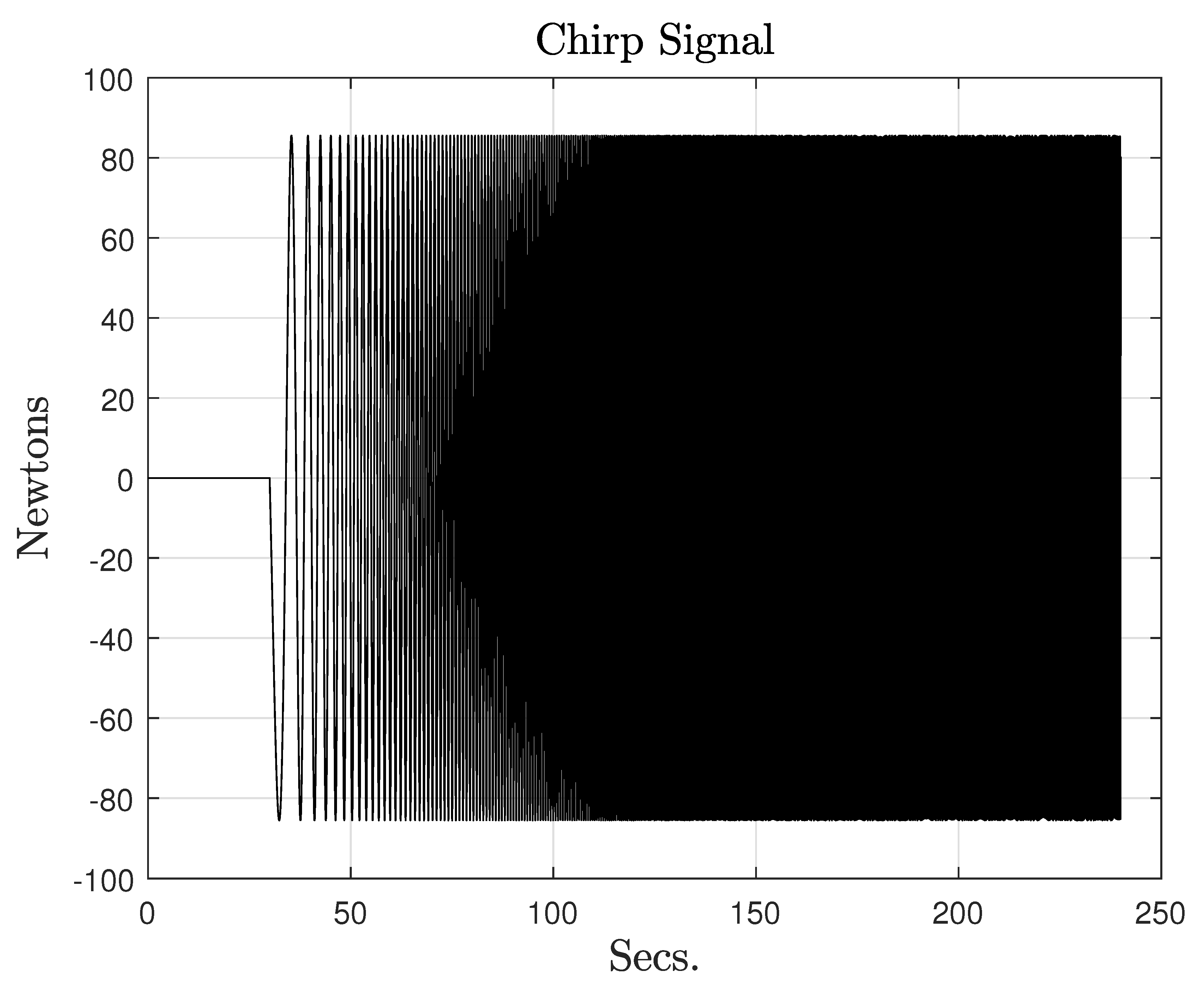
  • “a suitable input signal, u ( t ) is synthesized and input to the experimental system,”
  • “the input signal, u ( t ) and resulting output signal, y ( t ) are recorded,”
  • “an identification algorithm is used to determine the optimal parameter vector, which minimizes some error metric between the actual measured output y ( t ) and that produced by the identified parametric model y ^ ( t | θ ) .”

2.1. Time-Domain Data

The most usual way to identify models is by using input and output time-domain signals: Z N = { u ( 1 ) , y ( 1 ) , , u ( N ) , y ( N ) } . A continuous-time linear time-invariant model can be written as
G ( s , θ ) = b 0 s m + b 1 s m 1 + + b m s n + a 1 s n 1 + + a n
where s is the Laplace variable, and θ comprises the model parameters, i.e., θ = [ b 0 b m , a 1 a n ] . The simulated output, for a particular set of parameters, can be defined as follows:
y ^ ( t | θ ) = G ( p , θ ) u ( t )
where p denotes the differentiation operator. The parameters are then estimated by minimizing a loss function J ( θ ) (also denoted as the error metric) [8,14,15,16,17]:
θ ^ N = arg min θ J ( θ ) ,
where the error metric used in this work is the Normalized Root Mean Squared Error (NRMSE) [17]:
J ( θ ) = N R M S E = t = 1 N y ( t k ) y ^ ( t k | θ ) t = 1 N y ( t k ) y ¯ ( t k )
with y ( t k ) the discrete time measured output data, y ¯ ( t k ) is its mean, and y ^ ( t k | θ ) is the discrete time predicted response of the model. Other error metrics are the mean squared error (MSE), and the mean absolute percentage error (MAPE) [16].

2.2. Frequency-Domain Data

It is also possible to identify continuous-time (or discrete-time) transfer function models from frequency domain data when the data are given in the frequency domain as Fourier transforms of their time-domain counterparts (see [16] Section 7.7 and [14,18]). One approach to estimate continuous-time transfer functions with frequency response measurements uses Sanathanan and Koerner (SK) and instrumental variable (IV) iterations with orthonormal rational basis functions (OVFs). This technique uses frequency response measurements of a MIMO system H ( j ω i ) C p × m for i = i , , l . The goal is to estimate an MIMO system G ^ o ( s ) by minimizing the cost function:
J = i = 1 l W ( j ω i ) ( G ^ o ( j ω i ) H ( j ω i ) ) 2
where W ( j ω i ) is an optional weighting function. G ^ o ( s ) = N ( s ) / d ( s ) is a rational function with d ( s ) : C 1 C 1 and N ( s ) : C 1 C p × m . This algorithm is fully described in [18]. It can also handle grey-box models, i.e., transfer functions with parameter constraints; these constraints can be fixed or bounded numerator or denominator coefficients, where the values of these coefficients can origin from physical considerations. In that work, we can note that the identification procedure contrasts sharply with the time-domain case, and additional issues may present in this methodology, such as numerical issues, or lack of convergence to a local minimum. The work proposed in [18] aims to solve some of these numerical issues.
Some studies propose the use of a frequency domain estimation methodology to identify discrete-time transfer function models, for example in [19]. In that work, the authors estimate the transfer function for a single-body WaveStar wave energy converter with a single rotational degree of freedom. Then, using the identified model, an LTI energy maximizing controller is developed. In order to do the system identification they used observed data taken from a numerical WEC-Sim model. This observed data consists of five experiments, i.e., W n = { D ( 1 ) , , D ( n ) } , with n = 5 , where each element corresponds to an experiment with an input signal with same shape (chirp signal) but different amplitude, and its corresponding output signal. The Fourier transforms of each dataset (experiment) input and output signals are computed ( U n , Y n , respectively), and then the empirical transfer functions are estimated for each experiment:
H ^ n ( j ω ) = Y n ( j ω ) U n ( j ω )
where H ^ n is the n th empirical transfer function estimate (ETFE), Y n and U n are the frequency responses of the n th dataset D ( n ) output and input signals, respectively. Then, the averaged frequency response (AFR) H ¯ ( j ω ) is calculated by averaging the frequency response of all of the ETFEs:
H ¯ ( j ω ) = Re 1 n Re { H ^ n ( j ω ) } n + j Im 1 n Im { H ^ n ( j ω ) } n
After that, the methodology described in [16] Section 7.7 and [18] is used to obtain the discrete-time transfer function estimate G ^ o ( j ω ) , using the AFR H ¯ ( j ω ) as primary data.

2.3. Wave Energy Data Sources

In the context of wave energy, the recorded data for system identification can be originated from two sources: real wave tank tests and numerical wave tank simulations.
Some wave tank facilities consists of wave makers at one end of the wave tank, an absorbing beach, placed at the other end of the wave tank, an adjustable depth floor, which can be set with different depths, and a data logging setup to record the generated data. Figure 1 shows one of the two ocean basins in the LiR National Ocean Test Facility in Cork, Ireland [20].
There are several techniques to implement NWT:
  • Linear potential theory,
  • nonlinear boundary-element methods (BEMs),
  • smooth particle hydrodynamics (SPH), and
  • computational fluid dynamics (CFD).
LPTs are the most low-fidelity/high-speed methods, and this include frequency-domain, Cummins equation time-domain and its extensions, such as the Nonlinear Forude–Krylov (NLFK) approach. On the other hand, CFD are the most high-fidelity/low-speed methods [21], they offer fully nonlinear hydrodynamic calculations by solving numerically the Navier–Stokes equations.
None of both RWT and NWT setups are perfect, they have advantages and disadvantages inherent to their compositions. The disadvantages of both setups are explained below. Note that the disadvantage of one setup is the advantage of the other setup.
RWT disadvantages:
  • “Significant cost and the need for a physical prototype” [13].
  • Generally, prototypes are not full scale, which introduces scaling effects in the experiments [13].
  • “Measurement errors are present” [8].
  • For free surface elevation to body motion models, there may be limitations on the range of excitation signals available [13].
  • “Tank wall reflections may further limit the range and duration of viable tests” [13].
  • The only way to constraint different modes of motion is with mechanical restraints, which can add friction and alter the device dynamics [13].
NWT disadvantages:
  • “All NWTs are implemented by utilizing mathematical models, which necessarily are an approximation of the real system under study” [8].
  • “Furthermore, the approximated equations utilized are resolved with numerical techniques, which introduce additional numerical errors. As a result, a NWT simulation does not completely correspond to the time-evolution of the real system” [8].
  • “LPT-based NWTs assume small amplitude oscillations. This is a major limitation of this modelling approach, since WECS are designed to operate over a wide range of sea conditions where large amplitude motions will result from energetic waves or sustained wave/WEC resonance. At this expanded amplitude range, the linearising assumptions are invalid, as nonlinear effects become relevant” [13].
  • “CFD-based simulations take excessively long time to perform the numerical computation of the response. Typical computation times can be up to 1000 times the simulation time” [13].
In this work, we use RWT tests to gather the data for the identification process. In Section 3, a detailed description of the data logging setup is given.

2.4. WEC Models

Figure 2 shows the forces applied to wave energy converters, it only takes into account excitation and input forces. η is the free surface elevation, and h e x ( t ) is the excitation force kernel, the rest of signals are defined in Section 1. Depending on the forces applied to excite the system, it is possible to obtain two different WEC models: free surface elevation (FSE) to body motion, and input force to body motion.
In the FSE to body motion case, wave excitation experiments—which produce the fluid excitation forces f e —are used to provide two time series vectors, one containing the FSE (the input) and the other the body displacement (the output). In this identified model, the FSE at the body’s centre of mass is considered as input. In this modeling methodology, the input signal is constrained by the laws of fluid dynamics, i.e., an upper bound on the wave frequency content, for example.
In the input force to body motion case, PTO/control force experiments ( f u ) are used to identify the model. The two time series vectors produced by these experiments contain the input force (the input) and the other the body displacement (the output). An almost total freedom over the choice of input signal can be obtained with the input force experiments, the only limitation being the nature of the force realisable by the PTO system [13].
In the present work, we use the input force to body motion approach, where the input force is given by the PTO system f u , while the excitation and the mooring forces are zero, i.e., f e = 0 and f m = 0 , respectively. The main advantage of using this forced (PTO) response approach is that it allows considerably more freedom in the choice of input signal to be applied to the system and can elicit responses and fluid structure interactions beyond those achievable with wave excitation alone. In this regard, “it is important to ensure that the input signal covers the frequency range of interest and that input power is applied to the parts of the spectrum where the identified model is required to perform well” [13]. In addition, the input signal should cover the representative amplitude range of normal operation, so that a representative linear model [22] is achieved, rather than one which is based only on small-signal analysis.

3. Case Study

The system under study was a three-body hinge-barge wave energy converter. Figure 3 shows the hinge-barge (HB) device which consists of the fore, central and aft bodies, two linear motors with 255 N max. force manufactured by LinMot, two load cells connected to the motors to measure the applied forces, and two rotary encoder sensors to measure the relative angles between the fore and central, and aft and central, bodies. The experiments were conducted by applying a set of excitation signals to each motor, separately, and recording the angles of both encoders. The experimental tests were carried out in one of the two ocean basins in the LIR National Ocean Test Facility in Cork, Ireland. The data logging setup is shown in Figure 4. It consist of rotary encoder and load cell sensors, a data acquisition system (DAS), a main computer to control the DAS, and another computer to control the originated waves. The dimensions of the wave tank were 25 m × 15 m × 1 to 2.5 m deep. The wave tank was equipped “with 80 hinged force feedback paddles capable of a peak wave generation condition of Hs = 0.16 m, Tp = 1.4 s and Hmax = 0.32 m, making it suitable for circa. 1/50 scale operational conditions. The paddles are placed on two sides of the basin with making wave direction adjustable by more than 100 degrees. It had a general depth of 1 m with a 11.2 m × 10 m deep section equipped with a movable floor plate to allow the water depth to be adjusted between 1 and 2.5 m depth. Active or passive wave absorption was present allowing improved wave condition and shorter settling time” [20].
The main computer uses dSPACE to compile the models and to control the DAS.
The HB device belongs to the attenuator class of devices. Other hinge barge devices include the M-Ocean [23], M4 device [24] as well as other devices which achieved some degree of deployment such as Seapower [25] deployed in Galway bay 2016, the McCabe Wave Pump (deployed in the Shannon estuary in 1996) and perhaps, most famously, the Pelamis device [26].
Indeed, the three-bodied device in this study is the direct descendant of the original McCabe Wave Pump. The original McCabe wave pump consisted of three rectangular steel pontoons hinged together across their beam. “The pontoons move relative to each other with the waves. A damper plate is attached to the central pontoon, which ensures that it stays still as the fore and aft pontoons move relative to the central pontoon by pitching about the hinges. Energy is extracted from the rotation about the hinge points by linear hydraulic pumps mounted between the central and two outer pontoons near the hinges” [27].
Hinge-barge WECs, being attenuators, are particularly suited to areas where waves are relatively unidirectional, such as estuaries, etc. The work reported in the paper is based on the continuation of a project in conjunction with the Wave Energy Corporation of America, who are developing a hinge-barge device. Therefore, the available prototype device was specifically a hinge-barge form.
The relevance of this type of WECs is important since “they have been proved to have the highest wave energy conversion efficiency and good survivability for a given volume of machine without having to rely on fixed frames of reference” [28].
The current 1:20 scale device was built by the Wave Energy Conversion Corporation of America (WECCA) (who also submitted a 1:50 scale model for the wave energy prize [29]. The device was significantly modified as part of the current BenchWEC project with the addition of two PS01-37x120F-HP-C LinMot motors so that advanced modelling and control techniques could be investigated.

4. Results

The model structure chosen for the identification process is a continuous-time linear time invariant structure. This is the simplest model structure; nevertheless, it has significant precedent due to the number of linear controllers for WECs available in the literature. As stated in Section 2, the input excitation signal should cover the complete range of frequencies and amplitudes of normal system operation in order to get a model with an ability to generalise well. In [13], the authors discuss the specification of the system input signal. They propose three different signals which can be used for specific purposes, i.e., chirp, random amplitude random period (RARP) and multisine signals, and give the desired properties of the input signal in each case:
  • “Good coverage of the frequencies where the system has a significant non-zero frequency response,”
  • “good coverage of the full input and output signal ranges (if the system is nonlinear),” and
  • “economic use of the test time.”
In this work, wave excitation tests were conducted to get the natural resonance frequency of the HB device, and this information was used to establish the operational range of frequencies of the device. A set of chirp signals was used for input excitation, with a linear frequency sweep from 0.5 to 8 rad/s, and five different amplitudes:
I E S = { 37 , 53 , 85 , 102 , 134 } N .
The chirp signals used as inputs in the system identification process are the signals measured by the load cells in the hinge-barge device as described in Section 3.
Five different datasets were recorded using each (measured) input signal in the I E S set:
W n = { D ( 1 ) , , D ( n ) } ,
with n = 5 , where each element D ( · ) corresponds to an experiment with an input signal defined by I E S , and its corresponding output signal. The Fourier transforms of the input and output signals in each dataset are computed ( U n , Y n , respectively), in order to estimate the empirical transfer functions of each experiment (see Equation (7)).
Figure 5 shows a chirp signal with an 85 N amplitude.

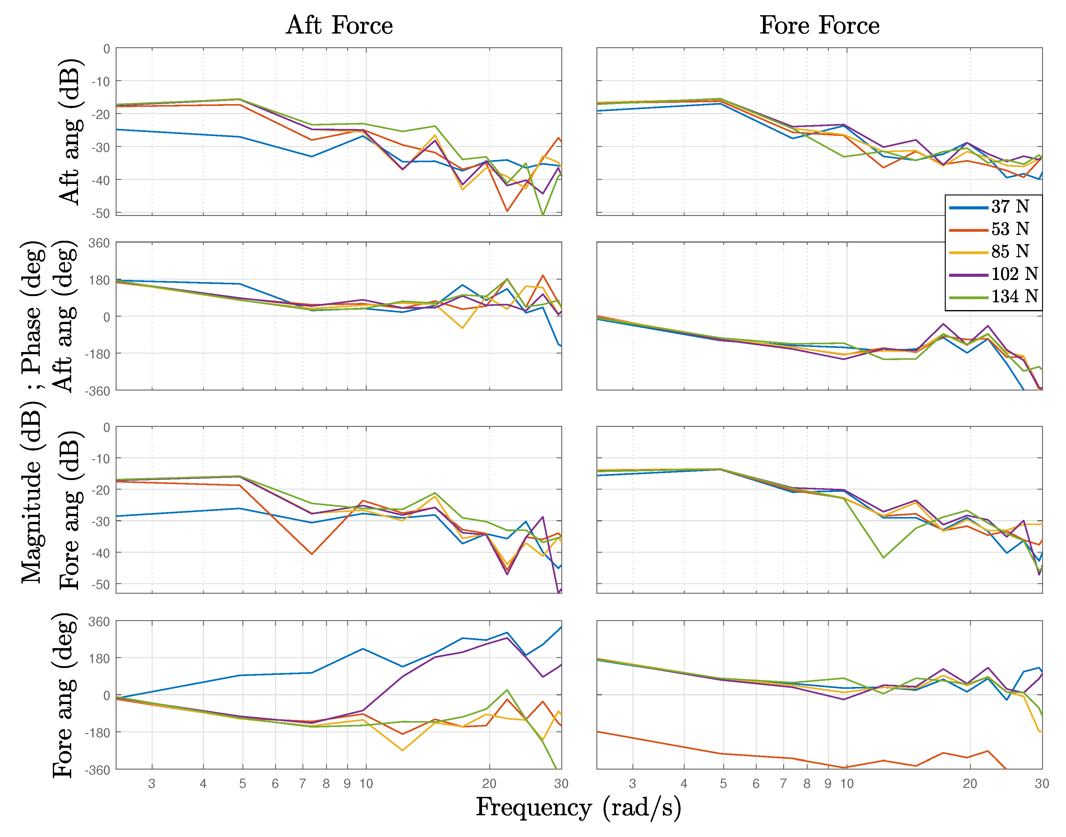
4.1. Data Preprocessing

Experimental data may have flaws of several types, such as uncalibrated sensors (offsets), leading and/or trailing null information (for synchronization purposes), different sample periods between inputs and outputs, non-constant sample period in the same input and/or output set, and missing information (due to other demanding tasks in the operating system); thus, it is necessary to do some data preprocessing to alleviate these problems to the greatest extent possible. Figure 6 shows some of the problems found in the recorded data for the HB WEC.
Graph (a) in Figure 6 shows the angle measurements in the aft barge sensor with a chirp input signal of 85 N amplitude applied to the aft linear motor. In graph (b) of the same figure, there are two segments of missing information in the force measurements of the fore body. The input excitation is a chirp signal with an amplitude of 53 N applied to the fore linear motor. Each segment has missing information of around one second duration.

4.2. Linear Model Estimation

The first step in the model identification process was to establish if the system can be approximated with a linear model as opposite to a nonlinear model. In this respect, the ETFE of each experiment dataset was calculated as shown in Equation (7). Figure 7 shows the Bode plots of the frequency response for each ETFE. Since each ETFE is an MIMO model, this figure shows an array of plots where each plot shows the frequency response (amplitude and phase) of one I/O pair. The input signals are the aft and fore force signals, and the output signals are the aft and fore angle signals. The units of the amplitudes are in decibels (dB), and the units of the phases are in degrees (deg). It can be noticed that the models have a similar frequency response, except for some of the smaller input signal amplitudes, i.e., 37 and 53 N. This is due to the lower signal-to-noise ratios for these signals.
In order to get an accurate linear model, several identification strategies were used. They are described as follows.
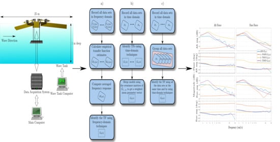
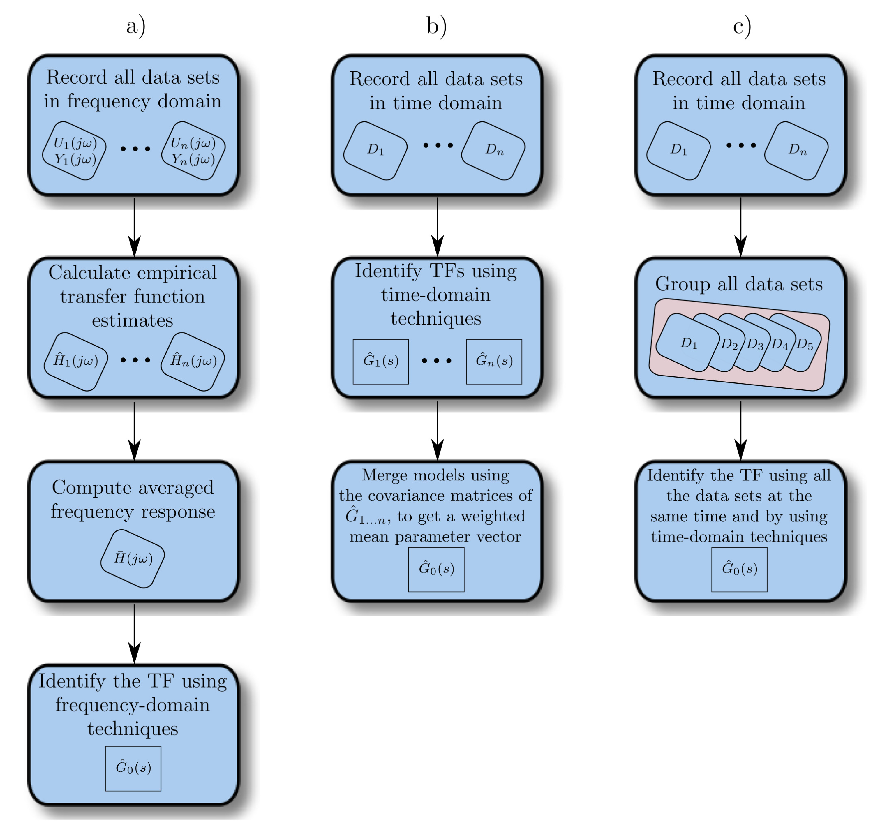
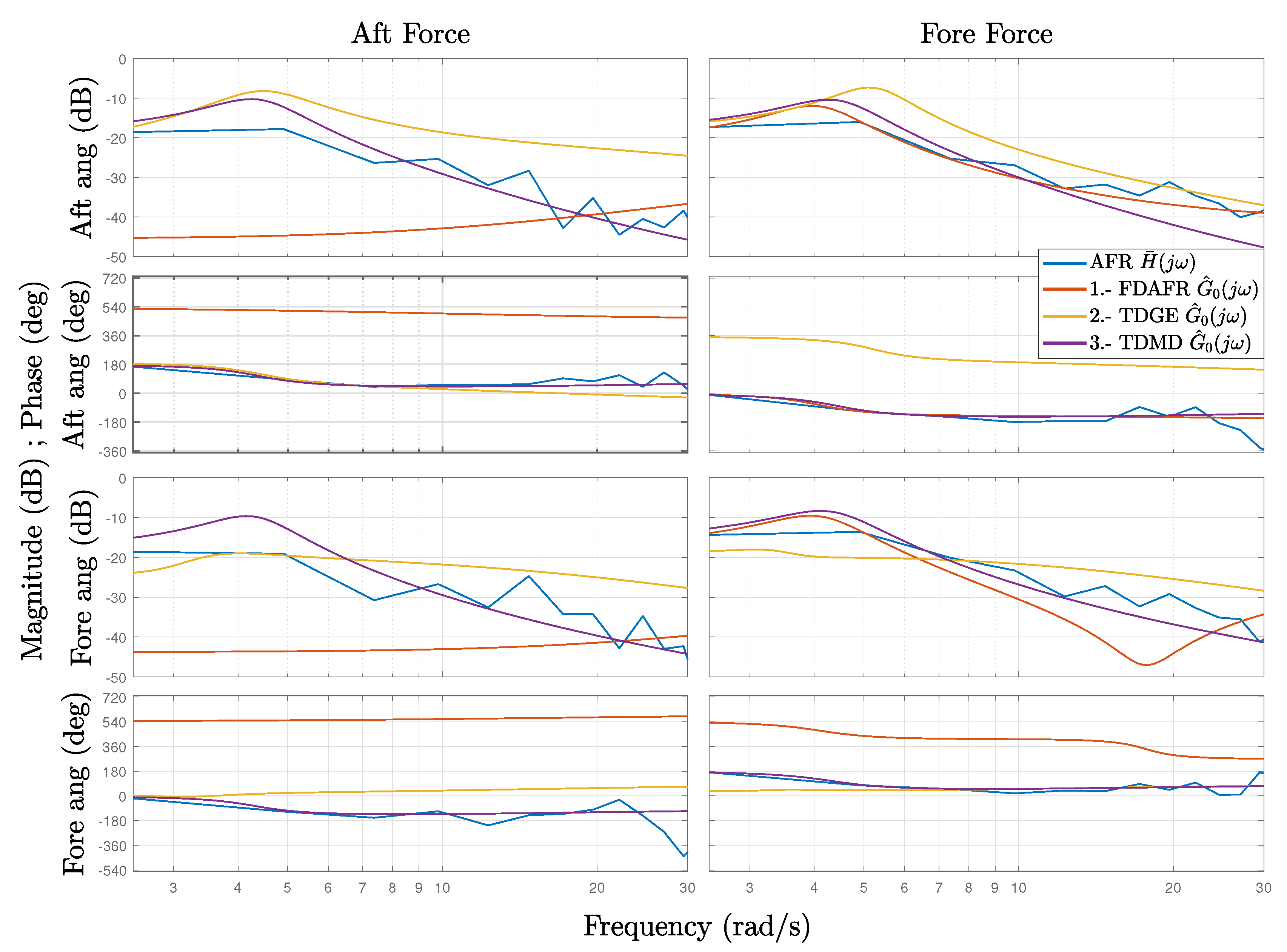
  • Model identified using frequency-domain SIT and averaged frequency response (FDAFR). See Figure 8a.
    • Calculate the ETFE as shown in (7) for each dataset in W n (see Equation (10)).
    • Compute the averaged frequency response of all of the ETFEs.
    • The model is identified by using frequency domain SIT that employs the averaged frequency response as the primary data input (see [16] Section 7.7 and [14,18]).
    Note that this is the same methodology as employed in [19].
  • Model identified using time-domain SIT and a global estimate (TDGE). See Figure 8b.
    • Estimate (identify) the continuous transfer function for each dataset in W n using time-domain SIT.
    • Compute a global estimate using the covariance matrices of each estimated transfer function to get a weighted mean parameter vector.
  • Model identified using time-domain SIT and merged data (TDMD). See Figure 8c.
    • Merge the data for all the recorded input and output signals.
    • Estimate the continuous transfer function with these merged data, using the time-domain SIT described in Section 2.1. When estimating the transfer function in this way, the prediction error vector is formed over the entire collection of experiments, assigning equal weight to observations in each experiment, i.e., the identification is done using all the input and output signals of the five experiments ( D 1 , , D 5 ) at the same time.
Each identification strategy produces a transfer function matrix (TFM) H ^ i ( s ) R p x q ( s ) , with i = 1 , 2 , 3 , and p = q = 2 , where each element in the matrix corresponds to a transfer function between each input signal (aft and fore forces) and each output signal (aft and fore angles):
H ^ i ( s ) = Y ^ A ( s ) U ^ A ( s ) Y ^ A ( s ) U ^ F ( s ) Y ^ F ( s ) U ^ A ( s ) Y ^ F ( s ) U ^ F ( s )
where ^ denotes an estimate, Y x and U x are the Laplace transforms of the output and input signals, respectively. Subscripts A and F stand for aft and fore bodies, respectively.
The optimal transfer function order was achieved by using the parsimony principle, which states that “the model should contain the smallest number of free parameters required to represent the true system adequately” [30]. The best results were obtained using four poles and three zeros for each transfer function in (11), i.e.,
G ^ x ( s ) = b 0 s 3 + b 1 s 2 + b 2 s + b 3 s 4 + a 1 s 3 + a 2 s 2 + a 3 s + a 4 .
The fit criterion is calculated using the NRMSE metric:
F i t = 100 ( 1 N R M S E )
F i t is a percent value and varies between (poor fit) to 100 (perfect fit) [17].
The fit criterion (12) is used to compare the accuracy of each identification strategy. It is given as a 2 × 2 matrix where each percent value corresponds to the fit metric for each transfer function element in (11).
Table 1 shows the fitting percent for each strategy. In the first strategy case, the identification was made with the AFR H ¯ ( j ω ) data as it is shown in Figure 8a; thus, the Fit values consist of a single matrix R 2 × 2 . In the second case, the identification was made with each dataset in W n (see Equation (10)); thus, the Fit values consist of five matrices R 2 × 2 . As it is shown in Figure 8c, the identification took into account each dataset in W n at the same time; therefore, the Fit values consist of five matrices R 2 × 2 . We can note that the FDAFR strategy delivers the poorest results. Therefore, it can be inferred that the FDAFR strategy is not well suited for WEC MIMO linear models. TDGE strategy delivers good individual results as can be seen in Table 1. However, when merging the models, the global estimate is not so good because the TDGE strategy is very sensitive to significant differences in the covariance matrices of each individual model. This is the case for this particular WEC; thus, the global estimate is ill-conditioned. The Fit values shown for the TDMD strategy are the error metrics using each input signal in the set IES, and its corresponding output signal given by the identified model against the real output signals given by the recorded datasets D 1 , , D 5 . As can be noted, the TDMD strategy gives accurate results for almost all the input-output data.
Figure 9 shows the AFR H ¯ ( j ω ) signal and the Bode plots for each identification strategy. It is clear that only the TDMD strategy is able to accurately approximate the AFR signal.
Table 2 shows the average of the five (see Equations (9) and (10) F i t matrices for the TDMD strategy. The lower bound is above 74% and the best value is above 80%.
The identified transfer function matrix given by the TDMD strategy is shown as follows.
H ^ 3 ( s ) = Aft   force Fore   force Aft   angle 0.1201 s 3 3.5174 s 2 15.0458 s 0.809 s 4 + 8.7875 s 3 + 31.992 s 2 + 135.124 s + 0.2377 0.09032 s 3 + 2.5934 s 2 + 3.9625 s + 0.2261 s 4 + 3.609 s 3 + 23.18 s 2 + 34.751 s + 3.148 Fore   angle 0.1637 s 3 + 2.273 s 2 + 0.2364 s 0.003216 s 4 + 1.735 s 3 + 18.66 s 2 + 0.7318 s + 0.01862 0.2311 s 3 3.0973 s 2 1.065 s + 0.02726 s 4 + 2.3392 s 3 + 19.379 s 2 + 6.9114 s + 0.01596

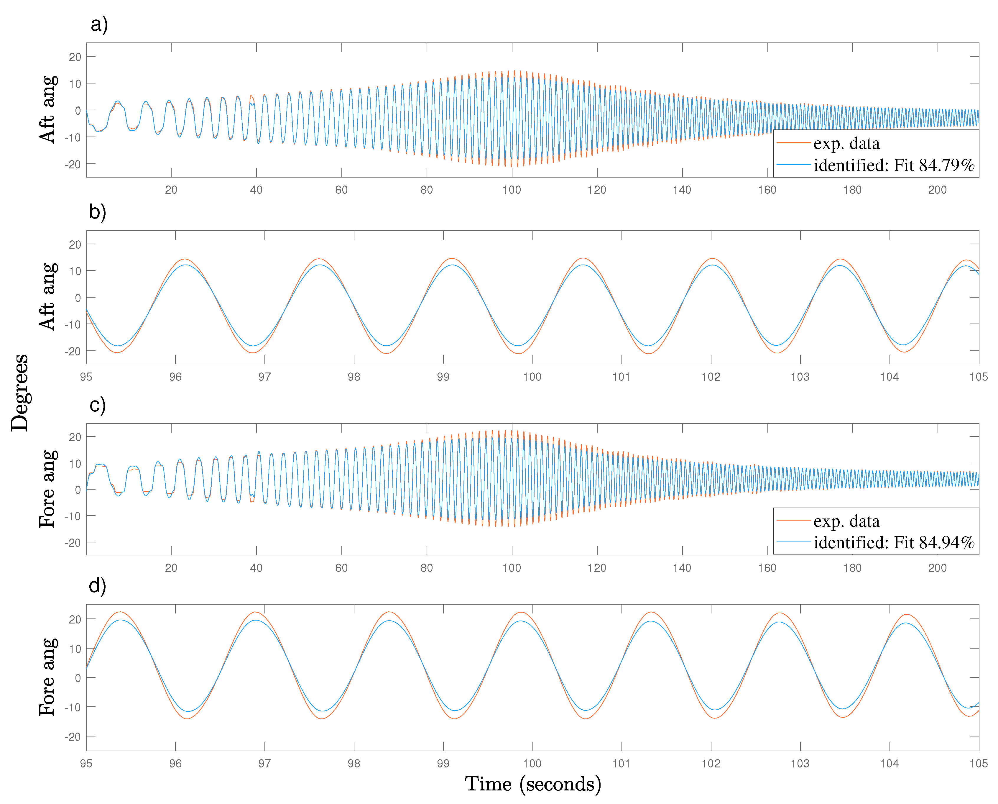
4.3. Model Validation

Since the models obtained with the first and the second strategies are ill-conditioned, only the model obtained with the third strategy was validated against a chirp signal with the same frequency sweep but with 69 N amplitude. Figure 10 shows the comparison between the experimental data output and the identified model output. It can be seen that the F i t value is above 84%. Table 1 shows the Fit values of the simulated responses for each input excitation signal in the set IES. It can be noticed that the simulated response for the 37 N input signal is not precise, due to small signal-to-noise ratio.

5. Conclusions and Future Research Directions

A linear model was obtained using system identification techniques based on experimental data. In order to do the identification, it was necessary to preprocess the data first. Several strategies were developed to get an accurate linear model. Merging the models obtained with each input-output test data into a global estimate did not give good results because the single models have significant differences in their covariance matrices. It was found that merging the data of all the recorded input and output signals, and then estimating the transfer function with these data, gives the best results.
The identified model was validated against a chirp signal with a different amplitude. The simulated response of the estimated linear model has a fidelity of 84% with this new signal.
Future research directions include the development and experimental tests of linear controllers using the linear model developed in this work.

Author Contributions

Investigation, F.J.-L. and B.F.; Writing—original draft, F.J.-L.; Writing - review & editing, B.F., J.M. and J.V.R.; Funding acquisition, J.V.R.; Project administration, J.M. and J.V.R.; Resources, J.M. and J.V.R.; Software, F.J.-L.; Supervision, J.M. and J.V.R.; Validation, B.F. All authors have read and agreed to the published version of the manuscript.

Funding

This paper is based upon work supported by Science Foundation Ireland under Grant no. 13/IA/1886.

Conflicts of Interest

The authors declare no conflict of interest.

References

  1. Ringwood, J.; Bacelli, G.; Fusco, F. Energy-Maximizing Control of Wave-Energy Converters: The Development of Control System Technology to Optimize Their Operation. IEEE Control Syst. Mag. 2014, 34, 30–55. [Google Scholar]
  2. Ringwood, J. Wave energy control: Status and perspectives 2020. In Proceedings of the IFAC World Congress 2020, Berlin, Germany, 11–17 July 2020. [Google Scholar]
  3. Ljung, L. Perspectives on system identification. Annu. Rev. Control 2010, 34, 1–12. [Google Scholar] [CrossRef] [Green Version]
  4. Cummins, W. The impulse response function and ship motions. Schiffstechnik 1962, 47, 101–109. [Google Scholar]
  5. O’Cathain, M.; Leira, B.J.; Ringwood, J. Modelling of Multibody Marine Systems with Application to Wave-Energy Devices. In Proceedings of the 7th European Wave and Tidal Energy Conference, Porto, Portugal, 11–13 September 2007. [Google Scholar]
  6. Paparella, F.; Bacelli, G.; Paulmeno, A.; Mouring, S.E.; Ringwood, J.V. Multibody Modelling of Wave Energy Converters Using Pseudo-Spectral Methods With Application to a Three-Body Hinge-Barge Device. IEEE Trans. Sustain. Energy 2016, 7, 966–974. [Google Scholar] [CrossRef] [Green Version]
  7. Paparella, F.; Ringwood, J.V. Optimal Control of a Three-Body Hinge-Barge Wave Energy Device Using Pseudospectral Methods. IEEE Trans. Sustain. Energy 2017, 8, 200–207. [Google Scholar] [CrossRef]
  8. Giorgi, S.; Davidson, J.; Jakobsen, M.; Kramer, M.; Ringwood, J.V. Identification of dynamic models for a wave energy converter from experimental data. Ocean Eng. 2019, 183, 426–436. [Google Scholar] [CrossRef]
  9. Bacelli, G.; Coe, R.; Patterson, D.; Wilson, D. System Identification of a Heaving Point Absorber: Design of Experiment and Device Modeling. Energies 2017, 10, 472. [Google Scholar] [CrossRef]
  10. Cho, H.; Bacelli, G.; Coe, R. Linear and Nonlinear System Identification of a Wave Energy Converter. In Proceedings of the 6th Marine Energy Technology Symposium, Washington, DC, USA, 30 April–2 May 2018. [Google Scholar]
  11. Sun, L.; Zang, J.; Stansby, P.; Carpintero Moreno, E.; Taylor, P.H.; Eatock Taylor, R. Linear diffraction analysis of the three-float multi-mode wave energy converter M4 for power capture and structural analysis in irregular waves with experimental validation. J. Ocean Eng. Mar. Energy 2017, 3, 51–68. [Google Scholar] [CrossRef] [Green Version]
  12. Jaramillo-Lopez, F.; Flannery, B.; Murphy, J.; Ringwood, J.V. Black-box Modelling of a Three-Body Hinge-Barge Wave Energy Device via Forces Responses. In Proceedings of the 4th International Conference on Renewable Energies Offshore, Lisbon, Portugal, 12–15 October 2020. [Google Scholar]
  13. Davidson, J.; Giorgi, S.; Ringwood, J.V. Identification of Wave Energy Device Models From Numerical Wave Tank Data—Part 1: Numerical Wave Tank Identification Tests. IEEE Trans. Sustain. Energy 2016, 7, 1012–1019. [Google Scholar] [CrossRef] [Green Version]
  14. Ljung, L. Identification for control: Simple process models. In Proceedings of the 41st IEEE Conference on Decision and Control, Las Vegas, NV, USA, 10–13 December 2002; pp. 4652–4657. [Google Scholar]
  15. Ljung, L. Experiments with Identification of Continuous Time Models. In Proceedings of the 15th IFAC Symposium on System Identification, Saint-Malo, France, 6–8 July 2009; pp. 1175–1180. [Google Scholar]
  16. Ljung, L. System Identification: Theory for the User, 2nd ed.; Prentice-Hall: Upper Saddle River, NJ, USA, 1999. [Google Scholar]
  17. Ljung, L. System Identification Toolbox for Use with MATLAB: Reference (R2019b); The MathWorks, Inc.: Natick, MA, USA, 2019. [Google Scholar]
  18. Ozdemir, A.A.; Gumussoy, S. Transfer Function Estimation in System Identification Toolbox via Vector Fitting. IFAC-PapersOnLine 2017, 50, 6232–6237. [Google Scholar] [CrossRef]
  19. Garcia-Violini, D.; Pena-Sanchez, Y.; Faedo, N.; Windt, C.; Ringwood, J. LTI energy-maximising control for the Wave Star wave energy converter: Identification, design, and implementation. In Proceedings of the IFAC World Congress 2020, Berlin, Germany, 11–17 July 2020. [Google Scholar]
  20. LIR-NOTF. LIR National Ocean Test Facility, Cork, Ireland. 2020. Available online: http://www.lir-notf.com/wavebasins/ (accessed on 23 June 2020).
  21. Davidson, J.; Costello, R. Efficient Nonlinear Hydrodynamic Models for Wave Energy Converter Design— A Scoping Study. J. Mar. Sci. Eng. 2020, 8, 35. [Google Scholar] [CrossRef] [Green Version]
  22. Davidson, J.; Giorgi, S.; Ringwood, J.V. Linear parametric hydrodynamic models for ocean wave energy converters identified from numerical wave tank experiments. Ocean Eng. 2015, 103, 31–39. [Google Scholar] [CrossRef] [Green Version]
  23. Mocean Energy. Mocean Energy News. 2020. Available online: https://www.mocean.energy/wave-energy-news/ (accessed on 10 April 2020).
  24. Stansby, P.; Carpintero Moreno, E.; Stallard, T.; Maggi, A. Three-float broad-band resonant line absorber with surge for wave energy conversion. Renew. Energy 2015, 78, 132–140. [Google Scholar] [CrossRef]
  25. Seapower. Seapower. 2020. Available online: http://www.seapower.ie/ (accessed on 10 April 2020).
  26. Yemm, R.; Pizer, D.; Retzler, C.; Henderson, R. Pelamis: Experience from concept to connection. Philos. Trans. R. Soc. A 2012, 370, 365–380. [Google Scholar] [CrossRef] [PubMed] [Green Version]
  27. de Almeida, A.; Moura, P. Desalination with wind and wave power. In Solar Desalination for the 21st Century; NATO Security through Science Series; Springer: Dordrecht, The Nertherlands, 2007; pp. 305–325. [Google Scholar] [CrossRef]
  28. Yu, H.; Zhang, Y.; Zheng, S. Numerical study on the performance of a wave energy converter with three hinged bodies. Renew. Energy 2016, 99, 1276–1286. [Google Scholar] [CrossRef]
  29. Offshore Energy. WECCA Completes Scaled Wave Energy Device. 2016. Available online: https://www.offshore-energy.biz/wecca-completes-scaled-wave-energy-device-prize/ (accessed on 10 April 2020).
  30. Soderstrom, T.; Stoica, P. System Identification; Prentice-Hall: Upper Saddle River, NJ, USA, 1989. [Google Scholar]
Figure 1. Ocean basin in LIR National Ocean Test Facility in Cork, Ireland [20].
Energies 13 05129 g001
Figure 2. Forces applied to wave energy converters.
Energies 13 05129 g002
Figure 3. CAD rendering of the three-body hinge-barge wave energy converter.
Energies 13 05129 g003
Figure 4. Wave tank and data logging setup.
Energies 13 05129 g004
Figure 5. Chirp signal with frequency swept from 0.5 to 8 rad/s and 85 N amplitude.
Energies 13 05129 g005
Figure 6. Typical dropouts found in the experimental data. (a) Aft Angle Sensor—85 Newtons; (b) Fore Force Sensor—53 Newtons.
Energies 13 05129 g006
Figure 7. Empirical transfer function estimates.
Energies 13 05129 g007
Figure 8. Strategies for linear identification of a WEC model. (a) Frequency-domain and averaged frequency response—FDAFR. (b) Time-domain and global estimate—TDGE. (c) Time-domain and merged data—TDMD.
Energies 13 05129 g008
Figure 9. Average frequency response (AFR) H ¯ ( j ω ) and identified transfer functions G ^ 0 ( j ω ) for each strategy.
Energies 13 05129 g009
Figure 10. Comparison of modelled and experimental system using a input chirp signal with 69 N amplitude. (a,c) aft and fore angles, respectively. (b,d) zoom to the resonance part for aft and fore angles, respectively.
Energies 13 05129 g010
Table 1. F i t values for each identification strategy.
Input-Output AFR H ¯ ( j ω ) /
Data37 N53 N85 N102 N134 N
FDAFR strategy 4.38 22.04 7.05 26.59
TDGE strategy 28.23 77.67 72.70 73.13 89.74 79.09 87.08 79.33 93.81 88.62 93.78 90.28 93.07 82.49 93.20 82.97 89.19 74.43 80.25 73.35
TDMD strategy 54.10 70.36 25.88 70.79 80.85 73.82 79.83 73.70 89.62 87.19 89.10 86.19 91.78 79.29 90.98 77.85 88.44 78.45 88.67 76.73
Table 2. Average F i t values for the TDMD strategy.
80.96 77.82 74.89 77.05

