Article

Disturbance Observer and L2-Gain-Based State Error Feedback Linearization Control for the Quadruple-Tank Liquid-Level System

School of Automation, Qingdao University, Qingdao 266071, China
*
Author to whom correspondence should be addressed.
Energies 2020, 13(20), 5500; https://doi.org/10.3390/en13205500
Submission received: 29 August 2020 / Revised: 6 October 2020 / Accepted: 10 October 2020 / Published: 20 October 2020

Abstract

:
This paper proposes a fresh state error feedback linearization control method with disturbance observer (DOB) and L 2 gain for a quadruple-tank liquid-level system. Firstly, in terms of the highly nonlinear and strong coupling characteristics of the quadruple-tank system, a state error feedback linearization technique is employed to design the controller to achieve liquid-level position control and tracking control. Secondly, DOB is purposed to estimate uncertain exogenous disturbances and applied to compensation control. Moreover, an L 2 -gain disturbance attenuation technology is designed to resolve one class of disturbance problem by uncertain parameter perturbation existing in the quadruple-tank liquid-level system. Finally, compared with the classical proportion integration differentiation (PID) and sliding mode control (SMC) methods, the extensive experimental results validate that the proposed strategy has good position control, tracking control, and disturbance rejection performances.

1. Introduction

Accurate liquid-level control in an interconnected multitank system is a difficult problem for various industrial process devices. This is an important issue because it is applicable to many industries, such as wastewater treatment plants, chemical plants, biomedical plants, food processing plants, power plants, filtration devices, and other modern process industries [1]. In addition, the liquid-level control is used to test and analyze the benchmark problem of advanced nonlinear observer and controller. From the perspective of liquid-level control, the process is very interesting because it not only involves a lot of multivariable control instances, but also mathematical models—nonlinear and highly coupled. Liquid level of four tanks can be controlled in real-time through a number of sensors installed on the devices. Dynamic properties, which are change of expectation level and dynamic response speed, and some related control performances can be controlled by changing pump flow. In the past decades, many scholars have studied the control problem of this process and conducted experimental tests in a laboratory [2,3,4].
At present, the control strategies of the multitank liquid-level system mainly concentrates on the following aspects, for instance, proportion integration differentiation (PID) control [5,6,7], predictive control [8,9], fuzzy control [10], backstepping control [11,12], and sliding mode control (SMC) [13,14]. In addition to the above, there are some other methods used in the multiple-tank liquid-level system. The paper of [15] proposed a method of energy-shaping for a three-tank liquid-level system. The authors of [16] presented the design and implementation method of a robust decentralized proportion integration controller based on a predefined transfer function model. In recent years, some scholars have proposed the idea of feedback linearization [17] for nonlinear systems with multi-input and multioutput (MIMO). Using the discrete storage function and the secondary supply rate, the nondissipative condition of the quadruple-tank liquid-level system was given. On this basis, the state feedback control law to ensure the nondispersibility of the system was obtained [18]. For every steady state feedback gain [19], a 2-DOF (degrees of freedom) MIMO proportional integral (PI) derivative controller was designed based on noniterative linear matrix inequality. The applicability and accuracy of the proposed decentralized control method for nonlinear systems were verified by simulation. In [20], the robust input–output feedback linearization control technology of induction motor was studied. The results showed that the robustness of the controller to parameter changes was significantly increased. The paper of [21], the state feedback linearization method was used to transform the nonlinear average dynamic of the inductor current in the converter into the linear average dynamic of the inductor current in the virtual grid. The experimental results showed that the system had the characteristics of fast recovery and zero steady-state output voltage error under the large signal interference of input voltage and output power. A current control strategy based on feedback linearization [22] was proposed to reduce the difficulties in controller design for nonlinear systems with a high coupling state. The problem of output feedback sampled data stabilization for a class of large-scale nonlinear switched systems was studied [23]. Since the system output was only available at the moment of sampling data, a state observer was constructed to estimate the unmeasured states. The set operation was simplified to a simple matrix representation of the region topology set, which was used to constrain the state/output estimation provided by the interval observer method [24]. In [25], a method of combining feedback linearization technique with disturbance observer was proposed. The state feedback control law was used to realize the stability of inductance capacitance inductance (LCL) filter under a wide range of resonant frequency variations. The disturbance observer was designed to counteract the effects of model uncertainties and unknown disturbances, and to achieve asymptotic stability under feedback linearization control.
For systems with MIMO, strong nonlinearity, and unknown perturbations, the simple control algorithms are not enough. Moreover, the disturbance has great influence on the system, which not only affects the accurate tracking of the system, but also threatens the stability of the whole system. Therefore, it is imperative to resolve the disturbance problem. The authors of [26] proposed a nonlinear disturbance observer for the disturbance of external systems, and the global exponential stability of the system was established under certain conditions. Furthermore, the semiglobal stability conditions of the composite controller composed of nonlinear controller and nonlinear disturbance observer were established. A finite time disturbance observer was proposed for three-tank liquid-level systems with mismatched uncertainties. The nonlinear uncertainty was compensated by the finite time disturbance observer [27]. In order to realize the controller in a sensorless control framework, an adaptive interconnected high-gain observer [28] was designed to measure the liquid level of the tank at the bottom and estimate the two constant parameters for the tank-liquid-level system. The control calibration was realized by adjusting two scalar design parameters. The review expressed existing interference/uncertainty, and the attenuation technology guidance and summary were systematical and comprehensive—especially the disturbance observer based control, active disturbance rejection controller (ADRC); interference immunity regulating control; and complex antijamming hierarchical control—then discussed and compared the varying compensation technology usage and design of linear/nonlinear controller in advanced and integrated processes [29]. An integrated backstepping control method based on disturbance observer [12] was proposed for two-tank liquid-level system with external disturbance. It was shown that disturbance observer control and its related methods originated from intuitive practices in many different applications and had wide applications in the industrial field, from traditional mechatronic and motion control to biological process systems and aerospace systems. Compared with other advanced control algorithms, it was one of the few commercialized and industrialized control algorithms.
In the process control system, the multitank liquid-level system has interaction and noninteraction circuits with nonlinear, time-varying, steady, stable, and unstable characteristics. Due to the presence of interactions and uncertainties, multivariable processes are difficult to control over the desired reference. In most cases, intricate control systems provide nonlinear behavior with multiple inputs and multiple outputs, and complex interactions with matched and mismatched uncertainties between manipulation and control variables. In [30], the problem of state and parameter estimation of nonlinear systems was studied by using extended Kitanidis Kalman filter. This method can be used for state estimation and parameter estimation. The authors of [31] defined uncertainty as a combination of unknown interference, parameter uncertainty, measurement error, and ignoring dynamics. Modeling and designing gave us a deeper understanding of the dynamic nature of the problem. Two theorems to determine its application range were given. The authors of [32] proposed an optimization algorithm to estimate the optimal value of Laguerre poles from the input/output measurements. The authors of [33] designed the controller under the known and unknown load torque. Aimed at the load torque disturbance, an observer was proposed to estimate the unknown load torque. The paper of [34], an adaptive disturbance attenuation control based on port-controlled Hamiltonian [35] was designed for two-tank liquid-level system with uncertain parameters. In order to reduce the influence of interference and unmeasurable parameters, an adaptive L 2 interference attenuation technology was integrated. Under the effect of leakage delay, the design of L 2 - L state estimation for delayed neural network of quadruple-tank liquid-level system was considered, and a L 2 - L state estimation criterion based on linear matrix inequalities was proposed [36]. In industrial applications, process delay and interference were considered as the only factors that lead to the deterioration of performance of multivariable systems. Quadruple-tank liquid-level system is a multivariable system, so it needs to control at least two variables. An embedded model control [37] was designed. The embedded model includes stochastic perturbation dynamics that can estimate and correct the uncertainty, variability, and state dependence of electromotive force parameters. Taking the quadruple-tank process as an example, this paper proposed a method based on nominal error updating model: by comparing the measured output of the system with the corresponding nominal output [38]. The main advantage of this method was that it avoided common multivariable model identification and used simple SISO structure, thus reducing the workload of model maintenance. Purposed to the stability of physical and chemical nonlinear processes, a nonfeedback passivation stage control method based on tracking error was proposed [39]. In order to achieve the control goal, the system dynamics formula was expressed as a relaxed (pseudo) Hamiltonian with quadratic storage function under appropriate conditions, and the asymptotic and global convergence of the error dynamics were guaranteed by adding corresponding damping injection. The authors of [40] proposed a smooth switching control method for the quadruple-tank liquid-level system, which resolved the problems of serious sliding mode buffeting and slow transient response in the backstepping control. In [41], a method for generating approximate spatial residuals was proposed, which was excited by the method of set membership and approximate decoupling. The influence of uncertainty on matrix calculation was solved by means of set membership degree method and band position representation method. In addition to the above documents, adaptive actor-critic data-driven model-free tracking reinforcement learning control based on virtual reference feedback tuning, a programmable logic controller (PLC)-based fractional water level control method, and a Takagi–Sugeno fuzzy model based on linear matrix inequality fault-tolerant control were also proposed [42,43,44].
The main contributions of this paper are summarized as follows:
Firstly, in terms of the highly nonlinear and strong coupling characteristics of the quadruple-tank liquid-level system, a state error feedback linearization technique is employed to design the controller to achieve liquid-level position control and tracking control.
Secondly, disturbance observer (DOB) is purposed to estimate uncertain exogenous disturbances and applied to compensation control.
Thirdly, a L 2 -gain disturbance attenuation technology is designed to resolve one class of disturbance problem by uncertain parameter perturbation existing in the quadruple-tank liquid-level system.
The remainder of this paper is organized as follows. Section 2 presents the quadruple-tank liquid-level system dynamics model. Controller design and stability analysis are introduced in Section 3. Experimental results are presented in Section 4. This paper is concluded in Section 5.

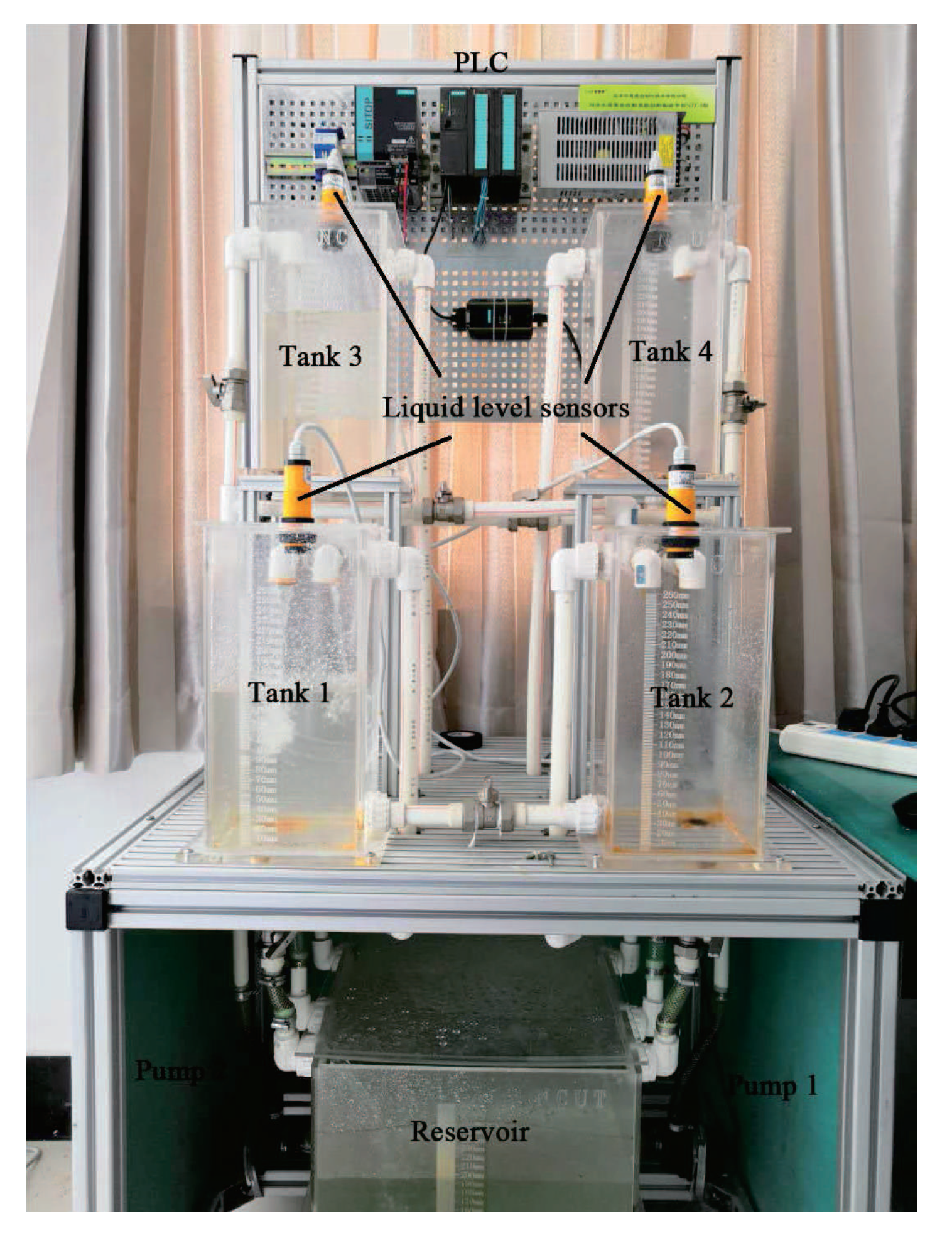
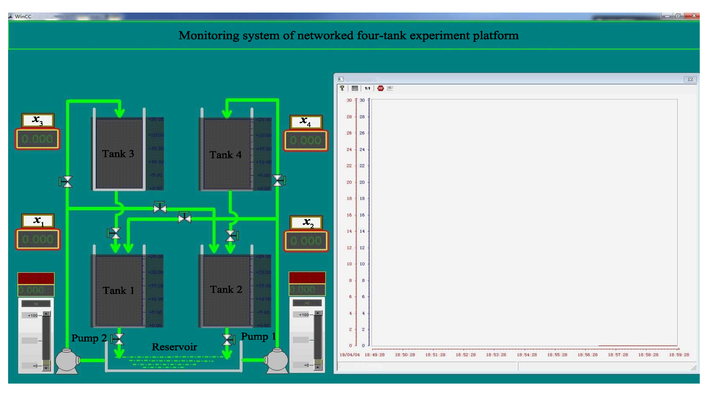
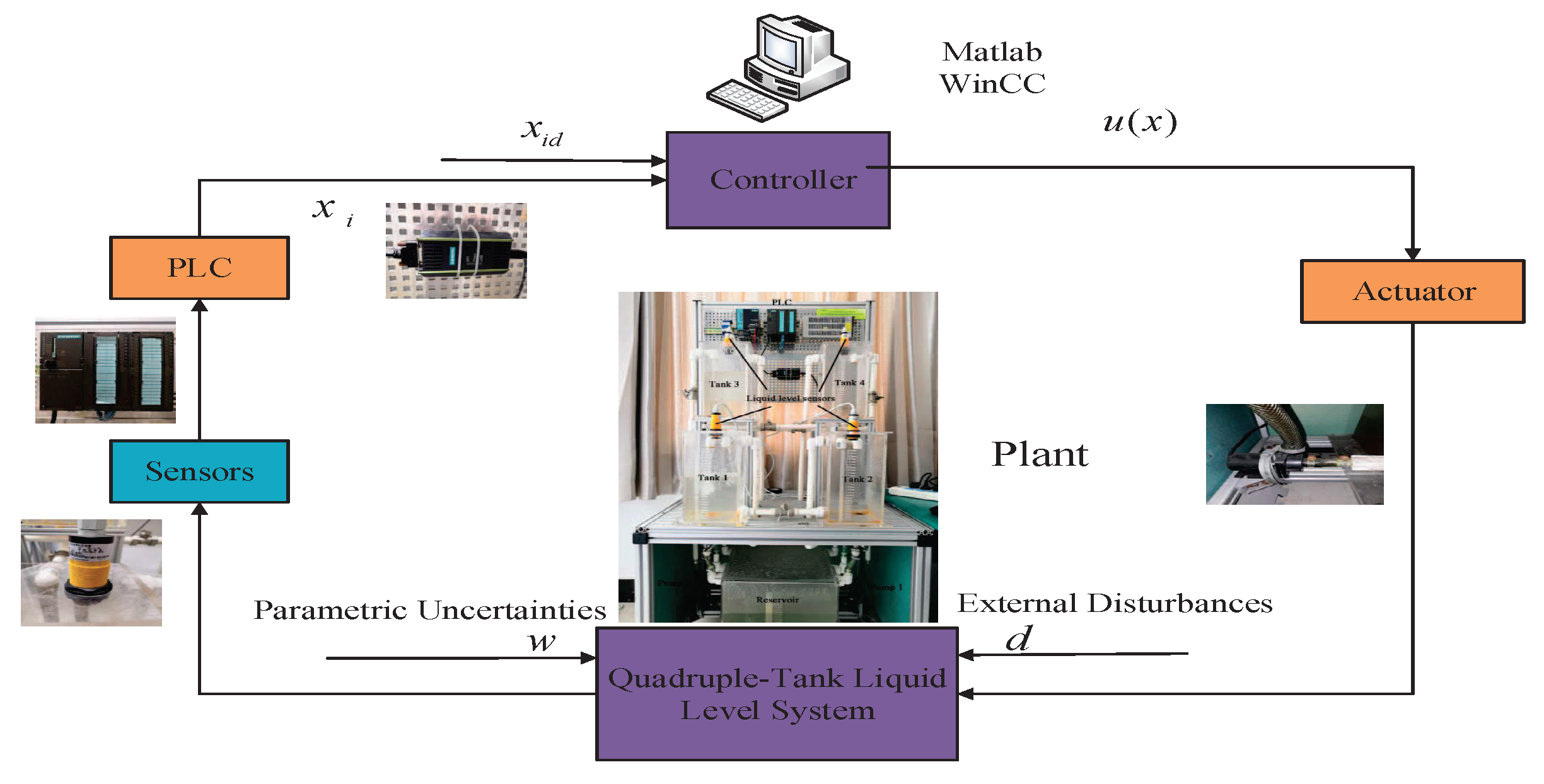
2. Description of Quadruple-Tank System

From Figure 1 and Figure 2 experimental equipment and the schematic diagram are represented for a quadruple-tank liquid-level system. This system consists of four tanks, four level sensors which are located at the top of each tank, two pumps, a reservoir tank, and eight manual valves. In this experimental device, pump 1 feeds Tanks 1,4; and pump 2 feeds Tanks 2,3. The outflow of Tank 3 turns into partial input of Tank 1; the outflow of Tank 4 turns into partial input of Tank 2.
Using Bernoulli’s law, principle of fluid mechanics, and principle of mass conservation, the mathematical model of quadruple-tank liquid-level system [3,8,9,10] can be described by state equations
x ˙ 1 x ˙ 2 x ˙ 3 x ˙ 4 = a 1 A 1 2 g x 1 + a 3 A 1 2 g x 3 a 2 A 2 2 g x 2 + a 4 A 2 2 g x 4 a 3 A 3 2 g x 3 a 4 A 4 2 g x 4 + a 6 a 5 + a 6 · 1 A 1 0 0 a 8 a 7 + a 8 · 1 A 2 0 a 7 a 7 + a 8 · 1 A 3 a 5 a 5 + a 6 · 1 A 4 0 u 1 u 2 ,
where state variable x i is the height of liquid inside the tank i, u j is the control input, A i is the cross section of tank i, and a i is the cross section of the outlet manual valve i, g is the gravitational acceleration. i = 1 , 2 , 3 , 4 . j = 1 , 2 .
In order to express the design steps more concisely and explain the main content of this article, the following constants are defined:
A = a 1 A 1 2 g , B = a 3 A 1 2 g , C = a 6 a 5 + a 6 · 1 A 1 , D = a 2 A 2 2 g , E = a 4 A 2 2 g , F = a 8 a 7 + a 8 · 1 A 2 , G = a 3 A 3 2 g , H = a 7 a 7 + a 8 · 1 A 3 , I = a 4 A 4 2 g , J = a 5 a 5 + a 6 · 1 A 4 .
Based on the situation above, the quadruple-tank liquid-level system (1) can be rewritten as
x ˙ 1 x ˙ 2 x ˙ 3 x ˙ 4 = A x 1 + B x 3 D x 2 + E x 4 G x 3 I x 4 + C 0 0 F 0 H J 0 u 1 u 2 .

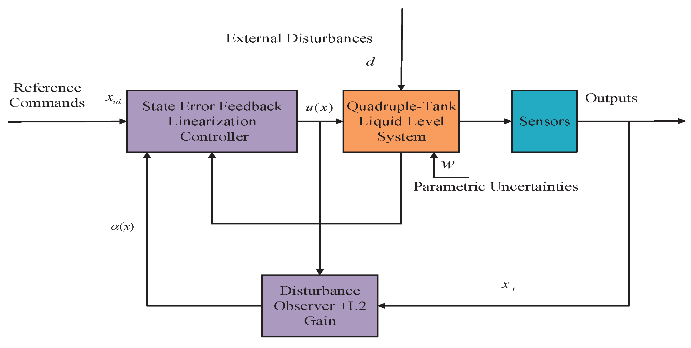
3. Control Strategy Design of the Quadruple-Tank Liquid-Level System

First of all, in view of the highly nonlinear and strong coupling characteristics of the quadruple-tank liquid-level system, without considering the uncertainty and disturbance, in an ideal state, the controller is designed with state error feedback linearization technology to realize the liquid-level position control and tracking control. Secondly, the influence of uncertain external disturbances on the quadruple-tank liquid-level system is considered. On the basis of the previous, a disturbance observer is designed to estimate the disturbance and perform disturbance compensation control. Moreover, L 2 -gain disturbance attenuation technology is employed to resolve one class of disturbance problem by uncertain parameter perturbation existing in the quadruple-tank liquid-level system. Finally, the stability of the equilibrium point of the entire system is analyzed.

3.1. The State Error Feedback Linearization Controller Design

From Equation (3), the state error feedback linearization controller u s e j is chosen as
u s e 1 u s e 2 u s e 3 u s e 4 = 1 C ( A x 1 B x 3 + v 1 ) 1 F ( D x 2 E x 4 + v 2 ) 1 H ( G x 3 + v 3 ) 1 J ( I x 4 + v 4 ) ,
u 1 u 2 = C u s e 1 + J u s e 4 F u s e 2 + H u s e 3 ,
where v i are new inputs of the equivalent linear systems [45,46,47].
With v i being the “equivalent input v” to be specified, the resulting dynamics is linear, x ˙ 1 x ˙ 2 x ˙ 3 x ˙ 4 = v 1 v 2 v 3 v 4 .
Choosing the equivalent input v i as
v 1 v 2 v 3 v 4 = x ˙ 1 d x ˙ 2 d x ˙ 3 d x ˙ 4 d + k 1 0 0 k 4 0 k 2 k 3 0 0 0 k 3 0 0 0 0 k 4 δ 1 δ 2 δ 3 δ 4 ,
where δ i = x i x i d are liquid-level tracking errors, k i are positive constants, and x i d are desired liquid-level values ( i = 1 , 2 , 3 , 4 ), the resulting closed loop dynamics is
x ˙ i + k i δ i = 0 .
This implies that δ i ( t ) 0 as t .
Analogously, provided that the desired liquid-level is a known time-varying function x i d ( t ) , the equivalent input v can be selected as
v i = x ˙ i d k i δ i ,
so as to still yield δ i ( t ) 0 as t [48].
If the desired liquid-level value x i d is a known constant, the x ˙ i d tends to zero.
Hence, the Equation (6) can be rewritten as δ ˙ 1 δ ˙ 2 δ ˙ 3 δ ˙ 4 = v 1 v 2 v 3 v 4 .
Substituting Equations (2), (4), and (6) into (5), the state error feedback linearization controller can be expressed as
u = 1 2 ( 1 + a 5 a 6 ) a 1 2 g x 1 a 3 2 g x 3 A 1 k 1 ( x 1 x 1 d ) + ( 1 + a 6 a 5 ) a 4 2 g x 4 A 4 k 4 ( x 4 x 4 d ) ( 1 + a 7 a 8 ) a 2 2 g x 2 a 4 2 g x 4 A 2 k 2 ( x 2 x 2 d ) + ( 1 + a 8 a 7 ) a 3 2 g x 3 A 3 k 3 ( x 3 x 3 d ) .
Due to
k 1 0 0 k 4 0 k 2 k 3 0 0 0 k 3 0 0 0 0 k 4 = i = 1 4 k i 0 ,
the system can be controlled.
According to the designed “ equivalent input v” and Equation (6), the desired pole of the closed-loop system is s i ( i = 1 , 2 , 3 , 4 ), and the desired closed-loop state-error system characteristic equation can be easily obtained as
( s + k 1 ) ( s + k 2 ) ( s + k 3 ) ( s + k 4 ) = 0 .
According to the requirements, the poles of four expectations on the S plane can be obtained as
s i = k i .
As k i are positive constant ( k i > 0 ), the poles to be in the left half plane.

3.2. Design of Disturbance Observer

In this paper, the quadruple-tank liquid-level system with the uncertain exogenous disturbances are considered and described as
x ˙ 1 x ˙ 2 x ˙ 3 x ˙ 4 = A x 1 + B x 4 D x 2 + E x 3 G x 3 I x 4 + C 0 0 F 0 H J 0 u 1 u 2 + d 1 d 2 d 3 d 4 ,
where d 1 , d 2 , d 3 , and d 4 are uncertain exogenous disturbances, and they are bounded. | d 1 | D 1 , | d 2 | D 2 , | d 3 | D 3 , | d 4 | D 4 , D 1 , D 2 , D 3 , and D 4 are the bounded positive constants.
The disturbance observer can be designed as
x ^ ˙ 1 x ^ ˙ 2 x ^ ˙ 3 x ^ ˙ 4 = A x ^ 1 + B x ^ 3 D x ^ 2 + E x ^ 4 G x ^ 3 I x ^ 4 + C 0 0 F 0 H J 0 u 1 u 2 + d ^ 1 d ^ 2 d ^ 3 d ^ 4 + h 1 ( x 1 x ^ 1 ) h 2 ( x 2 x ^ 2 ) h 3 ( x 3 x ^ 3 ) h 4 ( x 4 x ^ 4 ) ,
d ^ ˙ 1 d ^ ˙ 2 d ^ ˙ 3 d ^ ˙ 4 = h 5 ( x 1 x ^ 1 ) h 6 ( x 2 x ^ 2 ) h 7 ( x 3 x ^ 3 ) h 8 ( x 4 x ^ 4 ) ,
where h 1 , h 2 , h 3 , h 4 , h 5 , h 6 , h 7 , and h 8 are the adjustable parameters h 1 h 5 , h 2 h 6 , h 3 h 7 , h 4 h 8 .
With the estimated disturbances d ^ 1 , d ^ 2 , d ^ 3 , d ^ 4 and estimated states x ^ 1 , x ^ 2 , x ^ 3 , x ^ 4 , the state estimated errors and disturbance estimated errors can be expressed as
x ˜ 1 x ˜ 2 x ˜ 3 x ˜ 4 = x 1 x ^ 1 x 2 x ^ 2 x 3 x ^ 3 x 4 x ^ 4 , d ˜ 1 d ˜ 2 d ˜ 3 d ˜ 4 = d 1 d ^ 1 d 2 d ^ 2 d 3 d ^ 3 d 4 d ^ 4 .
By combining Equation (16), the first-order derivative of state estimated errors and disturbance estimated errors can be given by
x ˜ ˙ 1 x ˜ ˙ 2 x ˜ ˙ 3 x ˜ ˙ 4 = x ˙ 1 x ^ ˙ 1 x ˙ 2 x ^ ˙ 2 x ˙ 3 x ^ ˙ 3 x ˙ 4 x ^ ˙ 4 , d ˜ ˙ 1 d ˜ ˙ 2 d ˜ ˙ 3 d ˜ ˙ 4 = d ˙ 1 d ^ ˙ 1 d ˙ 2 d ^ ˙ 2 d ˙ 3 d ^ ˙ 3 d ˙ 4 d ^ ˙ 4 .
The lumped disturbances d is slowly time varying, that is, d ˙ 0 . In other words, t , d ˙ = 0 [24,48].
Hence, from Equation (17), one can acquire
d ˜ ˙ 1 d ˜ ˙ 2 d ˜ ˙ 3 d ˜ ˙ 4 = d ^ ˙ 1 d ^ ˙ 2 d ^ ˙ 3 d ^ ˙ 4 .
Substituting Equation (15) into (18), one can obtain
d ˜ ˙ 1 d ˜ ˙ 2 d ˜ ˙ 3 d ˜ ˙ 4 = h 5 x ˜ 1 h 6 x ˜ 2 h 7 x ˜ 3 h 8 x ˜ 4 .
By Equations (2), (14), and (19), the controller for the quadruple-tank liquid-level system with disturbances can be obtained as
u = 1 2 ( 1 + a 5 a 6 ) a 1 2 g x 1 a 3 2 g x 3 A 1 k 1 ( x 1 x 1 d ) A 1 h 5 d ^ 1 + ( 1 + a 6 a 5 ) a 4 2 g x 4 A 4 k 4 ( x 4 x 4 d ) A 4 h 8 d ^ 4 ( 1 + a 7 a 8 ) a 2 2 g x 2 a 4 2 g x 4 A 2 k 2 ( x 2 x 2 d ) A 2 h 6 d ^ 2 + ( 1 + a 8 a 7 ) a 3 2 g x 3 A 3 k 3 ( x 3 x 3 d ) A 3 h 7 d ^ 3 .
defining the new terms [49] as z 1 z 2 z 3 z 4 z 5 z 6 z 7 z 8 = x ˜ 1 x ˜ 2 x ˜ 3 x ˜ 4 d ˜ 1 d ˜ 2 d ˜ 3 d ˜ 4 .
Using Equations (14), (15), and (19), the first-order time derivative of the new terms can be calculated as
z ˙ 1 z ˙ 2 z ˙ 3 z ˙ 4 z ˙ 5 z ˙ 6 z ˙ 7 z ˙ 8 = h 1 0 0 0 0 0 0 0 0 h 2 0 0 0 0 0 0 0 0 h 3 0 0 0 0 0 0 0 0 h 4 0 0 0 0 h 5 0 0 0 1 0 0 0 0 h 6 0 0 0 1 0 0 0 0 h 7 0 0 0 1 0 0 0 0 h 8 0 0 0 1 z 1 z 2 z 3 z 4 z 5 z 6 z 7 z 8 ,
with
M = h 1 0 0 0 0 0 0 0 0 h 2 0 0 0 0 0 0 0 0 h 3 0 0 0 0 0 0 0 0 h 4 0 0 0 0 h 5 0 0 0 1 0 0 0 0 h 6 0 0 0 1 0 0 0 0 h 7 0 0 0 1 0 0 0 0 h 8 0 0 0 1 .
Utilizing Equation (22), Equation (21) can be shortened to
z ˙ i = M i z i .
Due to h 1 h 5 , h 2 h 6 , h 3 h 7 , h 4 h 8 , we can get
M = h 1 0 0 0 0 0 0 0 0 h 2 0 0 0 0 0 0 0 0 h 3 0 0 0 0 0 0 0 0 h 4 0 0 0 0 h 5 0 0 0 1 0 0 0 0 h 6 0 0 0 1 0 0 0 0 h 7 0 0 0 1 0 0 0 0 h 8 0 0 0 1 0 .
Remark: By choosing appropriate h i , it is easy to prove that the system is stable. It can be seen from Equation (24) that the eigenvalues of M are in the left half open plane of the complex plane, so the equilibrium point of the nonlinear system is asymptotically stable [49].

3.3. L 2 -Gain Disturbance Attenuation Law Injection

Considering a class of nonlinear systems with disturbances, system (13) can be rephrased as
x ˙ = f ( x ) + g ( x ) u + d + w ,
where, x = x 1 x 2 x 3 x 4 T , w is a disturbance with uncertain parameter perturbation.
Combining Equations (13) and (25), the quadruple-tank liquid-level system can be rewritten as
x ˙ 1 x ˙ 2 x ˙ 3 x ˙ 4 = A x 1 + B x 3 D x 2 + E x 4 G x 3 I x 4 f ( x ) + C 0 0 F 0 H J 0 g ( x ) u 1 u 2 + d 1 d 2 d 3 d 4 d + w 1 w 2 w 3 w 4 w .
Penalty signal is defined for system (25) as follows:
φ = l ( x ) g ( x ) N ( δ ) δ ,
where l ( x ) is a weighted matrix and N ( δ ) = k i 2 δ 2 .
Consider a system (25) with a penalty signal (27). For any given γ > 0 , the goal of L 2 attenuating perturbation interference is achieved through the following feedback control law. Find a control law α ( x ) and a positive storage function N ( δ ) such that the γ -dissipation inequality (28)
N ˙ ( δ ) + Q ( x ) 1 2 ( γ 2 w 2 φ 2 ) ,
where Q ( x ) is a non-negative definite function. This means that N ( δ ) serves as the storage function for the closed loop system.
In view of system (25) and penalty signal (27), for any given positive γ , the L 2 disturbance attenuation goal will be realized by the state error feedback
α ( x ) = 1 2 1 γ 2 I + l ( x ) g T ( x ) N ( δ ) δ .
In conclusion, the composited controller can be designed as
u = 1 2 ( 1 + a 5 a 6 ) a 1 2 g x 1 a 3 2 g x 3 A 1 k 1 ( x 1 x 1 d ) + A 1 x ˙ 1 d A 1 h 5 d ^ 1 + ( 1 + a 6 a 5 ) a 4 2 g x 4 A 4 k 4 ( x 4 x 4 d ) + A 4 x ˙ 4 d A 4 h 8 d ^ 4 ( 1 γ 2 + 1 ) a 6 a 5 + a 6 · k 1 A 1 ( x 1 x 1 d ) + a 5 a 5 + a 6 · k 4 A 4 ( x 4 x 4 d ) ( 1 + a 7 a 8 ) a 2 2 g x 2 a 4 2 g x 4 A 2 k 2 ( x 2 x 2 d ) + A 2 x ˙ 2 d A 2 h 6 d ^ 2 + ( 1 + a 8 a 7 ) a 3 2 g x 3 A 3 k 3 ( x 3 x 3 d ) + A 3 x ˙ 3 d A 3 h 7 d ^ 3 ( 1 γ 2 + 1 ) a 8 a 7 + a 8 · k 2 A 2 ( x 2 x 2 d ) + a 7 a 7 + a 8 · k 3 A 3 ( x 3 x 3 d ) .

3.4. Asymptotic Stability Analysis

Choose a Lyapunov function for the quadruple-tank liquid-level system (26) as
V = 1 2 i = 1 4 δ i 2 .
Then, the first-order time derivative of the selected Lyapunov function (31) can be calculated as
V ˙ = i = 1 4 δ i δ ˙ i .
By combining Equations (6) and (8), the first-order time derivative of the selected Lyapunov function can be expressed as
V ˙ = i = 1 4 k i δ i 2 < 0 .
Obviously, V is positive definite and V ˙ is negative definite, satisfying the Lyapunov stability theorem, so the desired equilibrium point x i d is asymptotically stable [50,51,52,53].

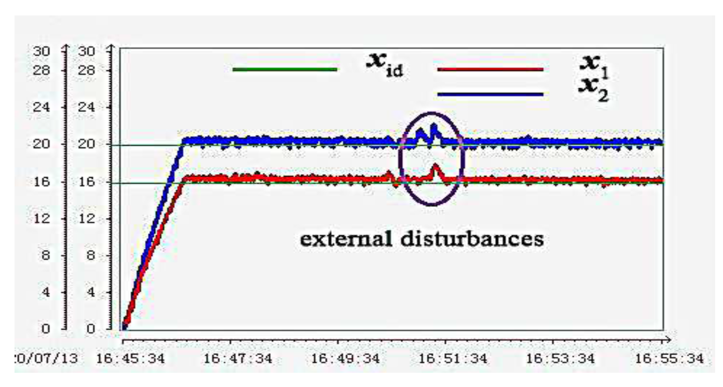
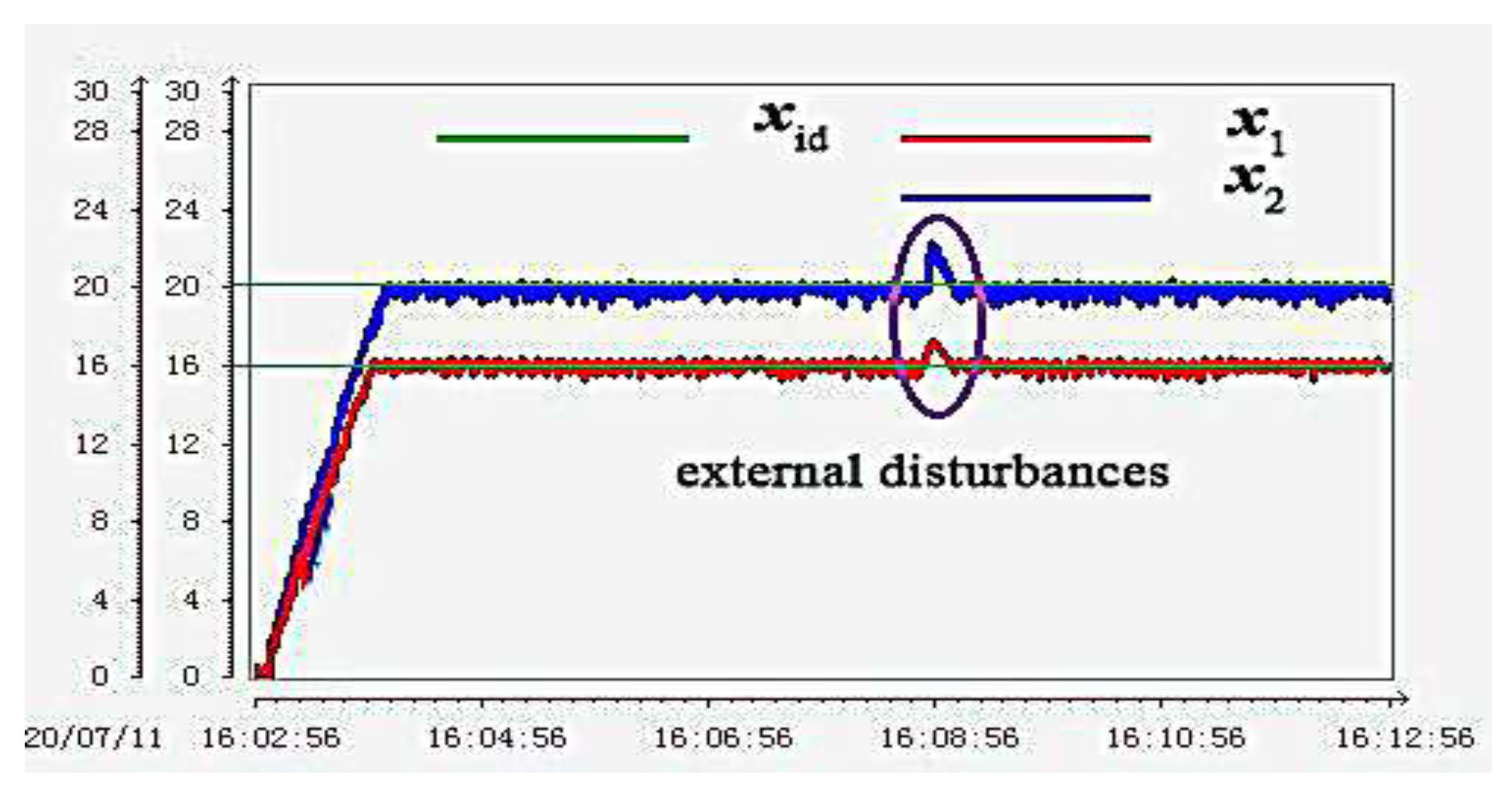
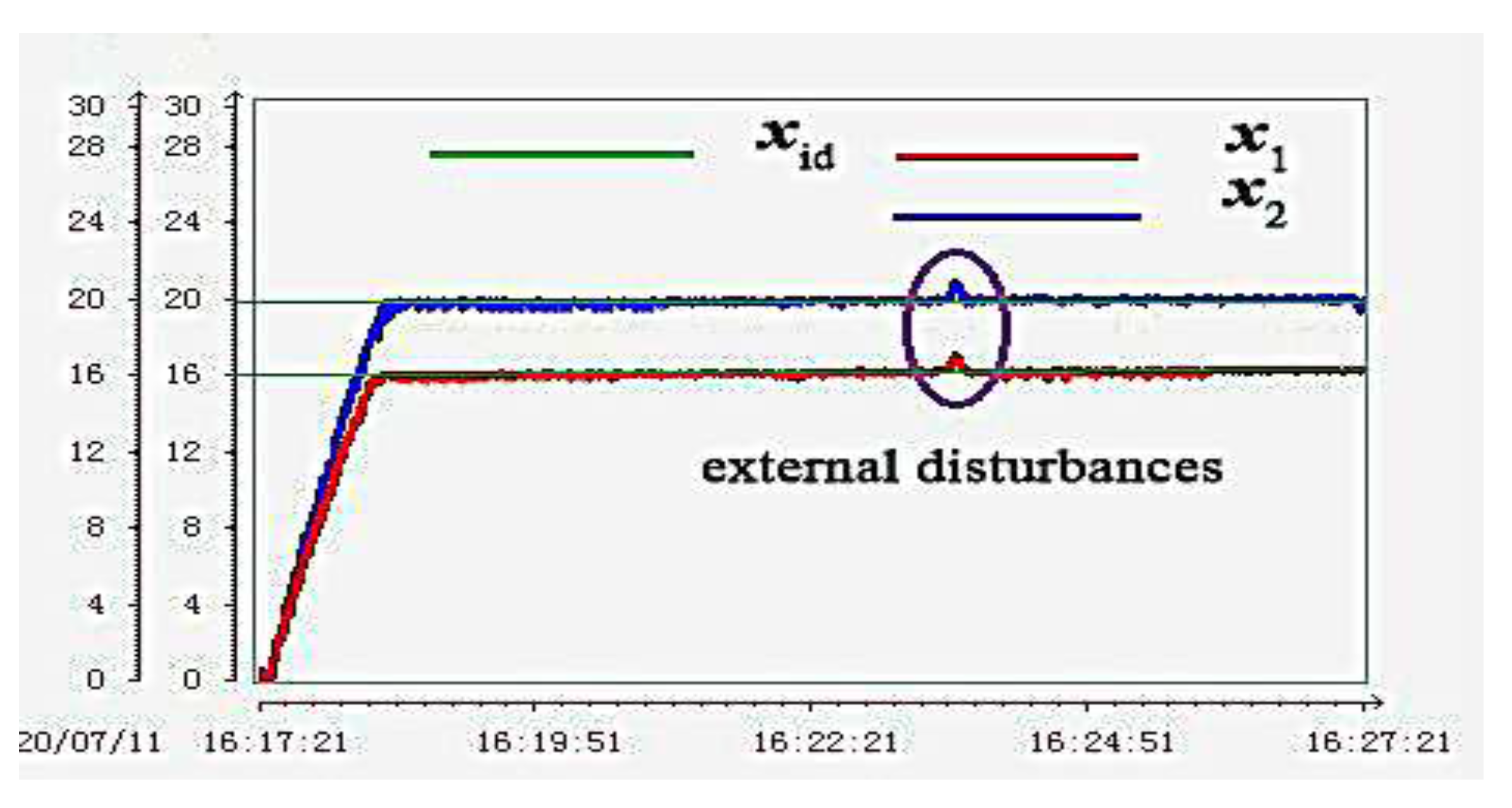
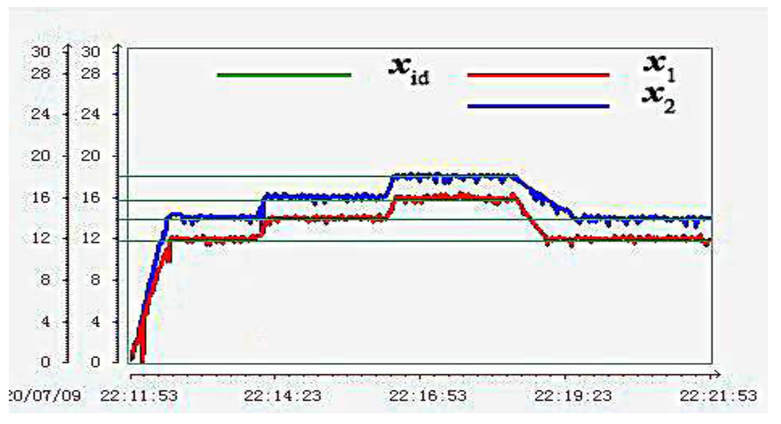
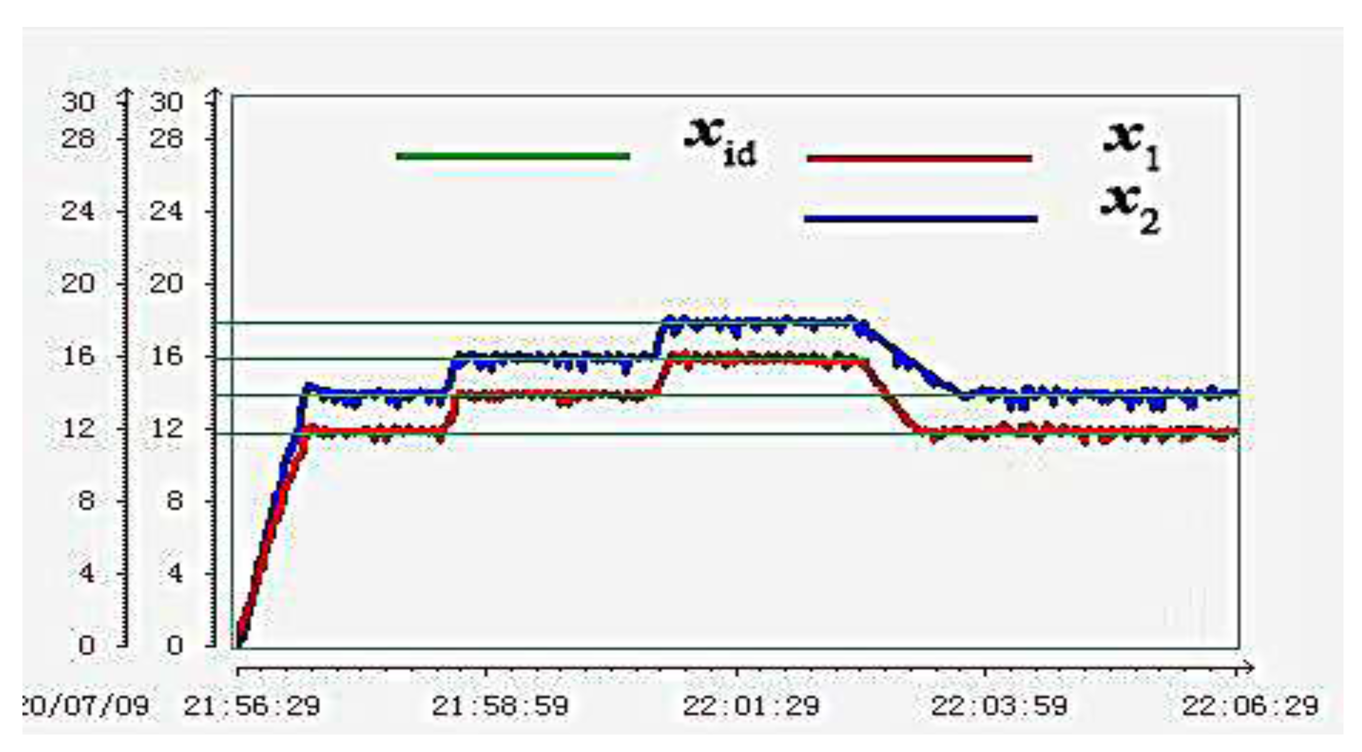
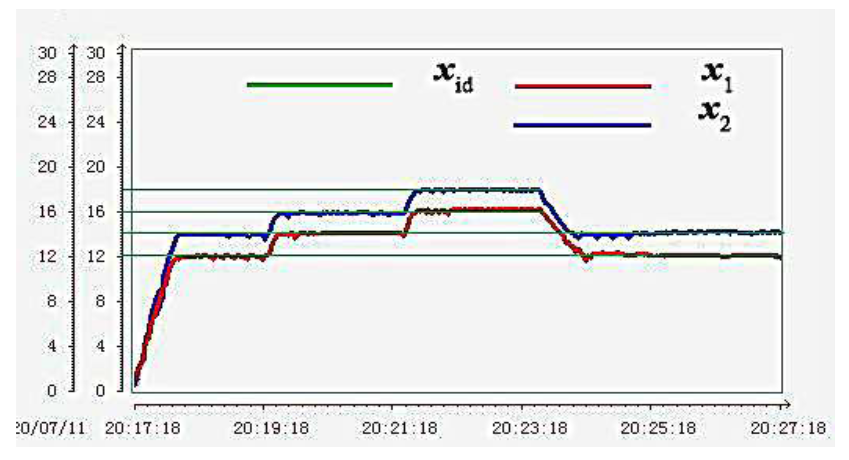
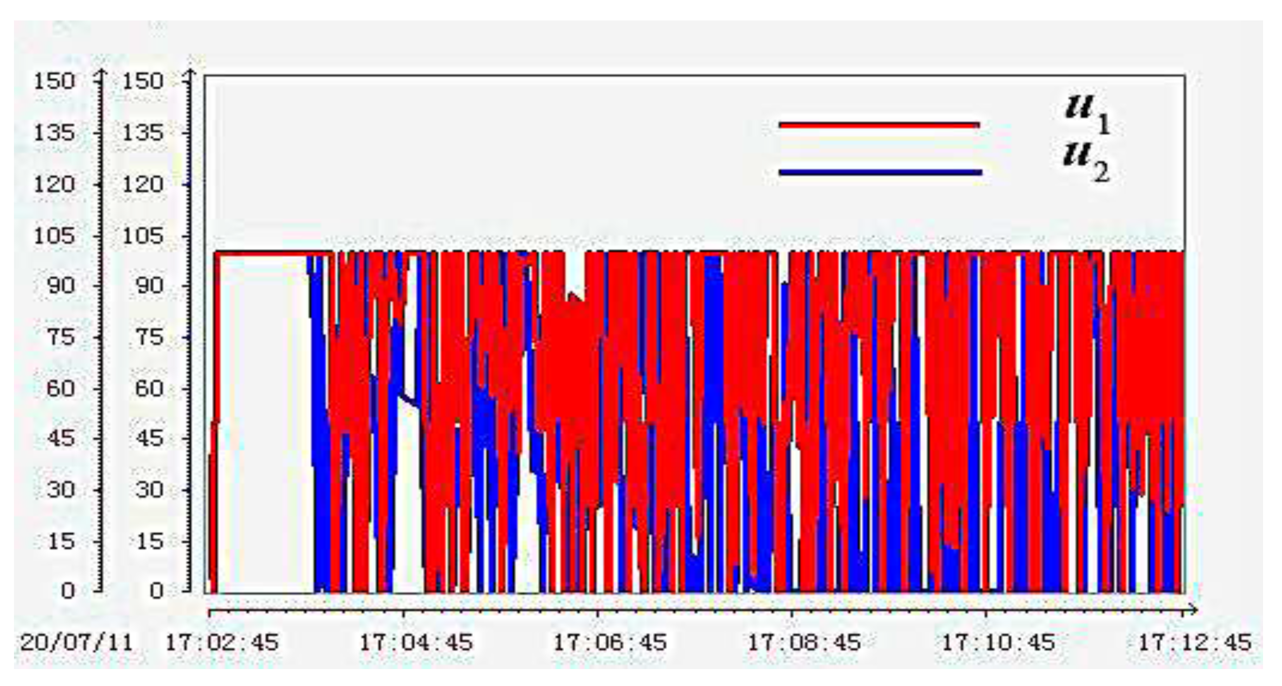
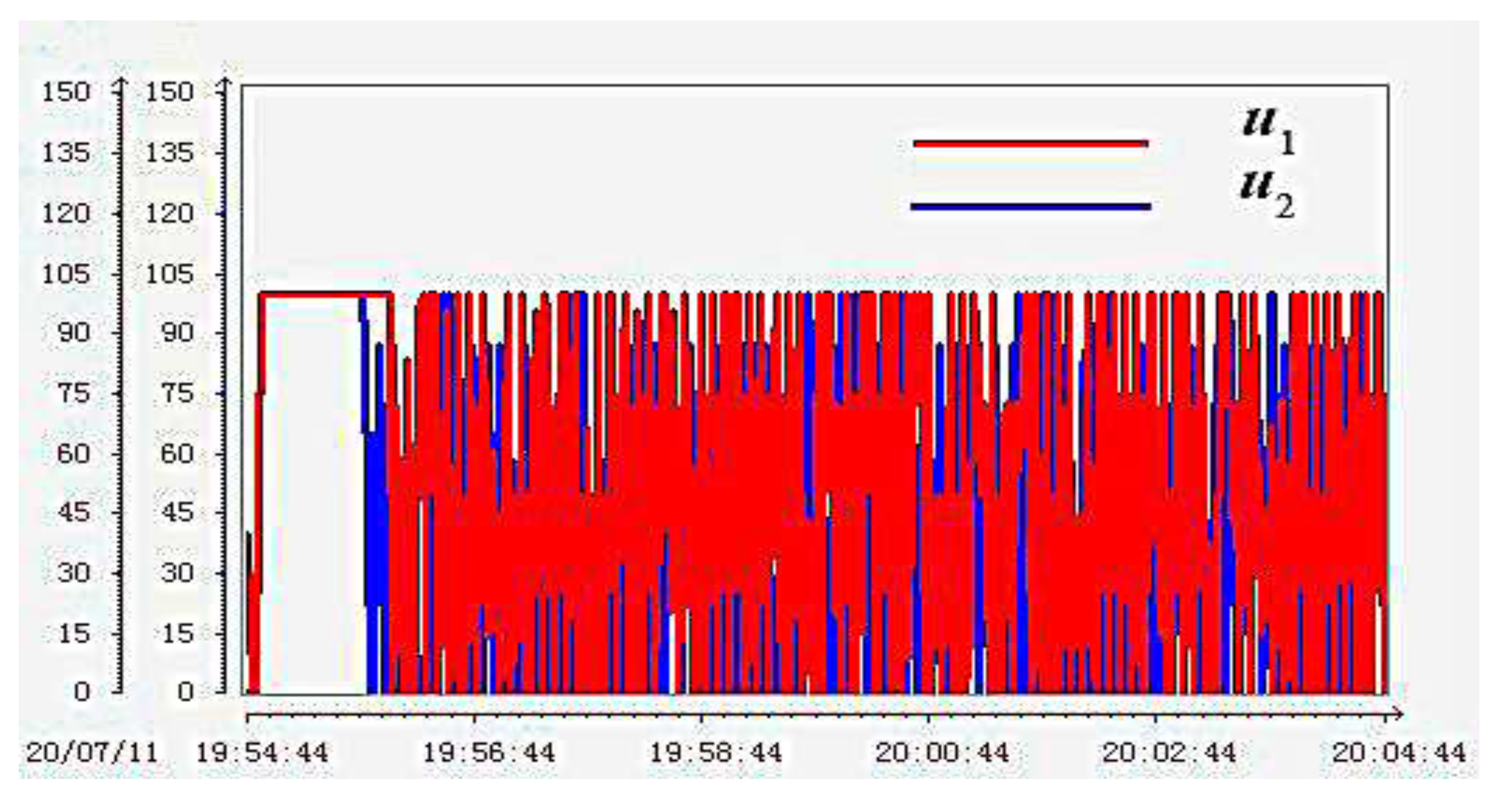
4. Experiment Results and Analysis

The experimental device of quadruple-tank liquid-level system is a typical process control object. The device uses an ultrasonic sensor to detect the liquid-level value, a direct current (DC) water pump as an actuator, and a Siemens S7-300 series programmable logic controller (PLC) with its special analog input (AI) and special analog output (AO) modules to build a local closed-loop control system. At the same time, the communication connection between MATLAB/Simulink and PLC is established using Object Linking and Embedding for Process Control (OPC) technology. In PLC part, CPU S7-300 module of Siemens is selected, the special AI module is extended to collect the actual liquid-level values of four tanks, and the AO module is extended to provide the actual required analog voltage value of the pumps. Matlab and PLC/HMI (Human Machine Interface) industrial Control system are integrated through OPC communication technology. The experimenter completed the controller design and real-time Control under the environment of Matlab/Simulink. That is, through OPC communication, PLC data and events can be monitored, invoked, and processed on a personal computer (PC).
The driver of the water pump has a double closed loop adjustment function, and the speed adjustment method adopted by this device is 1–5 V analog speed adjustment, for which the corresponding analog digital signal range is 0–100. Considering that input saturation may occur in the start-up and operation stage of the experimental system, we add a limiter to the output end of the controller to ensure the normal operation of the system and reduce the impact of input exceeding the limit on the system. As shown in Figure 3, SIMATIC Windows Control Center (WinCC) of Siemens is used as the upper computer state monitoring software in this system. WinCC is a process visualization system that can effectively control automated processes. It can be easily combined with standard and user programs to establish human–machine interface and accurately meet actual needs. The PLC adopts the industrial Ethernet communication method and connects a network cable to the computer through the PROFINET interface. This computer is used as the upper computer. The above software is installed, and the compiled program is downloaded to the central processing unit (CPU) of PLC. The system establishes communication, so that the collected real-time liquid-level value and the control quantity for the pump can be embedded in the Simulink environment, and finally, a closed-loop feedback system for liquid-level control is constructed on Simulink.
Before powering on, turn on the air switch of the PLC system on the back panel of the device. The CPU status indicator of the PLC starts to flash. Wait for a while. When only the DC5V and RUN indicator lights are green, it means the system is operating normally. When the line is connected incorrectly or there is a problem with the module, the corresponding indicator will be red to show a warning. At this time, we need to turn off the main switch and seek professional personnel to check the line and module. After the above operations are completed, we must first open the computer’s upper WinCC, it is the server because it can be opened to ensure that the relevant data can be read and written normally in the Matlab environment, and then the relevant experiments can be performed on the Matlab.
The parameters of the quadruple-tank liquid-level system mode are shown as Table 1.
In order to verify the superiority of the above control strategy and the effectiveness of the results, the classical PID and sliding mode control methods are compared.
Then, the classic PID control law [5,6,7] can be described as
u P I D = k p 1 ( x 1 x 1 d + x 4 x 4 d ) + k i 1 ( x 1 x 1 d + x 4 x 4 d ) d t + k d 1 ( x ˙ 1 x ˙ 1 d + x ˙ 4 x ˙ 4 d ) k p 2 ( x 2 x 2 d + x 3 x 3 d ) + k i 2 ( x 2 x 2 d + x 3 x 3 d ) d t + k d 2 ( x ˙ 2 x ˙ 2 d + x ˙ 3 x ˙ 3 d ) ,
where k p 1 , k p 2 , k i 1 , k i 2 , k d 1 , and k d 2 are positive constants
The sliding mode surface η is designed as
η 1 = ( δ 1 + δ 4 ) + c 1 ( δ 1 + δ 4 ) d t η 2 = ( δ 2 + δ 3 ) + c 2 ( δ 2 + δ 3 ) d t .
In order to achieve good performance, such as fast convergence and better tracking precision, the sliding mode approach law can be chosen as follows:
η ˙ 1 = m 1 sgn ( η 1 ) n 1 η 1 η ˙ 2 = m 2 sgn ( η 2 ) n 2 η 2 .
Substituting Equations (35) and (36) into (1), sliding mode controller can be calculated as
u S M C = A 1 2 x ˙ 1 d + x ˙ 4 d + a 1 A 1 2 g x 1 a 3 A 1 2 g x 3 + a 4 A 4 2 g x 4 m 1 sgn ( η 1 ) ( n 1 + c 1 ) ( x 1 x 1 d + x 4 x 4 d ) n 1 c 1 ( x 1 x 1 d + x 4 x 4 d ) d t A 2 2 x ˙ 2 d + x ˙ 3 d + a 2 A 2 2 g x 2 a 4 A 2 2 g x 4 + a 3 A 3 2 g x 3 m 2 sgn ( η 2 ) ( n 2 + c 2 ) ( x 2 x 2 d + x 3 x 3 d ) n 2 c 2 ( x 2 x 2 d + x 3 x 3 d ) d t ,
where c 1 , c 2 , m 1 , m 2 , n 1 , and n 2 are positive constants.
In this paper, the external disturbances of Tank 1 and Tank 2 are given in the form of additional water injection. The schematic of the proposed control strategy and the device control principle diagram are shown in Figure 4 and Figure 5, respectively. The desired equilibrium points are x 1 = 16 cm, x 2 = 20 cm. In the experimental research, the PID parameters, the sliding mode controller parameters, and the proposed composite controller parameters are given in Table 2, Table 3 and Table 4, respectively. For the determination and optimization of the parameters, the Lyapunov stability theorem is used to determine the range of parameters, and then the specific parameter values are determined by the empirical trial and error method.
Due to the PLC system loaded in this experimental device, only one system can be used for each experiment, and the switch between the two can only be realized by the empty space on the back plate. So, the experimental results can only be displayed and saved in the form of interception of the WinCC monitoring interface because of limitations of the experimental equipment. In the experimental results, the red curve is the liquid-level curve of Tank 1, the blue curve is the liquid-level curve of Tank 2, and the green curve is the reference liquid-level curve.
As show in Figure 6, Figure 7 and Figure 8, the obvious fluctuation occurs in the liquid-level curves of the classical PID control algorithm, the steady-state error value is larger, and the steady-state error value is e s s ( ) = ± 0.6 cm. Compared with PID control algorithm, the liquid-level curves steady-state error value is smaller using the traditional sliding mode control method, and the steady-state error value is e s s ( ) = ± 0.4 cm, but there is a high frequency of fluctuation. The liquid-level curves of the purposed control strategy have no obvious fluctuation, and the steady-state error value is smaller than the above methods—the steady-state error value is e s s ( ) = ± 0.1 cm. When a certain amount of water is injected into Tanks 1 and 2, the proposed control strategy has a smaller fluctuation range than the previous two control methods, the fluctuation ranges are 0.5 cm, 1.5 cm, and 1.5 cm. It can be easily seen from the figure that when the system injects external disturbances, the liquid-level curves under the three control strategies have obvious fluctuations, but the control strategy proposed in this paper has smaller fluctuations. Moreover, it can quickly return to the steady-state expected value, with an adjusted time of t s = 15 s. From Figure 6, Figure 7 and Figure 8 and the calculated performance indicators, it can be concluded that the proposed control method in this article has higher control accuracy and better stability for position control.
Figure 9, Figure 10 and Figure 11 show that the liquid-level tracking of two rises and one drop is realized after starting and reaching the stable equilibrium point. While the classical PID algorithm and the traditional sliding mode control method of liquid-level curves can reach a certain amount of tracking effect, there are still obvious fluctuations and larger steady-state error. The steady-state errors are e s s ( ) = ± 0.5 cm and e s s ( ) = ± 0.3 cm. Through the proposed control strategy in this paper, liquid-level curves not only achieve a better tracking performance, but also have a very small steady-state error—the steady-state error value is e s s ( ) = ± 0.05 cm. Moreover, the level curves of PID and SMC methods have overshoots σ % in the first stage of tracking control. The overshoots of the two levels of the two methods are σ 1 % = 3.8 % , σ 2 % = 3.0 % , σ 1 % = 3.1 % , and σ 2 % = 2.5 % . However, the proposed method in this paper has no overshoot phenomenon.
From Figure 12, Figure 13 and Figure 14, the control input curves of classical PID algorithm and traditional sliding mode control method are frequently switched between 0 and 100, and the fluctuation range of the control input curves based on the controller proposed in this paper is 0–30, which is only 30% of the above methods. The control input curves of classical PID algorithm and traditional sliding mode control method frequently reached the upper limit of control input, which will seriously affect the service life of the equipment. In summary, compared with the other two methods, the control strategy proposed in this paper has higher accuracy of liquid-level position control; higher fitting degree of tracking control; efficient disturbance suppression performance; and more importantly, the output of the controller is more stable. Therefore, the advantages of the proposed method in industrial practice are more prominent.

5. Conclusions

This paper has developed a fresh state error feedback linearization control strategy with DOB and L 2 for a quadruple-tank liquid-level system. In the first place, the state error feedback linearization technique is employed to design the controller to achieve liquid-level position control and tracking control. In the next place, DOB is purposed to estimate uncertain exogenous disturbances and applied to compensation control. Then, the L 2 -gain disturbance attenuation technology is designed to resolve one class of disturbance problem by uncertain parameter perturbation existing in the quadruple-tank liquid-level system. In conclusion, the extensive experimental results validate the effectiveness of the developed control scheme compared with classical PID and the SMC strategies, such that the position control and tracking control error of the liquid level is smaller, the fluctuation caused by external disturbance is smaller, there is no frequent fluctuation caused by the parameter uncertainty perturbation, and the control output of the actual controller is smaller and more stable. In addition, compared with some of the literatures listed in the introduction, the proposed control strategy still has outstanding effects in the aspects of liquid-level position control, tracking control, uncertain exogenous disturbances rejection, and disturbances by uncertain parameter perturbation restraining in this paper. Moreover, a large number of experimental verifications further confirmed the broad application of this proposed strategy in the field of industrial process control.

Author Contributions

X.M.; developing the theoretical results, writing the paper, and performing the experiments; H.Y.; revising the mathematical formulations; T.X., analyzing the algorithms; H.W.; ensuring the hardware and software support. All authors have read and agreed to the published version of the manuscript.

Funding

This research was funded by National Natural Science Foundation of China, grant number 61573203.

Conflicts of Interest

The authors declare no conflict of interest.

Nomenclature

D O B disturbance observer
P I D proportion integration differentiation
S M C sliding mode control
M I M O multi-input and multioutput
D O F degree of freedom
P I proportion integral
L C L inductance capacitance inductance
A D R C active disturbance rejection controller
S I S O single input single output
D C direct current
P L C programmable logic controller
P C personal computer
A I analog input
A O analog output
O P C object linking and embedding for process control
C P U central processing unit
W i n C C windows control center
x i the height of liquid inside the tank i
x i d desired liquid-level value
A i the cross-section of tank i
a i the cross-section of the outlet manual valve i
gthe gravitational acceleration
t r rise time
e s s steady-state error
t s adjusting time
σ % overshoots

References

  1. Johansson, K.H. The Quadruple-Tank Process: A Multivariable Laboratory Process with an Adjustable Zero. IEEE Trans. Control. Syst. Technol. 2000, 8, 456–465. [Google Scholar]
  2. Gatzke, E.P.; Meadows, E.S.; Wang, C.; Doyle, F.J. Model based control of a four-tank system. Comput. Chem. Eng. 2000, 24, 1503–1509. [Google Scholar]
  3. Shneiderman, D.; Palmor, Z.J. Properties and control of the quadruple-tank process with multivariable dead-times. J. Process Control 2010, 20, 18–28. [Google Scholar]
  4. Vadigepalli, R.; Gatzke, E.P.; Doyle, F.J. Robust Control of a Multivariable Experimental Four-Tank System. Ind. Eng. Chem. Res. 2001, 40, 1916–1927. [Google Scholar]
  5. Kumar, E.; Mithunchakravarthi, B.; Dhivya, N. Enhancement of PID controller performance for a quadruple tank process with minimum and non-minimum phase behaviors. IEEE Trans. Control. Syst. Technol. 2005, 13, 480–489. [Google Scholar]
  6. Ang, K.H.; Chong, G.; Li, Y. PID control system analysis, design and technology. IEEE Trans. Control Syst. Technol. 2005, 13, 559–576. [Google Scholar]
  7. Holic, I.; Vesely, V. Robust PID controller design for coupled-tank process using Labreg software. IFAC Proc. 2012, 45, 442–447. [Google Scholar]
  8. Kumar, K.; Patwardhan, S.C.; Noronha, S. Development of an adaptive and explicit dual model predictive controller based on generalized orthogonal basis filters. J. Process Control 2019, 93, 196–214. [Google Scholar]
  9. Yu, T.Y.; Zhao, J.; Xu, Z.H.; Chen, X.; Biegler, L.T. Sensitivity-based hierarchical distributed model predictive control of nonlinear processes. J. Process Control 2019, 84, 146–167. [Google Scholar]
  10. Thamallah, A.; Sakly, A.; M’Sahli, F. A new constrained PSO for fuzzy predictive control of Quadruple-Tank process. Measurement 2019, 136, 93–104. [Google Scholar]
  11. Pan, H.Z.; Wong, H.; Kapila, V.; Queiroz, M.S.D. Experimental validation of a nonlinear backstepping liquid level controller for a state coupled two tank system. Control Eng. Pract. 2015, 13, 27–40. [Google Scholar] [CrossRef]
  12. Meng, X.X.; Yu, H.S.; Wu, H.R.; Xu, T. Disturbance Observer-Based Integral Backstepping Control for a Two-Tank Liquid Level System Subject to External Disturbances. Math. Probl. Eng. 2020, 3, 1–22. [Google Scholar]
  13. Shah, D.H.; Patel, D.M. Design of sliding mode control for quadruple-tank MIMO process with time delay compensation. J. Process Control 2019, 76, 46–61. [Google Scholar] [CrossRef]
  14. Chaudhari, V.; Tamhane, B.; Kurode, S. Robust Liquid Level Control of Quadruple Tank System-Second Order Sliding Mode Approach. IFAC Pap. Online 2020, 53, 7–12. [Google Scholar]
  15. Yu, H.S.; Yu, J.P.; Wu, H.R.; Li, H.L. Energy-shaping and integral control of the three-tank liquid level system. Nonlinear Dyn. 2013, 73, 2149–2156. [Google Scholar] [CrossRef]
  16. Mahapatro, S.R.; Subudhi, B.; Ghosh, S. Design and experimental realization of a robust decentralized PI controller for a coupled tank system. ISA Trans. 2019, 89, 158–168. [Google Scholar]
  17. Silva, F.F.A.; Adorno, B.V. Whole-body Control of a Mobile Manipulator Using Feedback Linearization and Dual Quaternion Algebra. J. Intell. Robot. Syst. 2018, 91, 249–262. [Google Scholar] [CrossRef] [Green Version]
  18. Bahmani, E.; Rahmani, M. An LMI approach to dissipativity-based control of nonlinear systems. J. Frankl. Inst. 2020, 357, 5699–5719. [Google Scholar] [CrossRef]
  19. Pradhan, J.K.; Ghosh, A.; Bhende, C.N. Two-degree-of-freedom multi-input multi-output proportional–integral–derivative control design: Application to quadruple-tank system. Appl. Soft Comput. 2020, 96, 1–17. [Google Scholar]
  20. Accetta, A.; Alonge, F.; Cirrincione, M.; D’Ippolito, F.; Pucci, M.; Rabbeni, R.; Sferlazza, A. Robust Control for High Performance Induction Motor Drives Based on Partial State-Feedback Linearization. IEEE Trans. Ind. Appl. 2019, 55, 490–503. [Google Scholar]
  21. Martinez-Trevi∼no, B.A.; Aroudi, A.E.; Cid-Pastor, A.; Martinez-Salamero, L. Nonlinear Control for Output Voltage Regulation of a Boost Converter With a Constant Power Load. IEEE Trans. Power Electron. 2019, 34, 10381–10385. [Google Scholar]
  22. Yang, S.F.; Wang, P.; Tang, Y. Feedback Linearization-Based Current Control Strategy for Modular Multilevel Converters. IEEE Trans. Power Electron. 2018, 33, 161–174. [Google Scholar]
  23. Li, S.; Ahn, C.K.; Xiang, Z.R. Decentralized Stabilization for Switched Large-Scale Nonlinear Systems via Sampled-Data Output Feedback. IEEE Syst. J. 2018, 13, 4335–4343. [Google Scholar] [CrossRef]
  24. Pourasghar, M.; Puig, V.; Ocampo-Martinez, C. Interval observer-based fault detectability analysis using mixed set-invariance theory and sensitivity analysis approach. Int. J. Syst. Sci. 2019, 50, 495–516. [Google Scholar] [CrossRef]
  25. Al-Durra, A.; Errouissi, R. Robust Feedback-Linearization Technique for Grid-tied LCL Filter Systems Using Disturbance Estimation. IEEE Trans. Ind. Appl. 2019, 55, 3185–3197. [Google Scholar]
  26. Chen, W.H. Disturbance Observer Based Control for Nonlinear Systems. IEEE Trans. Mechatron. 2004, 9, 706–710. [Google Scholar]
  27. Yang, Z.J.; Sugiura, H. Robust nonlinear control of a three-tank system using finite-time disturbance observers. Control Eng. Pract. 2019, 84, 63–71. [Google Scholar] [CrossRef]
  28. Gouta, H.; Said, S.H.; Turki, A.; M’Sahli, F. Experimental sensorless control for a coupled two-tank system using high gain adaptive observer and nonlinear generalized predictive strategy. ISA Trans. 2019, 87, 187–199. [Google Scholar] [CrossRef]
  29. Chen, W.H.; Yang, J.; Guo, L.; Li, S.H. Disturbance-Observer-Based Control and Related Methods-An Overview. IEEE Trans. Ind. Electron. 2016, 63, 1083–1095. [Google Scholar] [CrossRef] [Green Version]
  30. Varshney, D.; Bhushan, M.; Patwardhan, S.C. Patwardhan. State and parameter estimation using extended Kitanidis Kalman filter. J. Process Control 2019, 76, 98–111. [Google Scholar]
  31. Huang, C.Z.; Canuto, E.; Novara, C. The four-tank control problem: Comparison of two disturbance rejection control solutions. ISA Trans. 2017, 71, 252–271. [Google Scholar] [CrossRef] [PubMed] [Green Version]
  32. Adaily, S.; Mbarek, A.; Garna, T.; Ragot, J. Optimal Multimodel Representation by Laguerre Filters Applied to a Communicating Two Tank System. J. Syst. Sci. Complexitys 2018, 31, 621–646. [Google Scholar]
  33. Yu, H.S.; Yu, J.P.; Liu, J.; Song, Q. Nonlinear control of induction motors based on state error PCH and energyshaping principle. Nonlinear Dyn. 2013, 72, 49–59. [Google Scholar] [CrossRef]
  34. Xu, T.; Yu, H.S.; Yu, J.P.; Meng, X.X. Adaptive Disturbance Attenuation Control of Two Tank Liquid Level System With Uncertain Parameters Based on Port-Controlled Hamiltonian. IEEE Access 2020, 8, 47384–47392. [Google Scholar] [CrossRef]
  35. Meng, X.X.; Yu, H.S.; Xu, T.; Wu, H.R. Sliding mode disturbance observer-based the port-controlled Hamiltonian control for a four-tank liquid level system subject to external disturbances. In Proceedings of the 2020 Chinese Control And Decision Conference (CCDC), Hefei, China, 23–25 August 2020; pp. 1720–1725. [Google Scholar]
  36. Cao, J.D.; Manivannan, R.; Chong, K.; Lv, X.X. Enhanced L2 - L state estimation design for delayed neural networks including leakage term via quadratic-type generalized free-matrix-based integral inequality. J. Frankl. Inst. 2019, 356, 7371–7392. [Google Scholar] [CrossRef]
  37. Canuto, E.; Acua-Bravo, W.; Agostani, M.; Bonadei, M. Digital current regulator for proportional electro-hydraulic valves with unknown disturbance rejection. ISA Trans. 2014, 53, 909–919. [Google Scholar] [CrossRef]
  38. Trierweiler, J.O.; Francisco, D.D.O.V.; Botelho, R.; Farenzena, M. Channel oriented approach for multivariable model updating using historical data. Comput. Chem. Eng. 2020, 143, 1–13. [Google Scholar] [CrossRef]
  39. Nguyen, T.S.; Hoang, N.H.; Hussain, M.A.; Tan, C.K. Tracking-error control via the relaxing port-Hamiltonian formulation: Application to level control and batch polymerization reactor. J. Process Control 2019, 80, 152–166. [Google Scholar] [CrossRef]
  40. Meng, X.X.; Yu, H.S.; Wu, H.R.; Xu, T. Research on the smooth switching control strategy for the four-tank liquid level system. In Proceedings of the 2019 Chinese Automation Congress (CAC), Hangzhou, China, 22–24 November 2019; pp. 5187–5193. [Google Scholar]
  41. Pourasghar, M.; Combastel, C.; Puig, V.; Ocampo-Martinez, C. FD-ZKF: A Zonotopic Kalman Filter optimizing fault detection rather than state estimation. J. Process Control 2019, 73, 89–102. [Google Scholar] [CrossRef] [Green Version]
  42. Patel, H.R.; Shah, V.A. Stable Fault Tolerant Controller Design for Takagi–Sugeno Fuzzy Model-Based Control Systems via Linear Matrix Inequalities: Three Conical Tank Case Study. Energies 2019, 12, 2221. [Google Scholar] [CrossRef] [Green Version]
  43. Mystkowski, A.; Kierdelewicz, A. Fractional-Order Water Level Control Based on PLC: Hardware-In-The-Loop Simulation and Experimental Validation. Energies 2018, 11, 2928. [Google Scholar] [CrossRef] [Green Version]
  44. Radac, M.B.; Precup, R.E. Data-Driven Model-Free Tracking Reinforcement Learning Control with VRFT-based Adaptive Actor-Critic. Appl. Sci. 2019, 9, 1807. [Google Scholar] [CrossRef] [Green Version]
  45. Wu, Y.Q.; Isidori, A.; Lu, R.; Khalil, H.K. Performance Recovery of Dynamic Feedback-Linearization Methods for Multivariable Nonlinear Systems. IEEE Trans. Autom. Control. 2020, 65, 1365–1380. [Google Scholar] [CrossRef]
  46. Djilal, L.; Sanchez, E.N.; Belkheiri, M. Real-time Neural Input–Output Feedback Linearization control of DFIG based wind turbines in presence of grid disturbances. Control Eng. Pract. 2019, 83, 151–164. [Google Scholar] [CrossRef]
  47. Hesar, H.M.; Zarchi, H.A.; Khoshhava, M.A. Online maximum torque per ampere control for induction motor drives considering iron loss using input–output feedback linearization. IET Electr. Power Appl. 2019, 13, 2113–2120. [Google Scholar] [CrossRef]
  48. Fu, B.Z.; Wang, Q.Z.; He, W. Nonlinear Disturbance Observer-Based Control for a Class of Port-Controlled Hamiltonian Disturbed Systems. IEEE Access 2018, 6, 50299–50305. [Google Scholar] [CrossRef]
  49. Slotine, J.-J.E.; Li, W. Lyapunov’s theoretical basis. In Applied Nonlinear Control; Jennifer Wenzel, F., Karen Stephens, A., Eds.; Slotine Massachusetts Institute of Technolog: Prentice Hall Englewood Cliffs, NJ, USA, 1991; pp. 53–55. [Google Scholar]
  50. Yang, L.Y.; Feng, C.C.; Liu, J.H. Control Design of LCL Type Grid-Connected Inverter Based on State Feedback Linearization. Electronics 2019, 8, 877. [Google Scholar] [CrossRef] [Green Version]
  51. Mahmud, M.A.; Roy, T.K.; Saha, S.; Haque, E.M.; Pota, H.R. Robust Nonlinear Adaptive Feedback Linearizing Decentralized Controller Design for Islanded DC Microgrids. IEEE Trans. Ind. Appl. 2019, 55, 5343–5352. [Google Scholar] [CrossRef]
  52. Preininger, J.; Scarinci, T.; Veliov, V.M. Metric Regularity Properties in Bang-Bang Type Linear-Quadratic Optimal Control Problems. Set-Valued Var. Anal. 2019, 27, 381–404. [Google Scholar] [CrossRef]
  53. Dontchev, A.L.; Hager, W.W. Lipschitzian stability in nonlinear control and optimization. SIAM J. Control. Optim. 2019, 31, 569–603. [Google Scholar] [CrossRef]
Figure 1. The quadruple-tank liquid-level system experimental equipment.
Energies 13 05500 g001
Figure 2. The schematic diagram of the quadruple-tank structure.
Energies 13 05500 g002
Figure 3. Monitoring system of networked four-tank experiment platform.
Energies 13 05500 g003
Figure 4. The schematic of the proposed control strategy.
Energies 13 05500 g004
Figure 5. Device control principle diagram. WinCC—Windows Control Center; PLC—programmable logic controller.
Energies 13 05500 g005
Figure 6. The liquid-level curves of the PID control strategy.
Energies 13 05500 g006
Figure 7. The liquid-level curves of sliding mode control strategy.
Energies 13 05500 g007
Figure 8. The liquid-level curves of the proposed control strategy.
Energies 13 05500 g008
Figure 9. The liquid-level tracking curves of the PID control strategy.
Energies 13 05500 g009
Figure 10. The liquid-level tracking curves of the sliding mode control strategy.
Energies 13 05500 g010
Figure 11. The liquid-level tracking curves of the proposed control strategy.
Energies 13 05500 g011
Figure 12. The input curves of the PID controller.
Energies 13 05500 g012
Figure 13. The input curves of the sliding mode controller.
Energies 13 05500 g013
Figure 14. The input curves of the proposed controller.
Energies 13 05500 g014
Table 1. Adjustable parameters of the system mode.
ParametersValueUnitParametersValueUnit
a 1 0.42 c m 2 a 7 0.2 c m 2
a 2 0.38 c m 2 a 8 0.2 c m 2
a 3 0.2 c m 2 A 1 196 c m 2
a 4 0.2 c m 2 A 2 196 c m 2
a 5 0.2 c m 2 A 3 196 c m 2
a 6 0.2 c m 2 A 4 196 c m 2
Table 2. The proportion integration differentiation (PID) controller parameters.
ParametersValueParametersValue
k p 1 10 k p 2 10
k i 1 500 k i 2 500
k d 1 0.1 k d 2 0.1
Table 3. The sliding mode controller parameters.
ParametersValueParametersValue
m 1 0.1 m 2 0.1
n 1 1 n 2 1
c 1 0.12 c 2 0.12
Table 4. The proposed controller parameters.
ParametersValueParametersValue
k 1 0.12 h 3 1
k 2 0.12 h 4 1
k 3 0.2 h 5 0.1
k 4 0.2 h 6 0.1
h 1 10 h 7 0.1
h 2 10 h 8 0.1
Publisher’s Note: MDPI stays neutral with regard to jurisdictional claims in published maps and institutional affiliations.

