Abstract
Smart grid systems, which have gained much attention due to its ability to reduce operation and management costs of power systems, consist of diverse components including energy storage, renewable energy, and combined cooling, heating and power (CCHP) systems. The CCHP has been investigated to reduce energy costs by using the thermal energy generated during the power generation process. For efficient utilization of CCHP and numerous power generation systems, accurate short-term load forecasting (STLF) is necessary. So far, even though many single algorithm-based STLF models have been proposed, they showed limited success in terms of applicability and coverage. This problem can be alleviated by combining such single algorithm-based models in ways that take advantage of their strengths. In this paper, we propose a novel two-stage STLF scheme; extreme gradient boosting and random forest models are executed in the first stage, and deep neural networks are executed in the second stage to combine them. To show the effectiveness of our proposed scheme, we compare our model with other popular single algorithm-based forecasting models and then show how much electric charges can be saved by operating CCHP based on the schedules made by the economic analysis on the predicted electric loads.
1. Introduction
Recently, as the amount of resources consumed by one person has increased, there are growing concerns about environmental problems caused by carbon dioxide emitted during energy generation and energy shortage problems [1]. Smart grid technologies have been gaining much attention because they help to solve these problems by enabling more efficient use of energy [2]. A smart grid is an intelligent power grid that combines information and communication technology with the existing power grid and integrates the work of all users in the power network by using computer-based remote control and automation [3]. It allows monitoring, analyzing, controlling, and communication within the supply chain to improve efficiency, reduce energy consumption and costs, and maximize the transparency and reliability of the energy supply chain [4]. In addition, by intelligentizing the power grid, it is possible to construct a bi-directional supply system such as a microgrid and distributed power supply system where suppliers and consumers can exchange information that they need [5]. Based on this information, energy prosumers can be more active in the trade of electricity. For instance, prosumers on the demand side can choose the supplier that can supply electricity at a lower price, and prosumers on the supply side can create opportunities to sell electricity more expensive.
Typical smart grids are closely related to various energy systems such as the energy storage system (ESS), renewable energy system (RES), combined cooling, heating and power (CCHP), and so on [6]. In particular, CCHP is a cogeneration technology that integrates an absorption chiller to produce cooling. Thermal energy produced during the power generation process is collected to meet cooling and heating demands via the absorption chiller and heating unit [7]. Besides, natural gas-based CCHP has the advantage of lower fuel prices and lower carbon dioxide emissions compared to existing fossil fuel-based power generations [8]. For the efficient operation of CCHP, accurate short-term load forecasting (STLF) is required [9]. STLF is the basis of the design and implementation of the control strategy of the CCHP system, and the results of the STLF affect the overall energy efficiency of the system directly [10]. CCHP uses the primary energy to drive the generator to generate electricity and then recycle waste heat using waste heat equipment. Therefore, running CCHP without accurate predictions can increase the unnecessary operation cost of the power generation facility [11].
Electric energy consumption can be affected by diverse factors, which include architectural structures, thermal properties of physical materials, lighting, time zones, climatic conditions, and electric rates [12]. In addition, there are complicated electric load correlations between current and previous times [13]. They should be considered appropriately for accurate electric energy consumption forecasting. For instance, many STLF models have proposed a single machine learning algorithm to consider them [14]. However, such models do not always provide good prediction performance because electric energy consumption patterns are intricate, and uncertain external factors can cause a shift in the demand curve [15]. Besides, the domains that they show good performance could be different. Thus, it is not effective to use a single STLF model for prediction in diverse domains. This limitation can be alleviated by combining multiple models of this type [16].
To address these issues, many previous studies have suggested a two-stage STLF model that uses linear regression in the second stage for improving the accuracy of electric load forecasting [17]. These models performed better than previous studies that use a single algorithm by combining the predicted values obtained in the first stage [18]. However, there still are many deficits in the linearly combined model. For instance, the fixed weights of the linear combination can ignore the importance of potential nonlinear terms, which leads to a reduction in prediction accuracy. Additionally, the linear combination can give poor forecasting results when there is a strong nonlinear relationship between individual predictors and outcomes [19]. South Korea is one of the highest energy consumption countries and is interested in using smart grids to improve energy efficiency [20]. However, although studies on the electric load forecasting model have been sufficiently conducted, there are not many cases of configuring a power system in conjunction with CCHP. We focus on the features of the Korean power system and develop an application for scheduling CCHP operations to provide a bi-directional benefit to power suppliers and users.
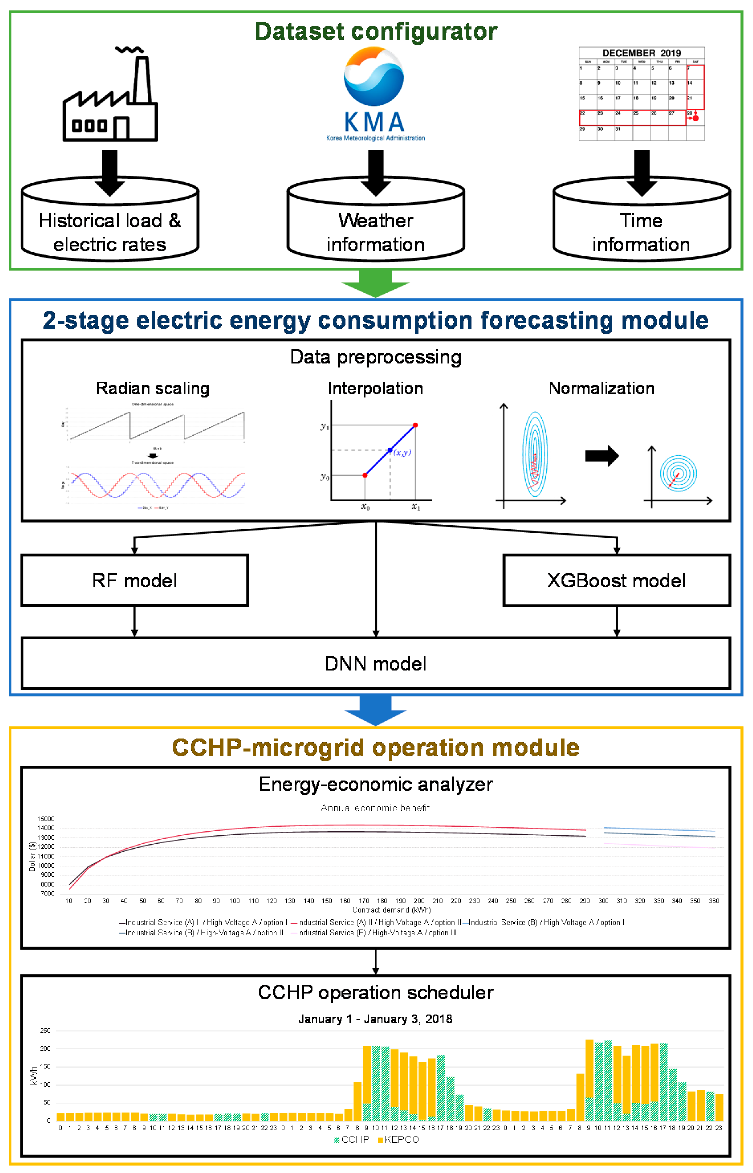
In this paper, we propose a novel two-stage STLF scheme based on nonlinear combination of forecasting methods to solve this problem. In the first stage, we build two STLF models based on extreme gradient boosting (XGBoost) and random forest (RF), which are known to be popular tree-based ensemble models in time series prediction. In the second stage, we build a deep neural network (DNN)-based STLF model to combine the predicted values of XGBoost and RF. Further, we propose an economic analysis-based operation scheduling scheme for CCHP to effectively utilize the results of the STLF. For instance, in Korea, electric rates and contract demand, especially for industrial services should be considered in the electric rate system. Contract demand indicates the instantaneous peak load contracted with the power supply company. Based on the contract demands, a power supply company can make a stable power plan. Basically, the lower the contract demand is, the lower the basic electricity bill is. Hence, to derive more accurate contract demands, the following policy is used: If the consumer sets the contract demand too low, a progressive tax penalty will be added to the excess power, which results in higher electricity charges. On the contrary, if the contract demand is set too high, consumers have to pay unnecessarily high electricity bills. The economic analysis shows the electric rate and contract demand that should be made to achieve the lowest electric charges. In order to intuitively display the outcome of the economic analysis, a graphical representation of CCHP scheduling is shown with the amount of economic benefits gained from the schedule. Figure 1 shows the overall architecture of our scheme.
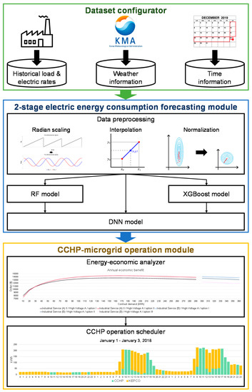
Figure 1.
Overall system architecture.
The main contributions of this paper are as follows:
- (1)
- We propose a novel two-stage STLF scheme that can predict electric energy consumption accurately compared to other previous methods.
- (2)
- We propose a method to generate an optimal operation schedule of CCHP based on the predictive values of electric energy consumption and electric/gas charges in South Korea.
- (3)
- We propose a method to minimize the electric charge by calculating optimal contract demand and electric rate.
The rest of this paper is organized as follows: In Section 2, related studies on STLF are reviewed. In Section 3, we explain the input variables for constructing the STLF model. In Section 4, we describe the structure of our forecasting model, and then, explain how to make CCHP operational scheduling in Section 5. In Section 6, we describe some of the experiments for performance evaluation of the proposed model and CCHP operation scheduling. Finally, in Section 7 we summarize our study.
2. Related Works
So far, many studies have been done to efficiently perform STLF. In recent years, diverse machine learning algorithms in particular have been tested to build more accurate STLF models [21]. In this section, we first introduce diverse STLF models and then describe our previous works for STLF.
2.1. Short-Term Load Forecasting
Typical approaches for STLF have been applied to statistical and machine learning methods for diverse external information such as time factors, weather conditions, and so on. Table 1 summarizes STLF-related studies using statistical techniques and machine learning. Veghefi et al. [22] proposed an STLF model based on the Cochrane–Orcutt estimation technique that combines the multiple linear regression (MLR) and seasonal auto-regressive integrated moving average (SARIMA) models to predict cooling and electric energy consumption effectively. Bagnasco et al. [23] constructed an artificial neural network (ANN)-based STLF model considering holiday indicators and weather conditions as input variables for forecasting electric energy consumption of Cellini Medical Clinic. Powell et al. [24] constructed an STLF model based on a nonlinear autoregressive model with exogenous inputs (NARX) for heating, cooling, and electric energy consumption of a district energy system. This study was unique because it covered a large-scale district energy system that simultaneously produced combined heat and power (CHP), chilled water thermal energy storage (TES), gas turbines, steam turbines, heat recovery steam generators (HRSGs), and auxiliary boilers for a large campus. Jurado et al. [25] constructed several prediction models using RF, ANN, and fuzzy inductive reasoning (FIR). They then compared the prediction models with an ARIMA model by predicting electric energy consumptions in three different buildings at Catalonia Technical University, Catalonia, Spain. They confirmed that FIR showed the best prediction performance. Sandels et al. [26] presented a data analysis framework for identifying and generating models that can predict energy consumption on load level in North European office building floors. The models were based on a simplified statistical approach that did not require detailed knowledge about the office building floor. Grolinger et al. [27] constructed two STLF models based on support vector regression (SVR) and ANN. They considered time data, historical electric load data, and event information and compared their prediction performances with other methods for a large entertainment building in Canada. With daily data, the ANN model achieved better accuracy than the SVR. Gerossier et al. [28] presented a forecasting model for hourly household electric load based on quantile smoothing spline regression using the previous day’s hourly load, last week’s mid-load, and temperature. They computed the mean of the predicted quantile distribution and used it as a single-point forecast. These statistical approaches exhibited excellent performance for simple demand patterns but inaccurate prediction performance for intricate demand patterns. Chen et al. [29] developed a combination of a hybrid SVR model and multiresolution wavelet decomposition (MWD) to predict the hourly electric energy consumption of a hotel and mall. Dong et al. [30] proposed a seasonal SVR with a chaotic cuckoo search (CCS) named SSVRCCS to predict electric energy consumptions in the National Electricity Market and New York Independent System Operator. By using the CCS model, their proposed model can enlarge the population in cuckoo search (CS) to prevent the local optimal problem and increased the search space. By using the seasonal SVR model, it can deal with the seasonal cyclic nature of electric load for accurate and better prediction. However, the computational time is increased due to a large number of iterations. Fan et al. [31] proposed a novel electricity load forecasting model by hybridizing the phase space reconstruction (PSR) algorithm with the bi-square kernel (BSK) regression model, namely the PSR-BSK model. The authors investigated the performance of the model using an hourly dataset of NYISO, USA, and New South Wales market. Hong et al. [32] proposed an electric load prediction model, namely the H-EMD-SVR-PSO model, which combines the empirical mode decomposition (EMD) method, particle swarm optimization (PSO) algorithm, and SVR, to improve predictive accuracy. Based on electrical load data from the Australian electricity market, experimental results showed that the proposed H-EMD-SVR-PSO model received more satisfactory prediction performance than other comparable models.

Table 1.
Summary of several approaches for short-term load forecasting.
These studies suggested the construction of non-generic forecasting models by considering the characteristics of buildings and microgrids. On the other hand, CCHP can be installed and used in various places with possibly different features. Moreover, different types of schedules may be required for CCHP depending on electric energy consumption patterns.
2.2. Our Previous Works
In this section, we briefly describe several STLF models that we proposed in our previous studies and their differences from the proposed model.
In [33], we built two STLF models using the ANN and SVR for four building clusters of a private university in South Korea. For the prediction, we considered not only weather information and time data but also university events, office hours, and class hours. Subsequently, we evaluated the prediction performance of each model by using 5-fold cross-validation. The comparison showed that the ANN-based forecasting model had better performance than the SVR-based model. In [34], we proposed another STLF model based on an auto-encoder (AE) and RF. The AE was used to extract weather information features and time factors effectively. We constructed an RF-based forecasting model using feature extraction values and historical electric loads for day-ahead electric load forecasting. The model was evaluated using the electric energy consumption data of university campuses and the results showed that it gave a better performance than the proposed model in [33]. In [35], we proposed a recurrent inception convolution neural network (RICNN) that combines recurrent neural networks (RNN) and 1-dimensional convolutional neural networks (CNN) to forecast multiple short-term electric loads (48 time steps with an interval of 30 min). A 1-D convolution inception module was used to calibrate the prediction time and hidden state vector values calculated from nearby time steps. By doing so, the inception module could generate an optimized network via the prediction time generated in the RNN and nearby hidden state vectors. The proposed RICNN model was verified using the electric energy consumption data of three large distribution complexes in South Korea. In [36], we constructed diverse ANN models using different numbers of hidden layers and diverse activation functions and compared their performances in a 30 min STLF resolution. To compare the prediction performance, we considered electric load data collected for two years from five different types of buildings (including the dataset used in this study). The comparison showed that a scaled exponential linear unit (SELU)-based ANN model with five hidden layers had a better average performance than other ANN-based STLF models. In [37], we proposed a two-stage electric load forecasting model that combined XGBoost and RF using MLR for the efficient operation of CCHP. To construct this model, an hourly load forecasting was performed using XGBoost and RF. The forecasting results were then combined using a sliding-window based MLR to reflect the energy consumption pattern. The model had a better prediction performance compared with several popular single algorithm-based forecasting models.
The difference between the papers mentioned above and our paper is as follows.
The models in [33] were tailored for university campuses; they were challenging to apply for other types of buildings. The model in [34] used AE to extract features. However, since the performance of AE heavily depends on the size of the training set, it is challenging to show excellent performance if there is not enough quantity of data. In [35], we proposed the RICNN model. However, the RICNN, which purposed a probabilistic approach, is a different purpose because we focus on day-ahead point load forecasting. In [36], the SELU-based ANN model with five hidden layers showed that the dataset we used in this study exhibited insufficient prediction accuracy compared to the other building types because its electric loads are close to zero. In [37], we proposed a two-stage electric load forecasting model to combine XGBoost and RF using MLR. However, to use the forecasted values from one-stage more efficiently, we have to consider existing input variables. Eventually, we further develop our research and propose integrated applications with CCHP operation scheduling and electric rate recommendations, not just ending with forecasts.
3. Input Variable Configuration
In this study, we use hourly electric energy consumption data collected from 1 January 2015 to 31 December 2018 from an industrial building in Incheon, South Korea. Table 2 summarizes some statistics of the collected data. To construct our STLF model, we consider time factors, weather information, historical electric energy consumption, and electric rates for input variable configuration. The details are described in the following subsections.

Table 2.
Statistics of energy consumption data from industrial building.
3.1. Time Data
As time is a very critical factor in the trends of electric energy consumption, we consider all variables that express time such as month, day, hour, day of the week, and holiday. Table 3 shows a list of the time factors we considered as input variables. Herein, month, day, and hour have a sequence form. It is difficult to reflect periodic information in machine learning algorithms when data are in a sequential format. Therefore, we enhanced the data to 2-dimensional data through the periodic function [36]. Table 4 summarizes some regression statistics of 1-dimensional, 2-dimensional, and 1-dimensional + 2-dimensional time factors. The table shows that 1-dimensional + 2-dimensional space data can represent the time factor most effectively. Therefore, we use both 1-dimensional data and continuous 2-dimensional data to represent time factor.

Table 3.
Input variables of time factors.

Table 4.
Regression statistics of time data representation.
3.2. Weather Data
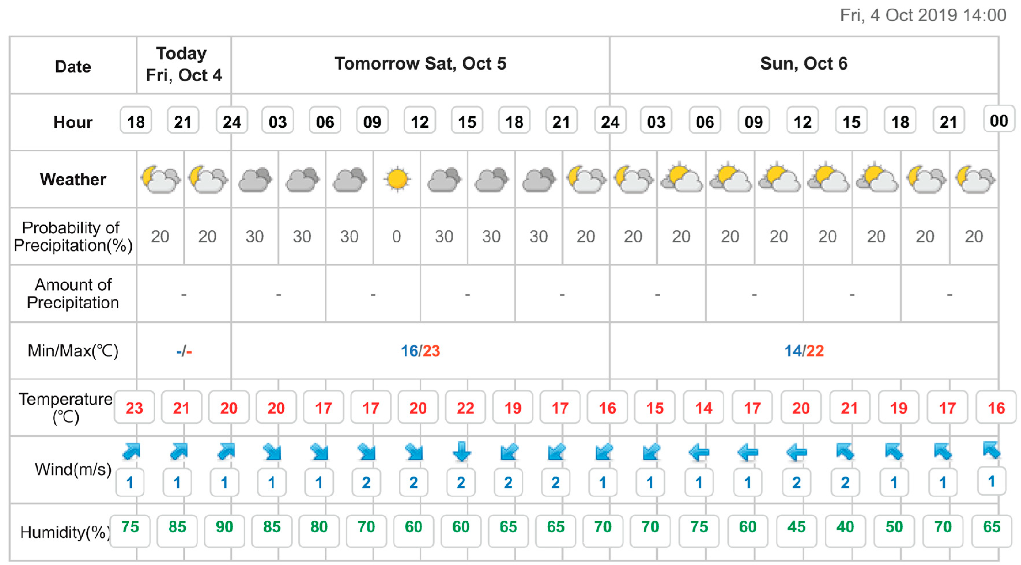
Because the frequency of use of high-power consumption products such as air conditioners and radiators is closely related to weather [38], weather conditions have generally been used for constructing STLF models in many studies [39]. In South Korea, various weather forecast information including temperature, humidity, wind speed, and so on are provided by the Korea Meteorological Administration (KMA). However, KMA provides weather data using two different time resolutions depending on the type of forecast. Very short-term weather forecast provides weather data up to 4 h by 30 min resolution, and short-term weather forecast provides weather data resolution up to 67 h by 3 h resolution. Since our goal is to predict day-ahead electric energy consumption, we need weather data for up to 24 h. Thus, we used the short-term weather forecast data that have 3 h resolution and used linear interpolation to calculate 1 h weather forecast data from them. The short-term weather forecast data consists of values such as daily minimum temperature, daily average temperature, daily maximum temperature, temperature, humidity, wind speed, and precipitation, as shown in Figure 2.
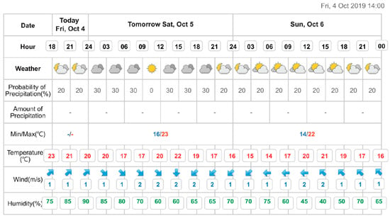
Figure 2.
Example of short-term weather forecast information provided by KMA.
In addition, to establish a more direct correlation between weather data and electric energy consumption, we considered the discomfort index (DI) [40] and wind chill (WC) [41]. DI and WC are defined using Equations (1) and (2), respectively. Here, T, H, and WS represent the temperature, humidity, and wind speed, respectively.
As a result, we use nine types of weather data (i.e., daily maximum temperature, daily average temperature, daily minimum temperature, temperature, humidity, wind speed, precipitation, discomfort index, and wind chill) for the STLF model construction. Table 5 summarizes an example of weather conditions considered for the input variables.

Table 5.
An example of weather conditions on December 25, 2018.
3.3. Historical Electric Energy Consumption
Historical electric energy consumption is a good indicator of electric usage forecasts as it shows electricity usage patterns and trends [42]. We consider a specific time for 10 different days to reflect historical electric energy consumption. Herein, the historical electric energy consumption we considered included the last six days and the same day of the previous four weeks. For instance, if the forecast time is Saturday, 29 June 2019, 4 p.m., we use historical load data measured at 4 p.m. from 1, 8, 15, 22, 23, 24, 25, 26, 27, and 28 June. However, the weekday and weekend load patterns could be different. To reflect trends through historical load data more accurately, we use additional data that indicate whether the ten days used as input variables were holidays or not.
3.4. Electric Rates
Because one of the operational goals of the smart grid is to reduce electric charges, many STLF studies have used electric rate information as one of the input variables [43]. Thus, we also consider information on electric rates as input variables [44]. In South Korea, three different sections are used by Korea Electric Power Corporation (KEPCO) for electric rate: off-peak, mid-peak, and on-peak loads [45]. Electric rates are determined by the amount of electric energy consumption, the intended use of the building (i.e., residential, general, educational, industrial, etc.) and the season or month. As in the day of the week and holiday data, one-hot encoding method is used to represent the electric rate information. Hence, depending on the time and rate section, the input variable is set to 1; otherwise, it is set to zero.
4. Two-Stage STLF Model Construction
So far, various single algorithm-based STLF models have been proposed [46]. Even though they showed good performance in the domains that were focused on, their performance was limited in the other domains or electric energy consumption patterns were intricate. To alleviate this limitation, we propose a two-stage day-ahead STLF model that combines two single algorithm-based STLF models using DNNs.
4.1. The First Stage: Constructing Two STLF Models
In the first stage, we build two STLF models based on XGBoost and RF, which are well-known tree-based ensemble models in time series prediction [47], by using various input variables. They are based on boosting and bootstrap aggregating (bagging) algorithms, respectively. Compared to other boosting algorithms and bagging algorithms, the XGBoost and RF models show better predictive accuracy and have the highest correlation with actual power consumption. In addition, as XGBoost supports various loss functions, we can choose an appropriate loss function depending on the characteristics of the data. On the contrary, it suffers from overfitting during training [48]. RF can handle high dimensional data well, but it cannot give precise value for the regression model because the final prediction is the average of all the predictions from the subset trees [49]. By using the predicted values of the XGBoost model and the RF model together with other input variables, it is possible to prevent overfitting and to make more accurate prediction.
4.1.1. Extreme Boosting Machine
XGBoost, which was proposed by Chen and Guestrin [50], is a scalable machine learning model used in tree-boosting. It has been widely used for forecasting purposes such as STLF and store sales forecasting [51]. The basic principle of XGBoost is boosting, which combines a weak basic learning model with an active learner in an iterative fashion [52]. At each iteration of boosting, the residuals can modify the previous predictor to optimize the specified loss function. XGBoost provides faster learning and expandability based on parallel and distributed computing by further developing the existing boosting technique. It establishes an objective function to measure model performance by adding regularization to loss functions to improve performance. In addition, missing values can be handled easily because they are recognized and automatically supplemented to perform boosting. XGBoost gradually increases the depth of the tree at the beginning of learning. If the gain information obtained in the tree with increased depth is smaller than the of Gamma value, the depth stops increasing.
4.1.2. Random Forest
RF is a flexible machine learning algorithm that produces excellent results even without hyper parameter tuning. It has become one of the most commonly used machine learning algorithms because it can be easily used for classification and regression. Moreover, it can work efficiently on a large amount of data and handle thousands of input variables without deleting them, which is why it performs well. The basic principle of RF is called the bagging algorithm [53]. Bagging is an ensemble algorithm designed to improve the stability and accuracy of individual forecasting models such as decision trees. It selects a random sample of size n from the training set, fits it in the individual forecasting models, and produces a result that is averaged or voted on all individual forecasting models. The bagging algorithm in RF helps reduce the variance and influence of overfitting of decision trees.
4.2. The Second Stage: Combining STLF Models Using DNN
An ANN, which is also known as a multilayer perceptron (MLP), is a type of machine learning algorithm that is a feed-forward neural network architecture with an input layer, hidden layer, and output layer [54]. It aims to learn the nonlinear and complex structure of data by duplicating human brain functions [55]. Each layer in the neural network consists of several nodes. Each node receives values from the nodes in the previous layer to determine the output and provide values for the nodes in the next layer. As this process repeats, the nodes in the output layer provide the required values [56]. The number of hidden layers determines whether the network is deep or shallow. For instance, when the number of hidden layers is two or more, then the network is called a deep neural network [57]. Recently, various DNN models have shown excellent prediction performances due to the remarkably improved computing performance [58].
In the second stage, we construct an STLF model by combining the results of the two STLF models built in the first stage using a DNN. For training the DNN model, we used the predicted values of XGBoost and RF as input variables to reflect the characteristics of bagging and boosting algorithms. We also considered time factors, weather data, historical electric energy consumption data, and electric rate as input variables to further improve the forecasting performance. In our DNN model, we use the SELU function as an activation function and the number of hidden layers is set as five [36]. Additionally, the number of neurons in the hidden layer is set by two thirds of the number of input variables [59].
5. Economic Analysis Based CCHP Operation Scheduling
CCHP is known to improve energy utilization, reduce energy costs, and respond to peak loads by using thermal energy generated from the power generation process for heating and cooling. In addition, by using natural gas, CCHP can be a solution to environmental pollution [60]. Natural gas is a relatively clean-burning fossil fuel [61]. Burning natural gas for energy gives fewer emissions of nearly all types of air pollutants and carbon dioxide than burning coal or petroleum products to produce an equal amount of energy [62]. In this section, to see the applicability of our proposed scheme, we describe how daily CCHP operation scheduling can be made based on the forecasted daily electric energy consumption of 1 h resolution. In particular, we consider natural gas as the primary energy source of CCHP, and the economic benefit of CCHP operation is changed according to power generation efficiency. Hence, for its economic analysis, the cost of natural gas consumed in power generation must be determined by the power generation efficiency. Table 6 summarizes the gas charge sections of the industrial service in South Korea.

Table 6.
Gas charge sections for industrial buildings.
The electric rate system should be considered for a more accurate economic analysis. There are several considerations in the electric rate system of South Korea.
- The electric rate system divides the types of contracts according to the purpose of electricity usage, and applies the corresponding charges. The contract types are divided into six classes, namely, residential, general, industrial, educational, agricultural, and streetlights service. Some contract types have more granular rates, depending on the size of the voltage or the contract demand.
- The electric rate consists of the demand and energy charges. The demand charge recovers the fixed costs related to the electric energy supply equipment. It is determined based on the contract demand or peak load. On the other hand, the energy charge recovers the variable costs in proportion to usage.
- Seasonal and hourly differential electric rates are applied to some contract types, including industrial and general service. To reflect the differences in supply costs by time zone according to seasonal demand, high rates are charged in seasons and time zones with high electric energy consumption, and low rates are applied in seasons and time zones with low electric energy consumption.
- The electric rate system offers three options depending on the relative amount of the demand and energy charges: Option I, Option II, and Option III. For the demand charge, Option I > Option II > Option III and for the energy charges, Option I < Option II < Option III. These options are for reducing energy consumption, inducing voluntary peak time load management, and ultimately reducing the cost of power equipment by enabling consumers to select an electric rate depending on their load pattern.
As we focus on the industrial building in this study, we have more refined electric rates depending on the supply voltage and the contract demand. First, depending on whether the contract demand exceeds 300 kW or not, there are two electric rates: Type A and Type B. For each rate, there are four groups depending on the size of the supply voltage: low voltage, high voltage A, high voltage B, and high voltage C. Each group then offers three options: Option I, Option II, and Option III. Table 7 summarizes the electric rates for Industrial Service (B), High Voltage A, and Option I. Industrial service (B) is an electric rate that can be used when contract demand is more than 300 kW.

Table 7.
An example of electric rates table for an industrial building.
Operation scheduling is created to maximize annual economic benefits. Equations (3)–(6) represent detailed formulas for calculating annual economic benefits. Economic benefits are composed of two parts: (i) reduced electric charges, which are the direct economic benefits of using CCHP, and (ii) reduced heating/cooling charges by using thermal energy generated by CCHP. In the experiment, we assume CCHP can make 1.43 Mcal of thermal energy while generating 1 kWh [63]. We calculate how much it would cost to obtain this 1.43 Mcal of thermal energy using electric energy and reflect it in the formulas. Algorithm 1 shows the generation of an operational schedule for maximizing annual economic benefits. Basically, the schedule tells how much energy should be generated by CCHP and how much energy should be supplied by the public power system for each scheduling hour.
| Algorithm 1. CCHP operation scheduling |
| Input: month m, day d, hour h Output: generation amount of CCHP , supply amount of public system if else if = = 0 else if = = else = 0 = return , |
6. Experimental Results
6.1. Comparison of Prediction Performance with Various STLF Models
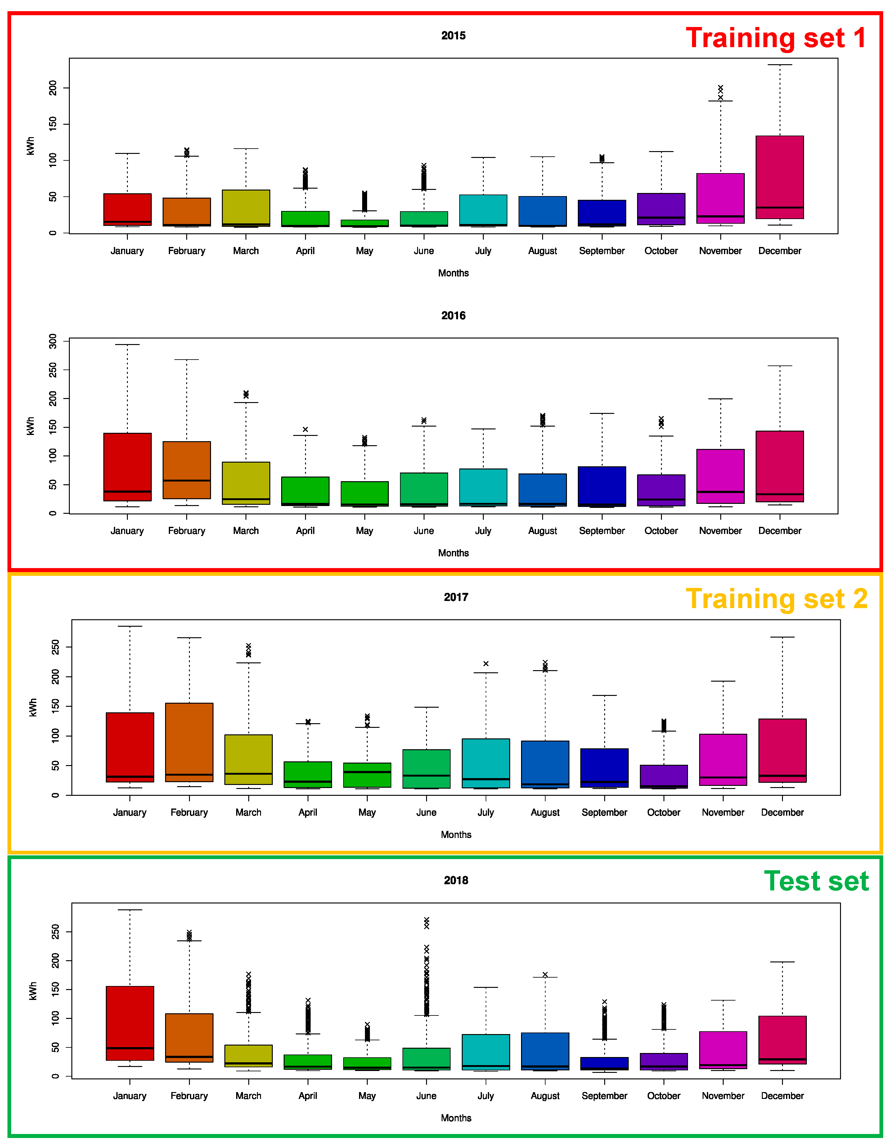
In this paper, we compare popular machine learning algorithms such as decision tree (DT), gradient boosting machine (GBM), bagging algorithm, and so on, to explain why we chose XGBoost and RF models in the first stage. Besides, we compare the performance with the prediction model (Persistence) which is actually using in the data collection environment. Persistence model uses the previous day (or the corresponding day in the previous week) as a prediction. Persistence implies that future values of the time series are calculated on the assumption that conditions remain unchanged between the current time and future time. As the second stage of our proposed model uses the predicted values of these two models, we divide the dataset into training set 1 (training the first-stage model), training set 2 (training the second-stage model), and test set (forecasting electric energy consumption and economic analysis), at a ratio of 50:25:25. Specifically, data collected from January 2015 to December 2016 was used as training set 1, data collected from January 2017 to December 2017 was used as training set 2, and data collected from January 2018 to December 2018 was used as test set. The performance of each machine learning algorithm was measured using the training set 2. Figure 3 shows monthly energy consumption and divided dataset. In addition, we compare our proposed model with various STLF models composed of different machine learning algorithms in the first-stage, and several forecasting models from our previous studies in the second-stage. To do this, we divided the dataset into training and test sets, at a ratio of 75:25.
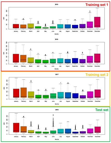
Figure 3.
Box plots by the monthly electric load for separation of training and test sets.
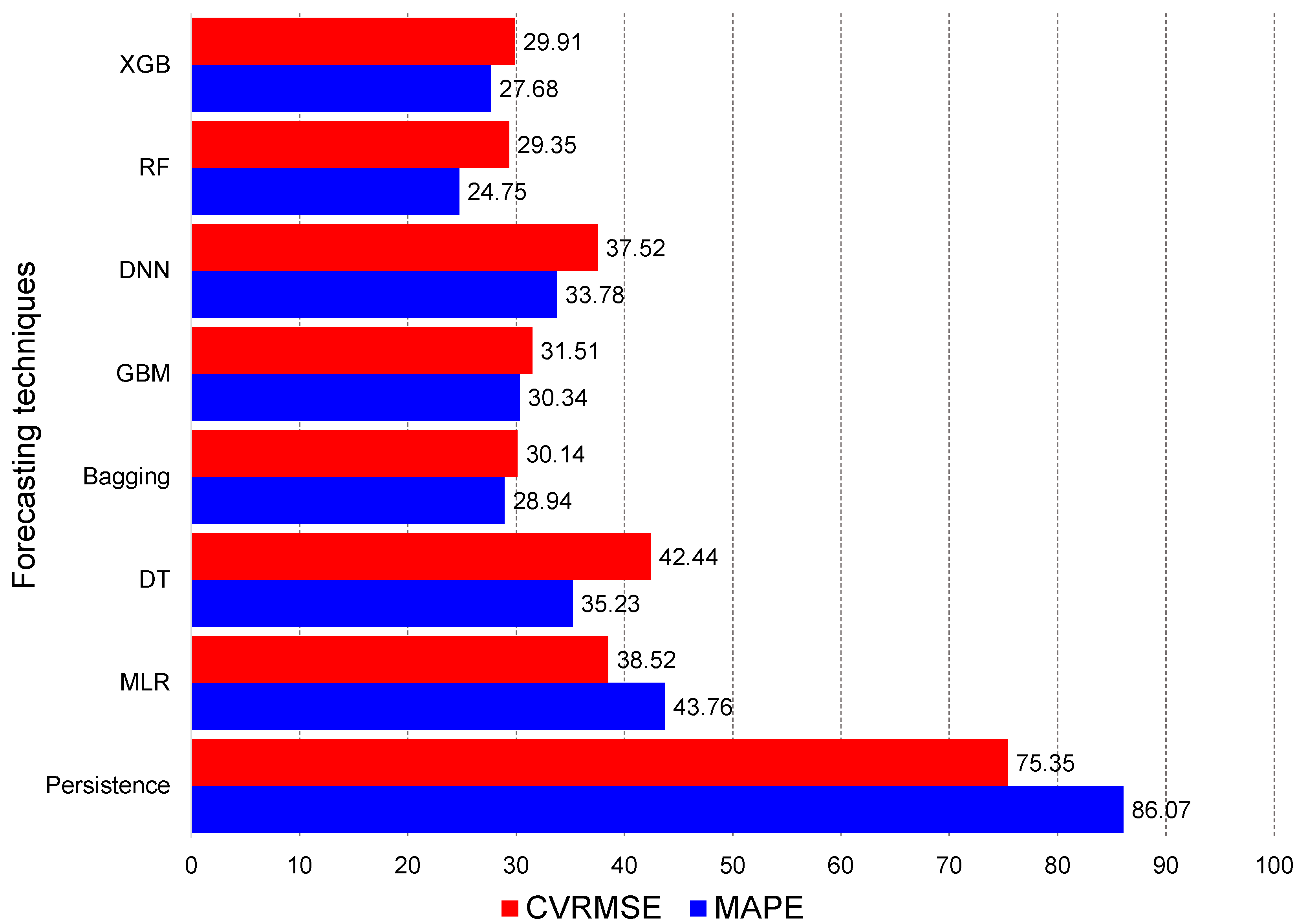
Additionally, we selected a coefficient of variation of the root mean square error (CVRMSE) and mean absolute percentage error (MAPE) because they are easier to understand than other performance indicators such as the root mean square error (RMSE) or mean squared error (MSE) [64]. They were then used to evaluate the prediction performance of the proposed model. The CVRMSE and MAPE equations are shown in (7) and (8), respectively. Here, is the number of time observed, is an average of the actual values. and are the actual and predicted values, respectively. Figure 4 exhibits the comparison of CVRMSE and MAPE results for each machine learning algorithm.

Figure 4.
CVRMSE and MAPE comparison of machine learning algorithms.
As shown in Figure 4, XGBoost and RF models show better prediction performance in training set 2 compared with other machine learning algorithms. The performance of machine learning techniques is better than the persistence model which is a statistical model. In addition, the performance of the XGBoost and RF models was better than the other machine learning algorithms. XGBoost performed well because it allows users to choose an appropriate loss function depending on the characteristics of the data. RF performed well because it can handle high-dimensional data well. Table 8 summarizes the Pearson correlation coefficients between the forecasted values of machine learning algorithms and actual electric energy consumptions. We found that the forecasted values of XGBoost and RF present higher correlation coefficients than those of other machine learning algorithms. Therefore, we used the forecasted values of XGBoost and RF as new input variables for the second stage.

Table 8.
Comparison of the Pearson correlation coefficients.
Table 9, Table 10 and Table 11 summarize the comparison of our proposed model with other 2-stage models and several forecasting models of our previous studies in terms of CVRMSE and MAPE. As summarized in Table 9, Table 10 and Table 11, our proposed model showed an almost better prediction performance than other forecasting models.

Table 9.
MAPE comparison for each month (The best in bold).

Table 10.
CVRMSE comparison for each month (The best in bold).

Table 11.
Statistical analysis of APEs by each forecasting model.
Finally, to ensure the significant contribution in terms of forecasting accuracy improvement for the proposed model, the Wilcoxon test and the Friedman test are conducted [30]. Wilcoxon test was used to test the null hypothesis by setting the null hypothesis to determine whether there was a significant difference between the two models. If the p-value is less than the significance level, the null hypothesis is rejected and the two models are judged to have significant differences. Friedman test is a multiple comparisons test that aims to detect significant differences between the results of two or more algorithms model. The results of the Wilcoxon test with the significance level set to 0.05 are shown in Table 12. Since the p-value in all cases is below the significance level, it was proven that proposed model is superior to the other models.

Table 12.
Results of Wilcoxon test and Friedman test.
6.2. Economic Analysis Based CCHP Operation Scheduling
In this section, we describe how CCHP operation scheduling is made based on economic analysis. To maximize the annual economic benefits, it is also essential to determine the electric rate and amount of contract demand at the same time. We perform an experiment to find the optimal electric rate and contract demand to maximize on economic benefits.
A monthly economic analysis using the test set confirms that the economic benefits are similar to the monthly energy consumption, as shown in Figure 5. We can see that high economic benefits can be obtained in summer and winter when energy consumption is high.
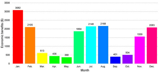
Figure 5.
Monthly economic benefits.
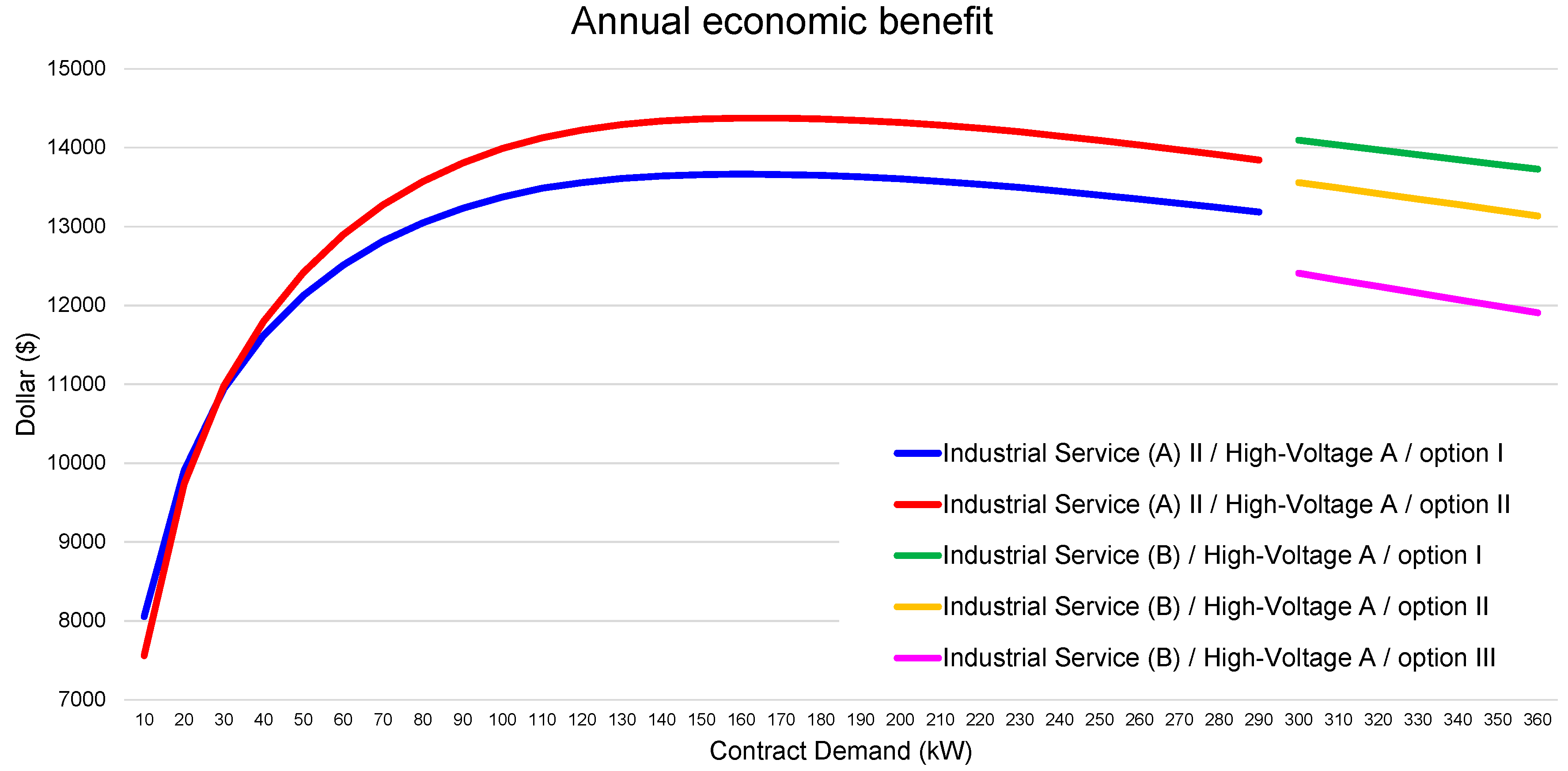
Because the industrial building where the electric energy consumption data was collected is equipped with advanced meters, the electric rate of industrial service (A) II and industrial service (B) can be chosen. In addition, since the building’s supply voltage is between 3300 V and 66,000 V, we choose the high voltage A as the electric rate of the building. Industrial service (A) II has two options, and industrial service (B) has three options. As a result, five different electric rates are compared in the experiment. Figure 6 shows the annual economic benefit of each electric rate based on contract demand.
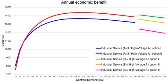
Figure 6.
Annual economic benefit of each electric rate based on contract demand.
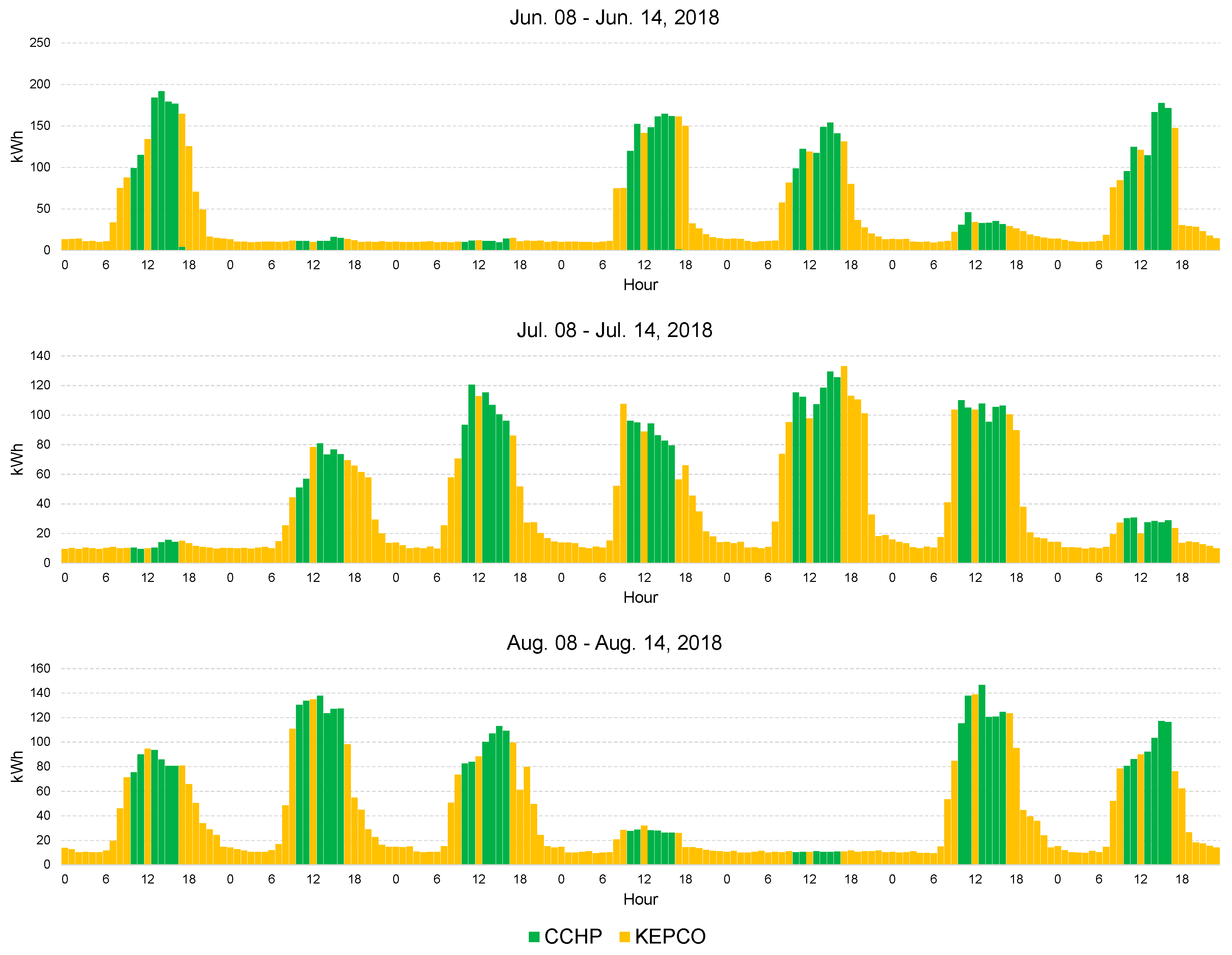
Figure 6 shows that “industrial service (A) II / high voltage A / Option II” electric rate with 160 kW contract demand can make the highest annual economic benefit and Figure 7, Figure 8 and Figure 9 show the scheduling result of the CCHP operation according to this electric rate. In the figure, the yellow boxes represent electric energy supplied by the public power system and the green boxes represent electric energy generated by the CCHP system.
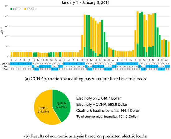
Figure 7.
Example of CCHP operation scheduling.
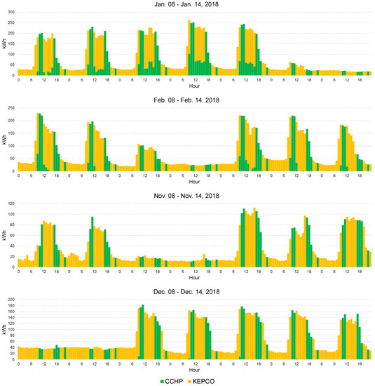
Figure 8.
Example of CCHP operation scheduling in winter.
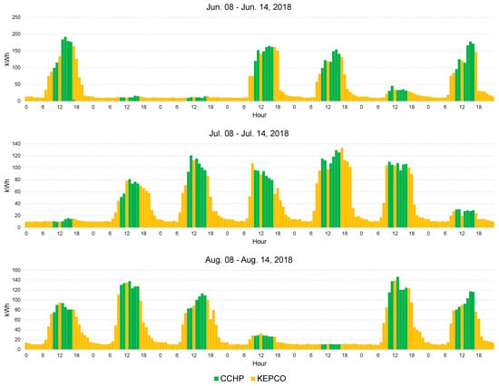
Figure 9.
Example of CCHP operation scheduling in summer.
According to the schedule, an economic benefit of USD 195 can be made when using CCHP with a public power system for three days. Moreover, economic benefits of more than USD 14,000 annually can be achieved by using CCHP with the public power system.
7. Conclusions
In this study, we proposed a novel 2-stage STLF model that combines popular STLF models by using a DNN to further expand the domain of applicability. In the first stage, we used XGBoost and RF algorithms to predict day-ahead electric energy consumption. In the second stage, we built a load forecasting model based on DNN by using the forecasted results of XGBoost and RF and other external data as new input variables. To verify the forecasting performance of our proposed model, we performed day-ahead forecasting using actual factory electric energy consumption data and compared its accuracy with several machine learning methods and our previous forecasting models. The comparison showed that our proposed model showed the best prediction performance in terms of CVRMSE and MAPE.
Additionally, to show the applicability of our model, we performed CCHP operation scheduling based on forecasting and economic analysis, decided the best electric rate and contract demand, and showed how much could be saved by the decision. According to the experiment, the electric cost was reduced by 37% annually.
Author Contributions
All authors have read and agreed to the published version of the manuscript. Conceptualization, S.P. and J.M.; methodology, S.P. and J.M.; software, S.J.; validation, S.P., J.M. and S.J.; formal analysis, S.R. and E.H.; data curation, S.R.; writing—original draft preparation, S.P. and E.H.; writing—review and editing, E.H. and S.W.B.; visualization, S.J.; supervision, E.H.; project administration, E.H. and S.W.B.; funding acquisition, S.R.
Funding
This research was supported in part by the Korea Electric Power Corporation (grant number: R18XA05) and in part by Energy Cloud R&D Program (grant number: 2019M3F2A1073179) through the National Research Foundation of Korea (NRF) funded by the Ministry of Science and ICT.
Conflicts of Interest
The authors declare no conflict of interest.
References
- Tabrizchi, H.; Javidi, M.M.; Amirzadeh, V. Estimates of residential building energy consumption using a multi-verse optimizer-based support vector machine with k-fold cross-validation. Evol. Syst. 2019, 1–13. [Google Scholar] [CrossRef]
- Morandin, M.; Bolognani, S.; Faggion, A. Active Torque Damping for an ICE-Based Domestic CHP System with an SPM Machine Drive. IEEE Trans. Ind. Appl. 2015, 51, 3137–3146. [Google Scholar] [CrossRef]
- Lee, S.K.; Mogi, G. Relative efficiency of energy technologies in the Korean mid-term strategic energy technology development plan. Renew. Sustain. Energy Rev. 2018, 91, 472–482. [Google Scholar] [CrossRef]
- Kenner, S.; Thaler, R.; Kucera, M.; Volbert, K.; Waas, T. Smart Grid Architecture for Monitoring and Analyzing, Including Modbus and REST Performance Comparison. In Proceedings of the 2015 12th International Workshop on Intelligent Solutions in Embedded Systems (WISES), Ancona, Italy, 29–30 October 2015; pp. 91–96. [Google Scholar]
- Saponara, S.; Saletti, R.; Mihet-Popa, L. Hybrid Micro-Grids Exploiting Renewables Sources, Battery Energy Storages, and Bi-Directional Converters. Appl. Sci. 2019, 9, 4973. [Google Scholar] [CrossRef]
- Ding, Z.; Lee, W.J.; Wang, J. Stochastic Resource Planning Strategy to Improve the Efficiency of Microgrid Operation. In Proceedings of the 2014 IEEE Industry Application Society Annual Meeting, Vancouver, BC, Canada, 5–9 October 2014; IEEE: Piscataway, NJ, USA, 2014. [Google Scholar]
- Banerji, A.; Biswas, S.K.; Singh, B. Enhancing Quality of Power to Sensitive Loads with Microgrid. IEEE Trans. Ind. Appl. 2015, 52, 360–368. [Google Scholar] [CrossRef]
- Pantaleo, A.M.; Camporeale, S.; Shah, N. Natural gas-biomass dual fuelled microturbines: Comparison of operating strategies in the Italian residential sector. Appl. Therm. Eng. 2014, 71, 686–696. [Google Scholar] [CrossRef]
- Mortaji, M.; Ow, S.H.; Moghavvemi, M.; Almurib, H.A.F. Load Shedding and Smart-Direct Load Control Using Internet of Things in Smart Grid Demand Response Management. IEEE Trans. Ind. Appl. 2017, 53, 5155–5163. [Google Scholar] [CrossRef]
- Zhu, R.; Guo, W.; Gong, X. Short-Term Load Forecasting for CCHP Systems Considering the Correlation between Heating, Gas and Electrical Loads Based on Deep Learning. Energies 2019, 12, 3308. [Google Scholar] [CrossRef]
- Sun, Z.; Li, L.; Bego, A.; Dababneh, F. Customer-side electricity load management for sustainable manufacturing systems utilizing combined heat and power generation system. Int. J. Prod. Econ. 2015, 165, 112–119. [Google Scholar] [CrossRef]
- Chen, Y.T. The Factors Affecting Electricity Consumption and the Consumption Characteristics in the Residential Sector—A Case Example of Taiwan. Sustainability 2017, 9, 1484. [Google Scholar] [CrossRef]
- Mocanu, E.; Nguyen, P.H.; Gibescu, M.; Kling, W.L. Deep Learning for Estimating Building Energy Consumption. Sustain. Energy Grids Netw. 2016, 6, 91–99. [Google Scholar] [CrossRef]
- Ahmad, A.S.; Hassan, M.Y.; Abdullah, M.P.; Rahman, H.A.; Hussin, F.; Abdullah, H.; Saidur, R. A review on applications of ANN and SVM for building electrical energy consumption forecasting. Renew. Sustain. Energy Rev. 2014, 33, 102–109. [Google Scholar] [CrossRef]
- Hong, T.; Fan, S. Probabilistic electric load forecasting: A tutorial review. Int. J. Forecast. 2016, 32, 914–938. [Google Scholar] [CrossRef]
- Dedinec, A.; Filiposka, S.; Dedinec, A.; Kocarev, L. Deep Belief Network based Electricity Load Forecasting: An Analysis of Macedonian Case. Energy 2016, 115, 1688–1700. [Google Scholar] [CrossRef]
- Guo, Y.; Nazarian, E.; Ko, J.; Rajurkar, K. Hourly cooling load forecasting using time-indexed ARX models with two-stage weighted least squares regression. Energy Convers. Manag. 2014, 80, 46–53. [Google Scholar] [CrossRef]
- Fan, S.; Chen, L. Short-term load forecasting based on an adaptive hybrid method. IEEE Trans. Power Syst. 2006, 21, 392–401. [Google Scholar] [CrossRef]
- Tian, C.; Hao, Y. A novel nonlinear combined forecasting system for short-term load forecasting. Energies 2018, 11, 712. [Google Scholar] [CrossRef]
- Kim, J.C.; Cho, S.M.; Shin, H.S. Advanced power distribution system configuration for smart grid. IEEE Trans. Smart Grid 2013, 4, 353–358. [Google Scholar] [CrossRef]
- Armstrong, J.S. Combining Forecasts: The End of the Beginning or the Beginning of the End? Int. J. Forecast. 1989, 5, 585–588. [Google Scholar] [CrossRef]
- Vaghefi, A.; Jafari, M.A.; Bisse, E.; Lu, Y.; Brouwer, J. Modeling and forecasting of cooling and electricity load demand. Appl. Energy 2014, 136, 186–196. [Google Scholar] [CrossRef]
- Bagnasco, A.; Fresi, F.; Saviozzi, M.; Silvestro, F.; Vinci, A. Electrical consumption forecasting in hospital facilities: An application case. Energy Build. 2015, 103, 261–270. [Google Scholar] [CrossRef]
- Powell, K.M.; Sriprasad, A.; Cole, W.J.; Edgar, T.F. Heating, cooling, and electrical load forecasting for a large-scale district energy system. Energy 2014, 74, 877–885. [Google Scholar] [CrossRef]
- Jurado, S.; Nebot, À.; Mugica, F.; Avellana, N. Hybrid methodologies for electricity load forecasting: Entropy-based feature selection with machine learning and soft computing techniques. Energy 2015, 86, 276–291. [Google Scholar] [CrossRef]
- Sandels, C.; Widén, J.; Nordström, L.; Andersson, E. Day-ahead predictions of electricity consumption in a Swedish office building from weather, occupancy, and temporal data. Energy Build. 2015, 108, 279–290. [Google Scholar] [CrossRef]
- Grolinger, K.; L’Heureux, A.; Capretz, M.A.; Seewald, L. Energy forecasting for event venues: Big data and prediction accuracy. Energy Build. 2016, 112, 222–233. [Google Scholar] [CrossRef]
- Gerossier, A.; Girard, R.; Kariniotakis, G.; Michiorri, A. Probabilistic Day-Ahead Forecasting of Household Electricity Demand. CIRED-Open Access Proc. J. 2017, 2017, 2500–2504. [Google Scholar] [CrossRef]
- Chen, Y.; Tan, H. Short-term prediction of electric demand in building sector via hybrid support vector regression. Appl. Energy 2017, 204, 1363–1374. [Google Scholar] [CrossRef]
- Dong, Y.; Zhang, Z.; Hong, W.C. A hybrid seasonal mechanism with a chaotic cuckoo search algorithm with a support vector regression model for electric load forecasting. Energies 2018, 11, 1009. [Google Scholar] [CrossRef]
- Fan, G.F.; Peng, L.L.; Hong, W.C. Short term load forecasting based on phase space reconstruction algorithm and bi-square kernel regression model. Appl. Energy 2018, 224, 13–33. [Google Scholar] [CrossRef]
- Hong, W.C.; Fan, G.F. Hybrid Empirical Mode Decomposition with Support Vector Regression Model for Short Term Load Forecasting. Energies 2019, 12, 1093. [Google Scholar] [CrossRef]
- Moon, J.; Park, J.; Hwang, E.; Jun, S. Forecasting power consumption for higher educational institutions based on machine learning. J. Supercomput. 2018, 74, 3778–3800. [Google Scholar] [CrossRef]
- Son, M.; Moon, J.; Jung, S.; Hwang, E. A Short-Term Load Forecasting Scheme Based on Auto-Encoder and Random Forest. In Proceedings of the 3rd International Conference on Applied Physics, System Science and Computers (APSAC), Dubrovnik, Croatia, 26–28 September 2018; pp. 138–144. [Google Scholar]
- Kim, J.; Moon, J.; Hwang, E.; Kang, P. Recurrent inception convolution neural network for multi short-term load forecasting. Energy Build. 2019, 194, 328–341. [Google Scholar] [CrossRef]
- Moon, J.; Park, S.; Rho, S.; Hwang, E. A comparative analysis of artificial neural network architectures for building energy consumption forecasting. Int. J. Distrib. Sens. Netw. 2019, 15, 1550147719877616. [Google Scholar] [CrossRef]
- Park, S.; Moon, J.; Hwang, E. 2-Stage Electric Load Forecasting Scheme for Day-Ahead CCHP Scheduling. In Proceedings of the 13th IEEE International Conference on Power Electronics and Drive Systems (PEDS), Toulouse, France, 9–12 July 2019. [Google Scholar]
- Moon, J.; Kim, Y.; Son, M.; Hwang, E. Hybrid Short-Term Load Forecasting Scheme Using Random Forest and Multilayer Perceptron. Energies 2018, 11, 3283. [Google Scholar] [CrossRef]
- Wang, P.; Liu, B.; Hong, T. Electric load forecasting with recency effect: A big data approach. Int. J. Forecast. 2016, 32, 585–597. [Google Scholar] [CrossRef]
- Xie, J.; Chen, Y.; Hong, T.; Laing, T.D. Relative humidity for load forecasting models. IEEE Trans. Smart Grid 2016, 9, 191–198. [Google Scholar] [CrossRef]
- Xie, J.; Hong, T. Wind speed for load forecasting models. Sustainability 2017, 9, 795. [Google Scholar] [CrossRef]
- Iglesias, F.; Kastner, W. Analysis of similarity measures in times series clustering for the discovery of building energy patterns. Energies 2013, 6, 579–597. [Google Scholar] [CrossRef]
- Lee, W.; Jung, J.; Lee, M. Development of 24-hour optimal scheduling algorithm for energy storage system using load forecasting and renewable energy forecasting. In Proceedings of the 2017 IEEE Power & Energy Society General Meeting (PESGM), Chicago, IL, USA, 16–20 July 2017. [Google Scholar]
- Raza, M.Q.; Khosravi, A. A review on artificial intelligence based load demand forecasting techniques for smart grid and buildings. Renew. Sustain. Energy Rev. 2015, 50, 1352–1372. [Google Scholar] [CrossRef]
- Lee, W.; Jung, J.; Kang, B.O. Cost-Benefit Analysis for Industrial Customers-Installed Energy Storage System in South Korea. In Proceedings of the 2018 IEEE Innovative Smart Grid Technologies-Asia (ISGT Asia), Singapore, 22–25 May 2018. [Google Scholar]
- Le, T.; Vo, M.T.; Vo, B.; Hwang, E.; Rho, S.; Baik, S.W. Improving electric energy consumption prediction using CNN and Bi-LSTM. Appl. Sci. 2019, 9, 4237. [Google Scholar] [CrossRef]
- Lindner, C.; Bromiley, P.A.; Ionita, M.C.; Cootes, T.F. Robust and accurate shape model matching using random forest regression-voting. IEEE Trans. Pattern Anal. Mach. Intell. 2014, 37, 1862–1874. [Google Scholar] [CrossRef] [PubMed]
- Gómez-Ríos, A.; Luengo, J.; Herrera, F. A study on the noise label influence in boosting algorithms: AdaBoost, GBM and XGBoost. In Proceedings of the 12th International Conference, HAIS 2017, La Rioja, Spain, 21–23 June 2017; Springer: Cham, Switzerland, 2017; pp. 268–280. [Google Scholar]
- Qingqing, K.; Xiangqian, D.; Huili, G. Application of improved random forest pruning algorithm in tobacco origin identification of near infrared spectrum. Laser Optoelectron. Prog. 2018, 55, 446–451. [Google Scholar]
- Chen, T.; Guestrin, C. Xgboost: A scalable tree boosting system. In Proceedings of the 22nd ACM SIGKDD International Conference on Knowledge Discovery and Data Mining, San Francisco, CA, USA, 13–17 August 2016. [Google Scholar]
- Ruiz-Abellón, M.; Gabaldón, A.; Guillamón, A. Load forecasting for a campus university using ensemble methods based on regression trees. Energies 2018, 11, 2038. [Google Scholar] [CrossRef]
- Schapire, R.E. The boosting approach to machine learning: An overview. In Nonlinear Estimation and Classification; Springer: Berlin, Germany, 2003; pp. 149–171. [Google Scholar]
- Breiman, L. Bagging predictors. Mach. Learn. 1996, 24, 123–140. [Google Scholar] [CrossRef]
- Liang, Y.; Niu, D.; Hong, W.C. Short term load forecasting based on feature extraction and improved general regression neural network model. Energy 2019, 166, 653–663. [Google Scholar] [CrossRef]
- Baek, S.J.; Yoon, S.G. Short-Term Load Forecasting for Campus Building with Small-Scale Loads by Types Using Artificial Neural Network. In Proceedings of the 2019 IEEE Power & Energy Society Innovative Smart Grid Technologies Conference (ISGT), Washington, DC, USA, 18–21 February 2019. [Google Scholar]
- Liu, P.; Zheng, P.; Chen, Z. Deep Learning with Stacked Denoising Auto-Encoder for Short-Term Electric Load Forecasting. Energies 2019, 12, 2445. [Google Scholar] [CrossRef]
- Ryu, S.; Noh, J.; Kim, H. Deep neural network based demand side short term load forecasting. Energies 2017, 10, 3. [Google Scholar] [CrossRef]
- Shi, H.; Xu, M.; Li, R. Deep learning for household load forecasting—A novel pooling deep RNN. IEEE Trans. Smart Grid 2017, 9, 5271–5280. [Google Scholar] [CrossRef]
- Heaton, J. Introduction to Neural Networks with Java; Heaton Research, Inc.: Chesterfield, MO, USA, 2008; ISBN 1-60439-008-5. [Google Scholar]
- Li, H.; Fu, L.; Geng, K.; Jiang, Y. Energy utilization evaluation of CCHP systems. Energy Build. 2006, 38, 253–257. [Google Scholar] [CrossRef]
- Allen, D.T.; Torres, V.M.; Thomas, J.; Sullivan, D.W.; Harrison, M.; Hendler, A.; Herndon, S.C.; Kolb, C.E.; Fraser, M.P.; Hill, A.D.; et al. Measurements of methane emissions at natural gas production sites in the United States. Proc. Natl. Acad. Sci. USA 2013, 110, 17768–17773. [Google Scholar] [CrossRef]
- Van Ruijven, B.; Van Vuuren, D.P. Oil and natural gas prices and greenhouse gas emission mitigation. Energy Policy 2009, 37, 4797–4808. [Google Scholar] [CrossRef]
- Yun, R. Economic analysis of CHP system for building by CHP capacity optimizer. Korean J. Air-Cond. Refrig. Eng. 2008, 20, 321–326. [Google Scholar]
- Kuo, P.H.; Huang, C.J. A high precision artificial neural networks model for short-term energy load forecasting. Energies 2018, 11, 213. [Google Scholar] [CrossRef]
© 2020 by the authors. Licensee MDPI, Basel, Switzerland. This article is an open access article distributed under the terms and conditions of the Creative Commons Attribution (CC BY) license (http://creativecommons.org/licenses/by/4.0/).

