How Climate Change Affects the Building Energy Consumptions Due to Cooling, Heating, and Electricity Demands of Italian Residential Sector


Abstract
1. Introduction
2. Materials and Methods
3. Results and Discussion
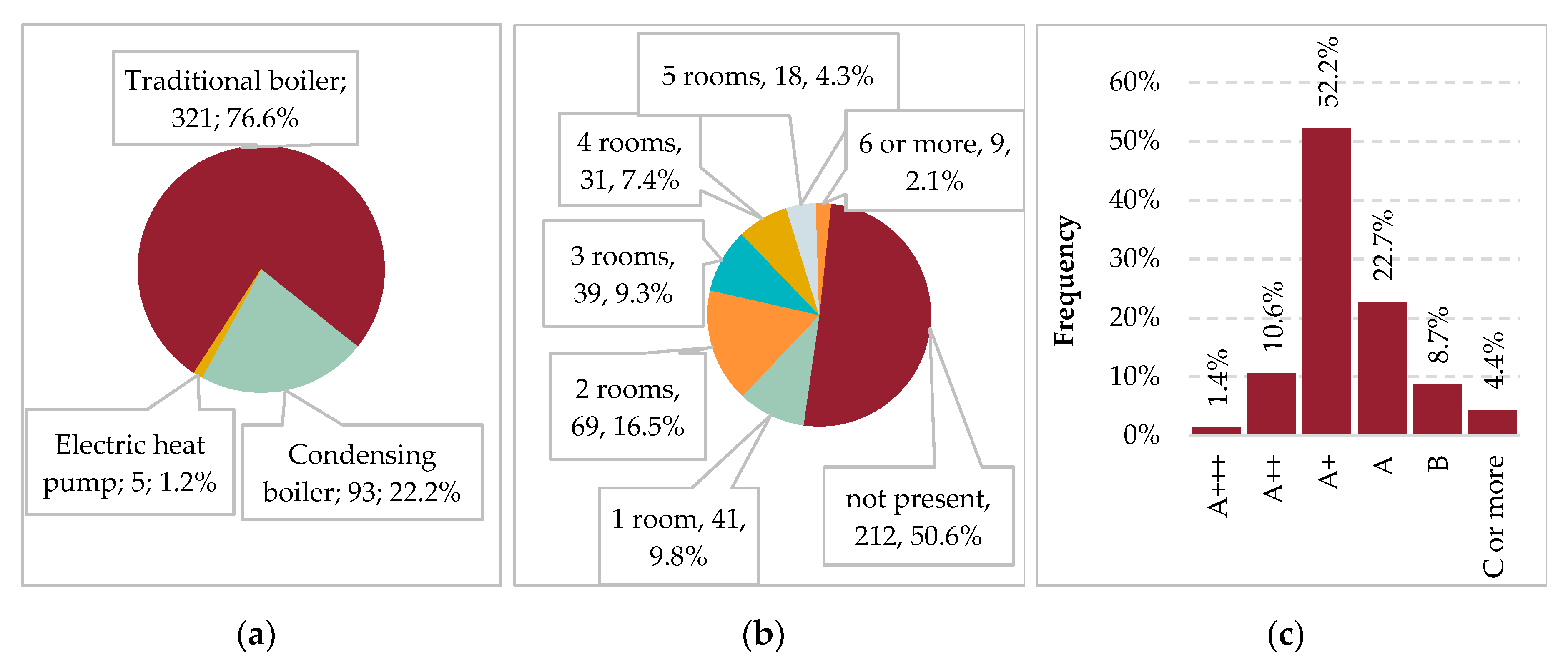
3.1. Dwellings Description and General Analysis on Consumptions Typology
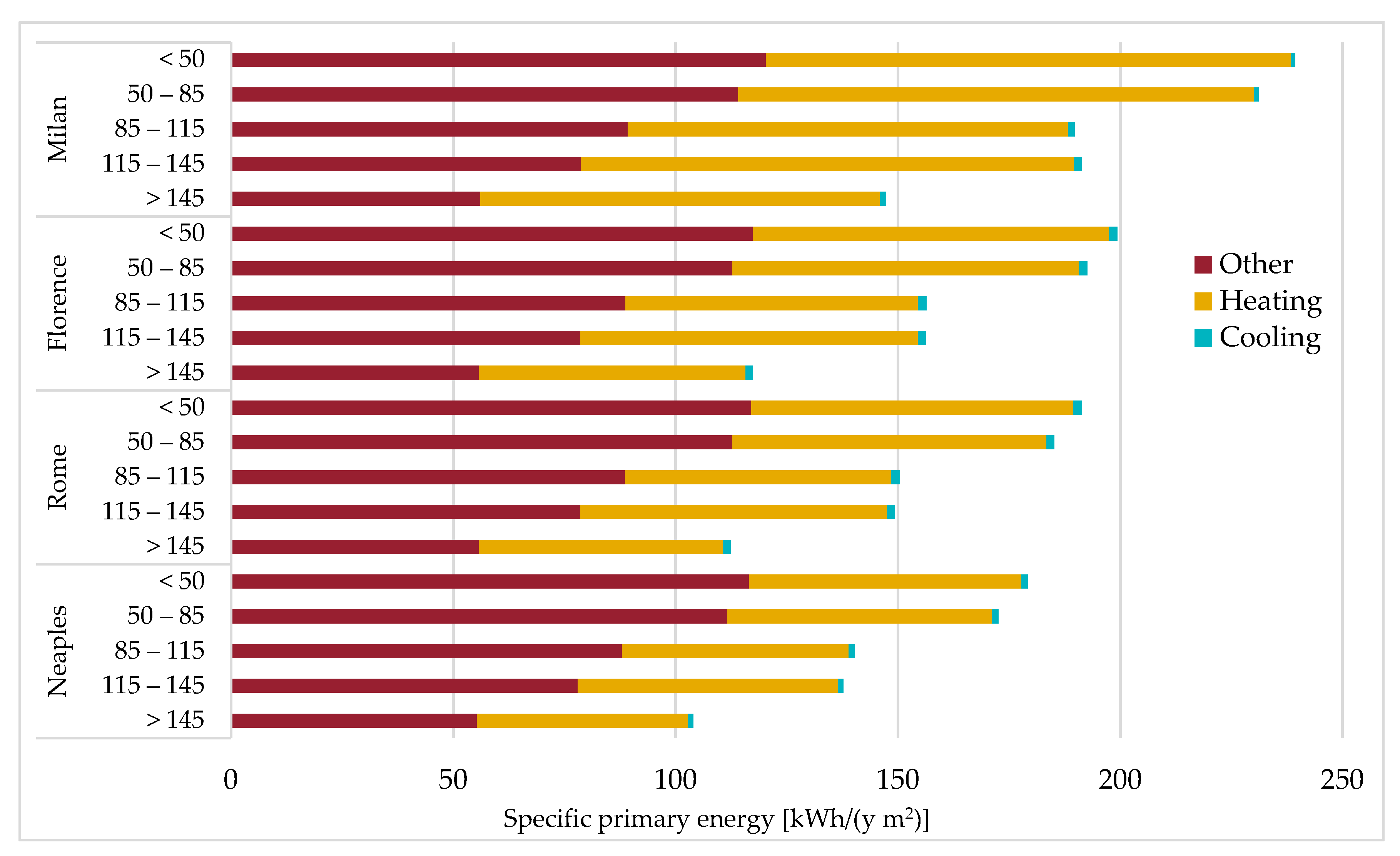
3.2. Energy Characterization of Dwellings in the Four Considered Cities
3.3. Changes in Heating and Cooling Energy Consumption Due to Temperature Enhancement
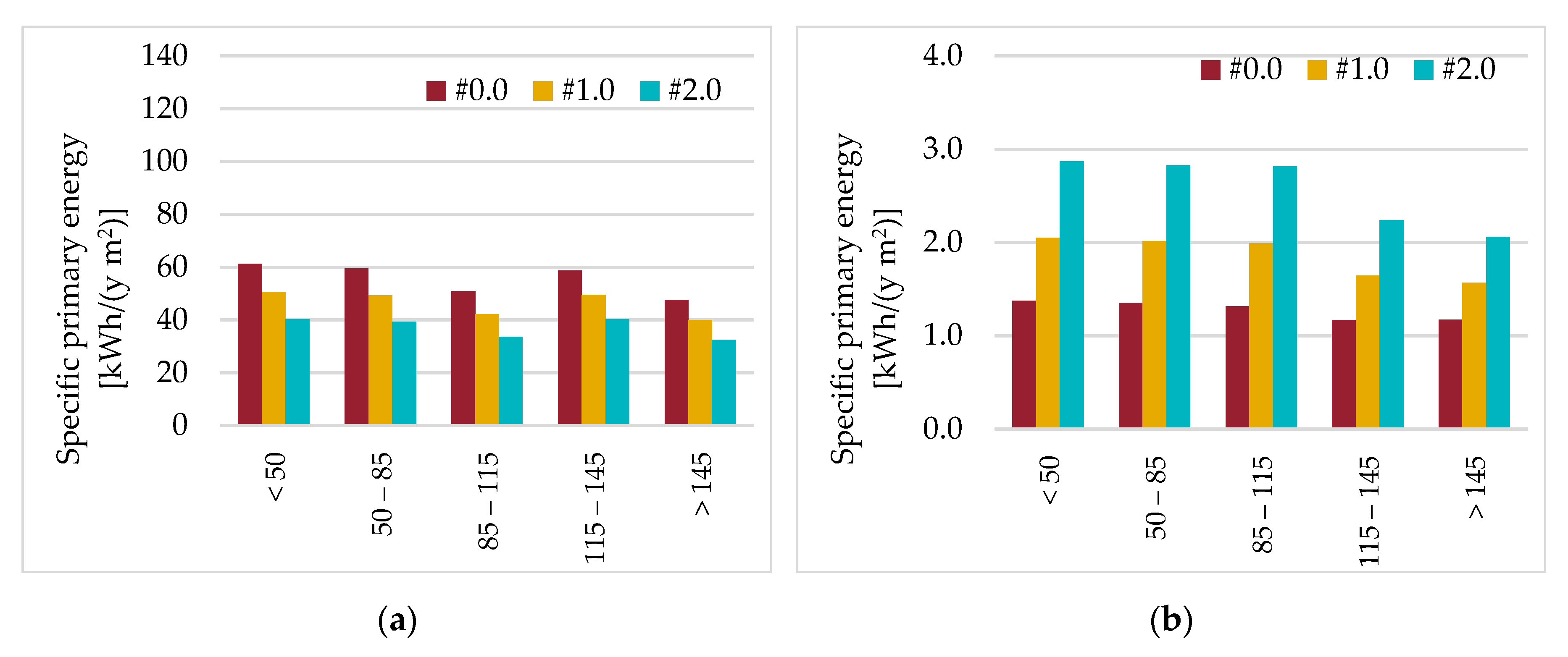
3.4. Change in Cooling Energy Consumption with the Addition of Air Conditioners
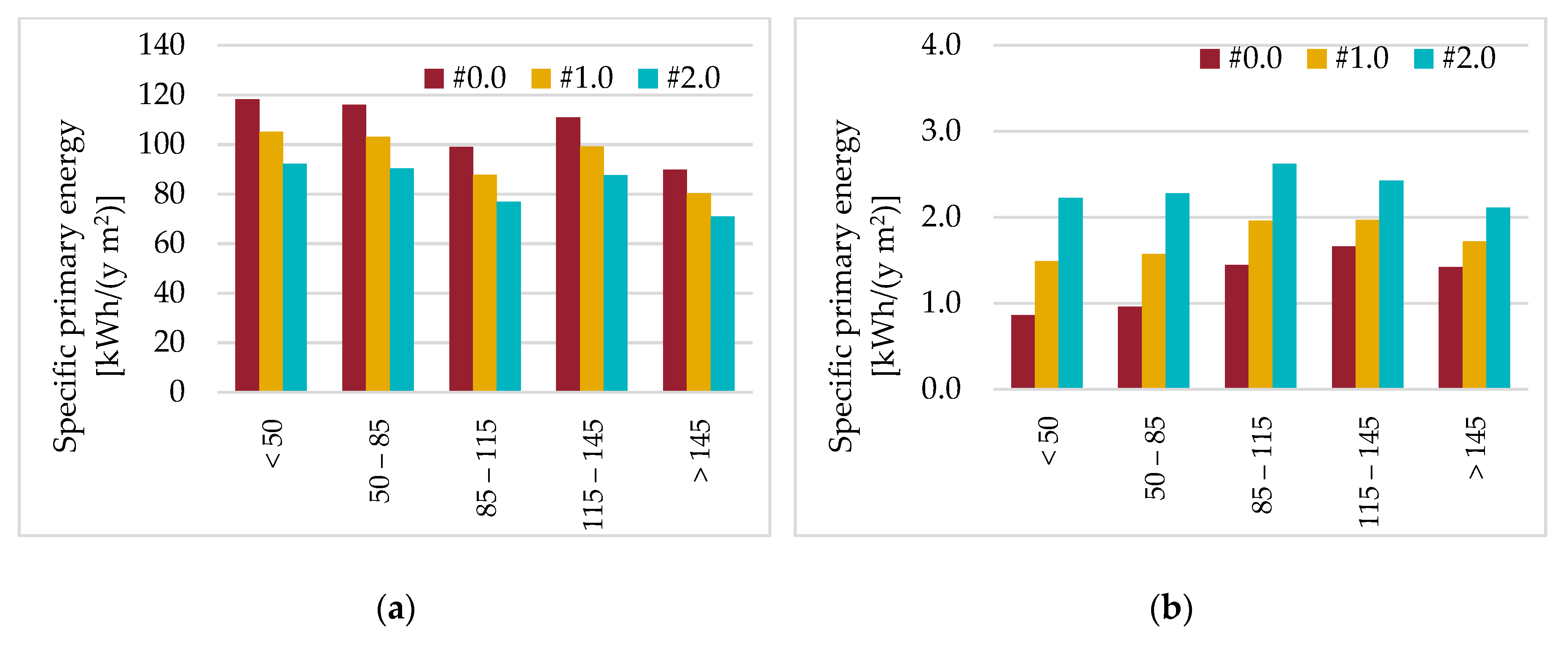
- For small houses in scenario #0.0 the consumption for cooling is equal to 0.9 kWh/ym2; in scenario #2.1 they are 5.9 kWh/ym2; in scenario #2.2 they are 6.0 kWh/ym2; percentage variations are equal to 556% and 567%, respectively;
- For large dwellings in scenario #0.0 the consumption for cooling is equal to 1.4 kWh/ym2; in scenario #2.1 they are 3.7 kWh/ym2; in scenario #2.2 they are equal to 4.1 kWh/ym2; the percentage variations rise up to 164% and 193%, respectively;
- On average in scenario #0.0 the consumption for cooling is equal to 1.3 kWh/ym2; in scenario #2.1 they are equal to 4.3 kWh/ym2; in scenario #2.2 they are 4.7 kWh/ym2; the relative variations are 231% and 262%, respectively.
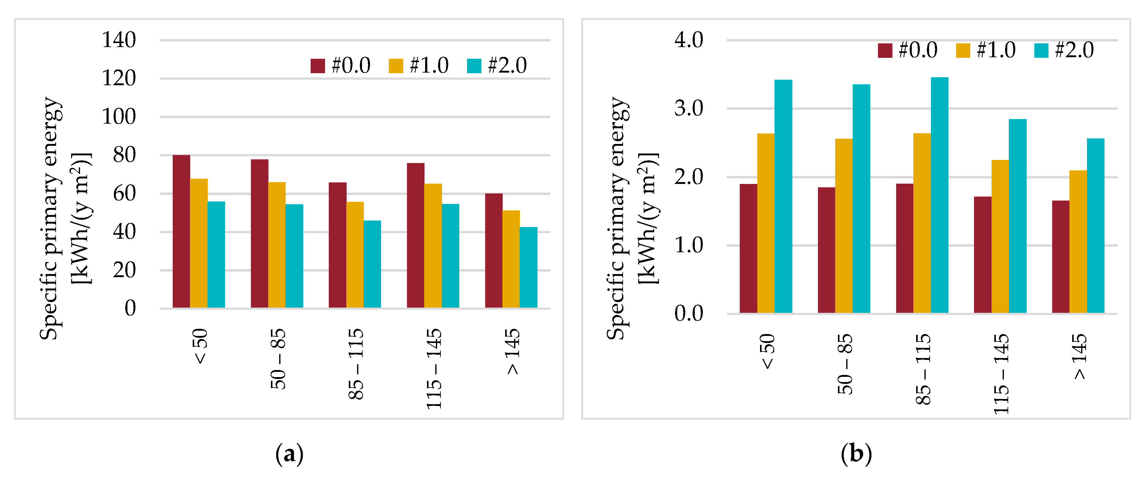
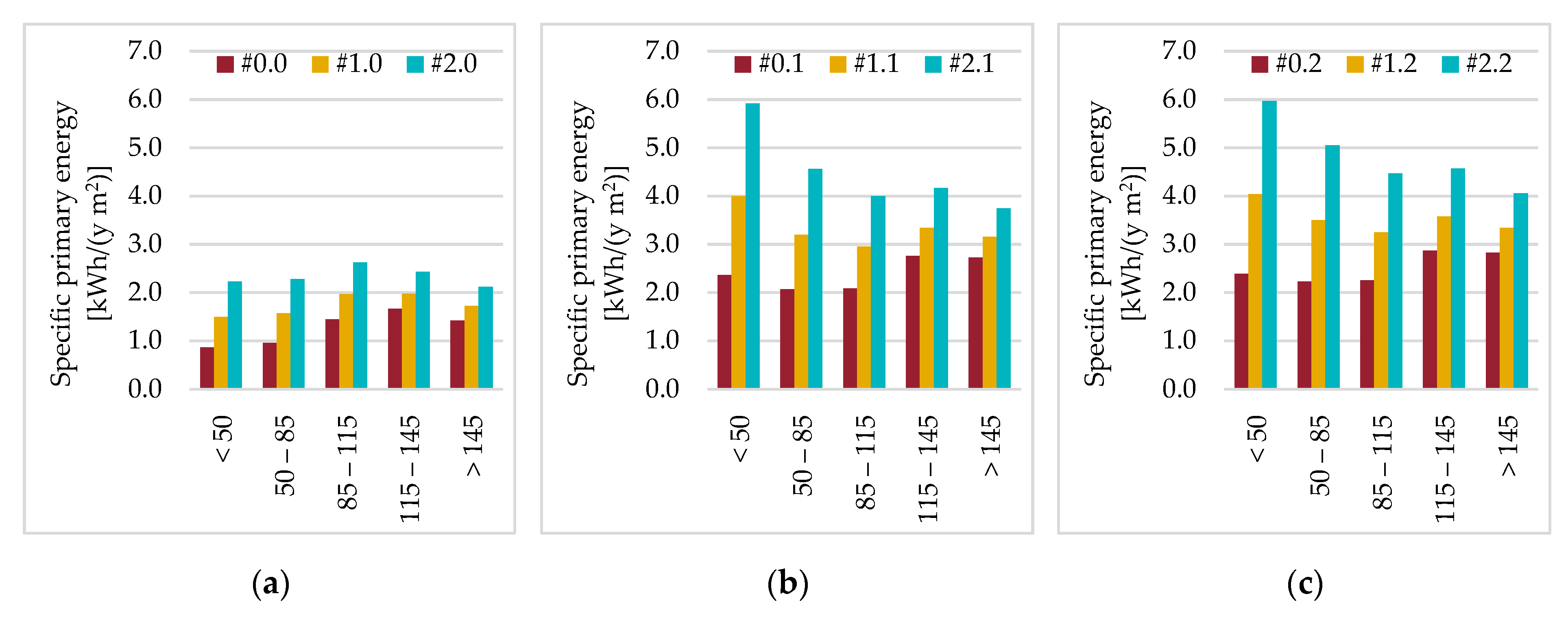
- For small dwellings in scenario #0.0 the consumption for cooling is 1.9 kWh/ym2; in scenario #2.1 they are equal to 9.2 kWh/ym2; in scenario #2.2 they are equal to 9.3 kWh/ym2; percentage variations are equal to 384% and 389%, respectively;
- For large dwellings in scenario #0.0 the consumption for cooling is equal to 1.7 kWh/ym2; in scenario #2.1 they are 4.4 kWh/ym2; in scenario #2.2 they are 4.9 kWh/ym2; percentage variations rise up to 159% and 188%, respectively;
- On average in scenario #0.0 the consumption for cooling is equal to 1.8 kWh/ym2; in scenario #2.1 they are 5.8 kWh/ym2; in scenario #2.2 they are equal to 6.4 kWh/ym2; relative variations are 222% and 256%.
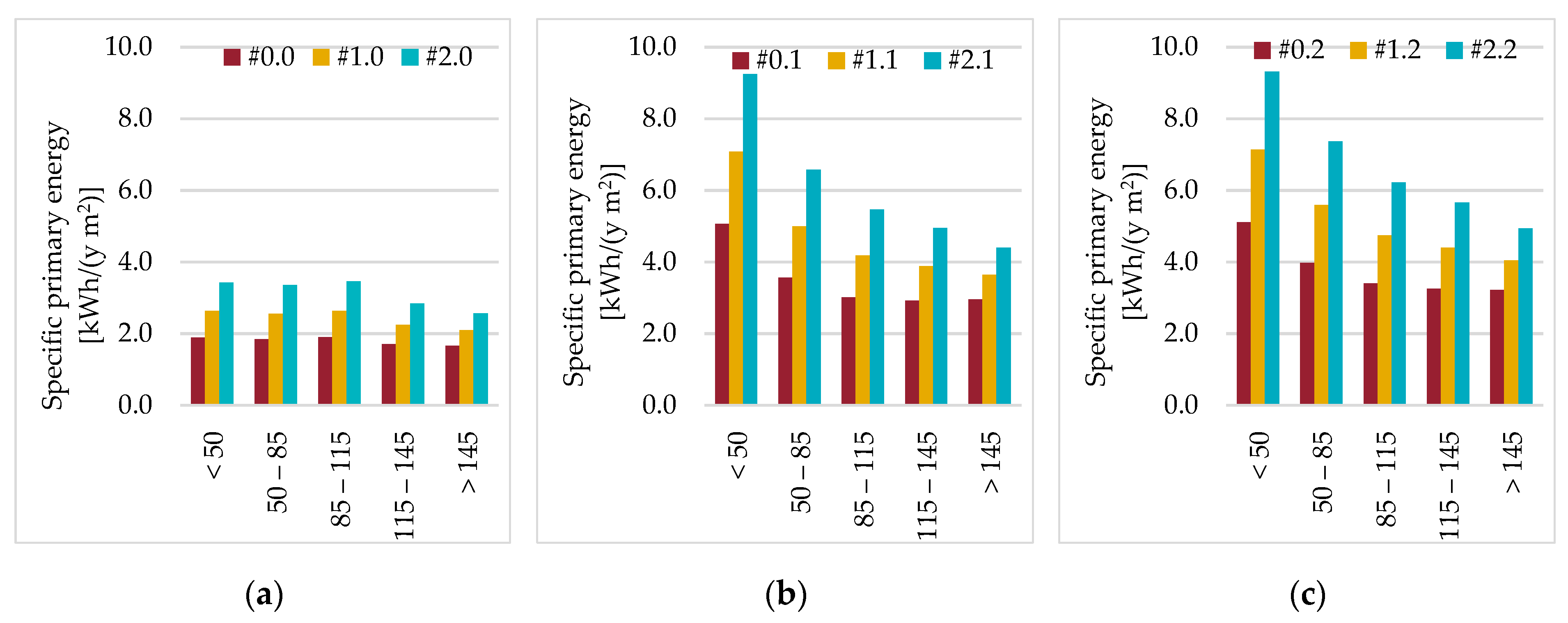
- For small dwellings in scenario #0.0 the consumption for cooling is 1.9 kWh/ym2; in scenario #2.1 they are 9.0 kWh/ym2; in scenario #2.2 they are 9.1 kWh/ym2; percentage variations are equal to 374% and 379%, respectively;
- For large dwellings in scenario #0.0 the consumption for cooling is 1.6 kWh/ym2; in scenario #2.1 they are 4.2 kWh/ym2; in scenario #2.2 they are 4.7 kWh/ym2; percentage variations rise up to 163% and 194%, respectively;
- On average in scenario #0.0 the consumption for cooling is equal to 1.8 kWh/ym2; in scenario #2.1 they are equal to 5.6 kWh/ym2; in scenario #2.2 they are 6.2 kWh/ym2; relative variations are 211% and 244%, respectively.
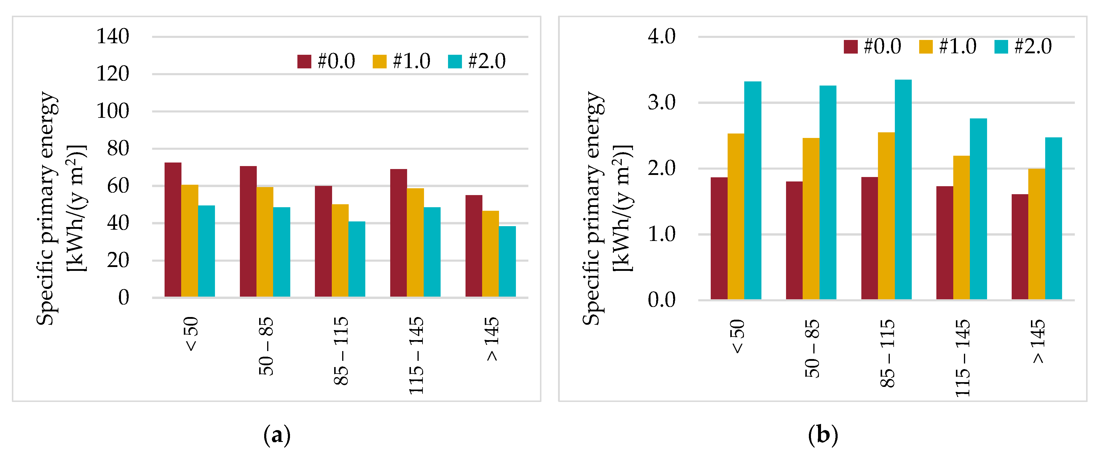
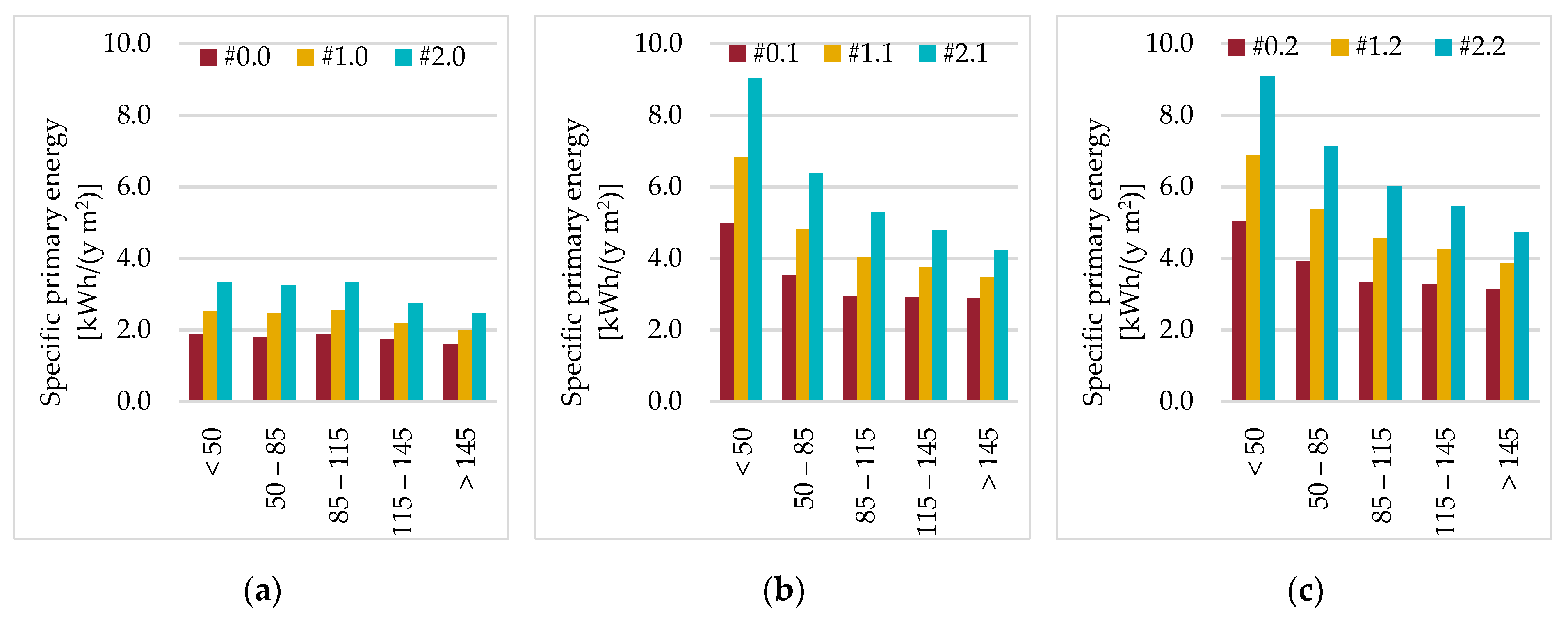
- For small houses in scenario #0.0 the consumption for cooling is 1.4 kWh/ym2; in scenario #2.1 they are equal to 7.7 kWh/ym2; in scenario #2.2 they are 7.8 kWh/ym2; percentage variations are equal to 450% and 457%, respectively;
- For large dwellings in scenario #0.0 the consumption for cooling is 1.2 kWh/ym2; in scenario #2.1 they are equal to 3.5 kWh/ym2; in scenario #2.2 they are equal to 3.9 kWh/ym2; percentage variations rise up to 192% and 225%;
- On average in scenario #0.0 the consumption for cooling is equal to 1.3 kWh/ym2; in scenario #2.1 they are 4.7 kWh/ym2; in scenario #2.2 they are equal to 5.2 kWh/ym2; relative variations are 262% and 300%.
3.5. Change in Overall Energy Consumption for Simulated Scenarios
3.6. Monthly Analysis of Cooling Consumption: Criticalities and Foreseeable Solutions
- There are typically multi-storey buildings in cities; consequently, the usable roof surface must be divided by the various floors;
- Not all roofs can be used for PV installation (surfaces already used, architectural constraints, poor irradiation conditions);
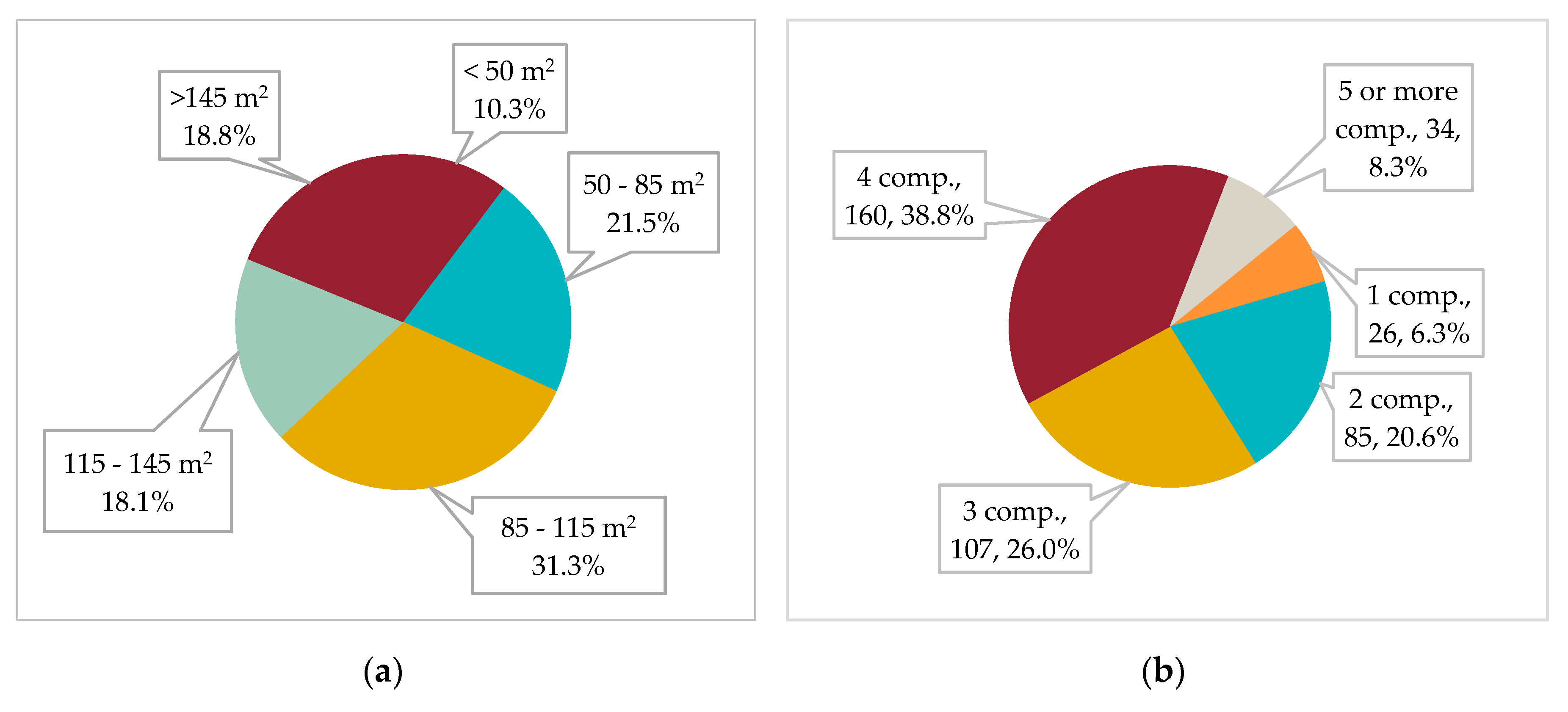
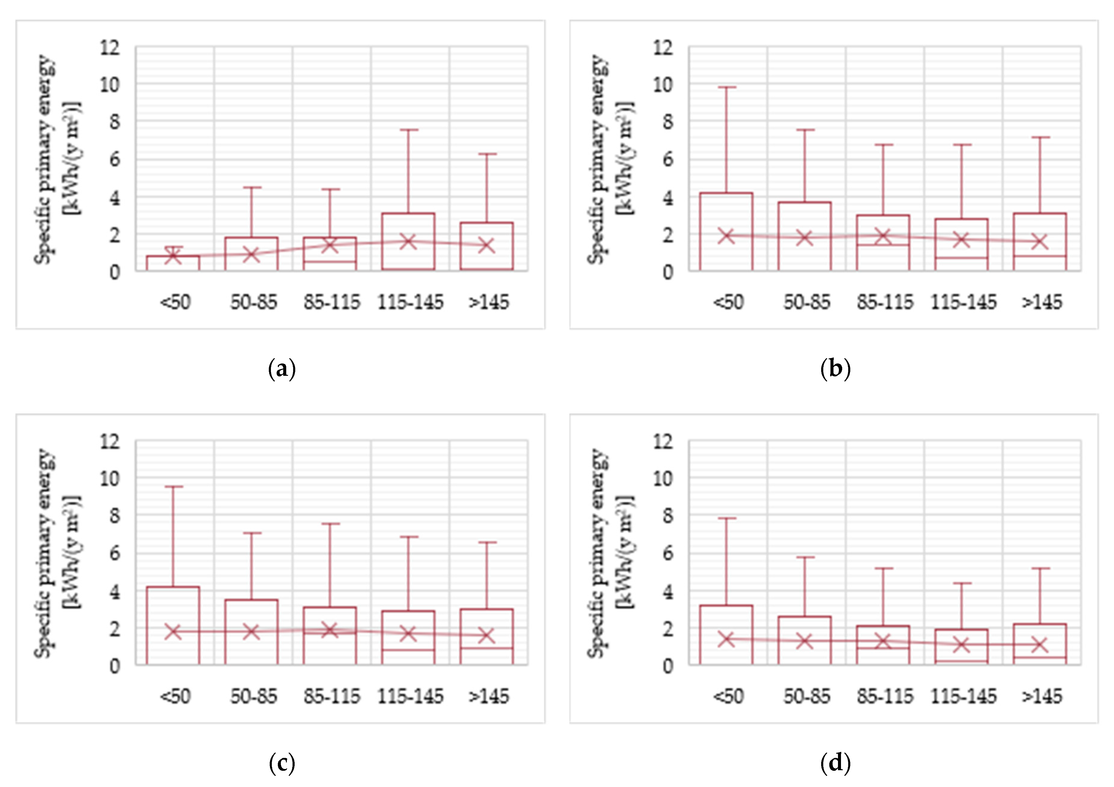
- The modern construction strategies lead to build new apartments characterised by a not wide floor surface (i.e., small < 50 m2; small-medium 50–85 m2), as well as by high specific consumptions for air conditioning, it being even double compared to the larger ones (see Figure 14, Figure 15, Figure 16 and Figure 17).
4. Conclusions
Author Contributions
Funding
Acknowledgments
Conflicts of Interest
Appendix A

Building Location
| Kitchen
|
References
- EUR-Lex—32018L2002—EN—EUR-Lex. Available online: https://eur-lex.europa.eu/legal-content/EN/TXT/?uri=uriserv%3AOJ.L_.2018.328.01.0210.01.ENG (accessed on 29 October 2019).
- EUR-Lex—32018L2001—EN—EUR-Lex. Available online: https://eur-lex.europa.eu/eli/dir/2018/2001/oj (accessed on 29 October 2019).
- EUR-Lex—32018L0844—EN—EUR-Lex. Available online: https://eur-lex.europa.eu/legal-content/EN/TXT/?toc=OJ%3AL%3A2018%3A156%3ATOC&uri=uriserv%3AOJ.L_.2018.156.01.0075.01.ENG (accessed on 29 October 2019).
- Paris Agreement. Climate Action. Available online: https://ec.europa.eu/clima/policies/international/negotiations/paris_en#tab-0-0 (accessed on 29 October 2019).
- IPCC—Intergovernmental Panel on Climate Change. Special Report on Global Warming of 1.5°C; IPCC—Intergovernmental Panel on Climate Change: Geneva, Switzerland, 2018. [Google Scholar]
- Kalvelage, K.; Passe, U.; Rabideau, S.; Takle, E.S. Changing climate: The effects on energy demand and human comfort. Energy Build. 2014, 76, 373–380. [Google Scholar] [CrossRef]
- Andrić, I.; Pina, A.; Ferrão, P.; Fournier, J.; Lacarrière, B.; Le Corre, O. The impact of climate change on building heat demand in different climate types. Energy Build. 2017, 149, 225–234. [Google Scholar] [CrossRef]
- Nik, V.M.; Mata, E.; Sasic Kalagasidis, A.; Scartezzini, J.-L. Effective and robust energy retrofitting measures for future climatic conditions—Reduced heating demand of Swedish households. Energy Build. 2016, 121, 176–187. [Google Scholar] [CrossRef]
- Van Hooff, T.; Blocken, B.; Timmermans, H.J.P.; Hensen, J.L.M. Analysis of the predicted effect of passive climate adaptation measures on energy demand for cooling and heating in a residential building. Energy 2016, 94, 811–820. [Google Scholar] [CrossRef]
- Eurostat Database—Eurostat. Available online: https://ec.europa.eu/eurostat/data/database (accessed on 4 April 2019).
- Morton, T.A.; Bretschneider, P.; Coley, D.; Kershaw, T. Building a better future: An exploration of beliefs about climate change and perceived need for adaptation within the building industry. Build. Environ. 2011, 46, 1151–1158. [Google Scholar] [CrossRef]
- Holmes, M.J.; Hacker, J.N. Climate change, thermal comfort and energy: Meeting the design challenges of the 21st century. Energy Build. 2007, 39, 802–814. [Google Scholar] [CrossRef]
- Crawley, D.B. Estimating the impacts of climate change and urbanization on building performance. J. Build. Perform. Simul. 2008, 1, 91–115. [Google Scholar] [CrossRef]
- Fazeli, R.; Davidsdottir, B.; Hallgrimsson, J.H. Climate Impact on Energy Demand for Space Heating in Iceland. Clim. Chang. Econ. 2016, 7, 1650004. [Google Scholar] [CrossRef]
- Jenkins, D.P.; Patidar, S.; Banfill, P.F.G.; Gibson, G.J. Probabilistic climate projections with dynamic building simulation: Predicting overheating in dwellings. Energy Build. 2011, 43, 1723–1731. [Google Scholar] [CrossRef]
- Berger, T.; Amann, C.; Formayer, H.; Korjenic, A.; Pospischal, B.; Neururer, C.; Smutny, R. Impacts of climate change upon cooling and heating energy demand of office buildings in Vienna, Austria. Energy Build. 2014, 80, 517–530. [Google Scholar] [CrossRef]
- Asimakopoulos, D.A.; Santamouris, M.; Farrou, I.; Laskari, M.; Saliari, M.; Zanis, G.; Giannakidis, G.; Tigas, K.; Kapsomenakis, J.; Douvis, C.; et al. Modelling the energy demand projection of the building sector in Greece in the 21st century. Energy Build. 2012, 49, 488–498. [Google Scholar] [CrossRef]
- Emmerling, J.; Tavoni, M. Exploration of the interactions between mitigation and solar radiation management in cooperative and non-cooperative international governance settings. Glob. Environ. Chang. 2018, 53, 244–251. [Google Scholar] [CrossRef]
- Perpiña Castillo, C.; Batista e Silva, F.; Lavalle, C. An assessment of the regional potential for solar power generation in EU-28. Energy Policy 2016, 88, 86–99. [Google Scholar] [CrossRef]
- Palmer, D.; Gottschalg, R.; Betts, T. The future scope of large-scale solar in the UK: Site suitability and target analysis. Renew. Energy 2019, 133, 1136–1146. [Google Scholar] [CrossRef]
- Giamalaki, M.; Tsoutsos, T. Sustainable siting of solar power installations in Mediterranean using a GIS/AHP approach. Renew. Energy 2019, 141, 64–75. [Google Scholar] [CrossRef]
- Biyik, E.; Araz, M.; Hepbasli, A.; Shahrestani, M.; Yao, R.; Shao, L.; Essah, E.; Oliveira, A.C.; del Caño, T.; Rico, E.; et al. A key review of building integrated photovoltaic (BIPV) systems. Eng. Sci. Technol. Int. J. 2017, 20, 833–858. [Google Scholar] [CrossRef]
- Saretta, E.; Caputo, P.; Frontini, F. A review study about energy renovation of building facades with BIPV in urban environment. Sustain. Cities Soc. 2019, 44, 343–355. [Google Scholar] [CrossRef]
- Overholm, H. Spreading the rooftop revolution: What policies enable solar-as-a-service? Energy Policy 2015, 84, 69–79. [Google Scholar] [CrossRef]
- Horváth, D.; Szabó, R.Z. Evolution of photovoltaic business models: Overcoming the main barriers of distributed energy deployment. Renew. Sustain. Energy Rev. 2018, 90, 623–635. [Google Scholar] [CrossRef]
- Augustine, P.; McGavisk, E. The next big thing in renewable energy: Shared solar. Electr. J. 2016, 29, 36–42. [Google Scholar] [CrossRef]
- Yildiz, Ö.; Rommel, J.; Debor, S.; Holstenkamp, L.; Mey, F.; Müller, J.R.; Radtke, J.; Rognli, J. Renewable energy cooperatives as gatekeepers or facilitators? Recent developments in Germany and a multidisciplinary research agenda. Energy Res. Soc. Sci. 2015, 6, 59–73. [Google Scholar] [CrossRef]
- Herbes, C.; Brummer, V.; Rognli, J.; Blazejewski, S.; Gericke, N. Responding to policy change: New business models for renewable energy cooperatives—Barriers perceived by cooperatives’ members. Energy Policy 2017, 109, 82–95. [Google Scholar] [CrossRef]
- Shimizu, T.; Kikuchi, Y.; Sugiyama, H.; Hirao, M. Design method for a local energy cooperative network using distributed energy technologies. Appl. Energy 2015, 154, 781–793. [Google Scholar] [CrossRef]
- Sifakis, N.; Savvakis, N.; Daras, T.; Tsoutsos, T. Analysis of the energy consumption behavior of European RES cooperative members. Energies 2019, 12, 970. [Google Scholar] [CrossRef]
- Simoes, S.G.; Dias, L.; Gouveia, J.P.; Seixas, J.; De Miglio, R.; Chiodi, A.; Gargiulo, M.; Long, G.; Giannakidis, G. INSMART—Insights on integrated modelling of EU cities energy system transition. Energy Strateg. Rev. 2018, 20, 150–155. [Google Scholar] [CrossRef]
- De Santoli, L.; Mancini, F.; Astiaso Garcia, D. A GIS-based model to assess electric energy consumptions and usable renewable energy potential in Lazio region at municipality scale. Sustain. Cities Soc. 2019, 46, 101413. [Google Scholar] [CrossRef]
- Nastasi, B.; Lo Basso, G.; Astiaso Garcia, D.; Cumo, F.; de Santoli, L. Power-to-gas leverage effect on power-to-heat application for urban renewable thermal energy systems. Int. J. Hydrogen Energy 2018, 43, 23076–23090. [Google Scholar] [CrossRef]
- Groppi, D.; de Santoli, L.; Cumo, F.; Astiaso Garcia, D. A GIS-based model to assess buildings energy consumption and usable solar energy potential in urban areas. Sustain. Cities Soc. 2018, 40, 546–558. [Google Scholar] [CrossRef]
- Roversi, R.; Cumo, F.; D’angelo, A.; Pennacchia, E.; Piras, G. Feasibility of municipal waste reuse for building envelopes for near zero-energy buildings. In Proceedings of the WIT Transactions on Ecology and the Environment; WIT Press: Southampton, UK, 2017; Volume 224, pp. 115–125. [Google Scholar]
- Lombardi, M.; Laiola, E.; Tricase, C.; Rana, R. Toward urban environmental sustainability: The carbon footprint of Foggia’s municipality. J. Clean. Prod. 2018, 186, 534–543. [Google Scholar] [CrossRef]
- Astiaso Garcia, D.; Cumo, F.; Pennacchia, E.; Stefanini Pennucci, V.; Piras, G.; De Notti, V.; Roversi, R. Assessment of a urban sustainability and life quality index for elderly. Int. J. Sustain. Dev. Plan. 2017, 12, 908–921. [Google Scholar] [CrossRef]
- Cumo, F.; Curreli, F.R.; Pennacchia, E.; Piras, G.; Roversi, R. Enhancing the urban quality of life: A case study of a coastal city in the metropolitan area of rome. In WIT Transactions on The Built Environment; WIT Press: Southampton, UK, 2017; Volume 170, pp. 127–137. [Google Scholar]
- Mancini, F.; Lo Basso, G.; De Santoli, L. Energy Use in Residential Buildings: Characterisation for Identifying Flexible Loads by Means of a Questionnaire Survey. Energies 2019, 12, 2055. [Google Scholar] [CrossRef]
- Mancini, F.; Nastasi, B. Energy Retrofitting Effects on the Energy Flexibility of Dwellings. Energies 2019, 12, 2788. [Google Scholar] [CrossRef]
- Mancini, F.; Lo Basso, G.; de Santoli, L. Energy Use in Residential Buildings: Impact of Building Automation Control Systems on Energy Performance and Flexibility. Energies 2019, 12, 2896. [Google Scholar] [CrossRef]
- Mata, É.; Kalagasidis, A.S.; Johnsson, F. A modelling strategy for energy, carbon, and cost assessments of building stocks. Energy Build. 2013, 56, 100–108. [Google Scholar] [CrossRef]
- Andrić, I.; Gomes, N.; Pina, A.; Ferrão, P.; Fournier, J.; Lacarrière, B.; Le Corre, O. Modeling the long-term effect of climate change on building heat demand: Case study on a district level. Energy Build. 2016, 126, 77–93. [Google Scholar] [CrossRef]
- Cui, Y.; Yan, D.; Hong, T.; Xiao, C.; Luo, X.; Zhang, Q. Comparison of typical year and multiyear building simulations using a 55-year actual weather data set from China. Appl. Energy 2017, 195, 890–904. [Google Scholar] [CrossRef]
- ASHRAE. Handbook—Fundamentals (SI Edition); ASHRAE: Atlanta, GA, USA, 2017; ISBN 6785392187. [Google Scholar]
- UNI Italian Standard UNI 10349-1:2016—Heating and Cooling of Buildings—Climatic Data. Available online: http://store.uni.com/catalogo/uni-10349-1-2016?___store=en&josso_back_to=http%3A%2F%2Fstore.uni.com%2Fjosso-security-check.php&josso_cmd=login_optional&josso_partnerapp_host=store.uni.com&___from_store=it (accessed on 12 October 2019).
- Archivio Meteo Storico—ILMETEO.it. Available online: https://www.ilmeteo.it/portale/archivio-meteo (accessed on 12 October 2019).
- Chiabrando, R.; Fabrizio, E.; Garnero, G. The territorial and landscape impacts of photovoltaic systems: Definition of impacts and assessment of the glare risk. Renew. Sustain. Energy Rev. 2009, 13, 2441–2451. [Google Scholar] [CrossRef]
- Mauro, G.; Lughi, V. Mapping land use impact of photovoltaic farms via crowdsourcing in the Province of Lecce (Southeastern Italy). Sol. Energy 2017, 155, 434–444. [Google Scholar] [CrossRef]
- JRC Photovoltaic Geographical Information System (PVGIS)—European Commission. Available online: https://re.jrc.ec.europa.eu/pvg_tools/en/tools.html#PVP (accessed on 29 October 2019).
- ISTAT Italian National Institute of Statistics Edifici Residenziali. Available online: http://dati-censimentopopolazione.istat.it/Index.aspx?DataSetCode=DICA_EDIFICIRES (accessed on 4 April 2019).
- De Santoli, L.; Mancini, F.; Basso, G.L. Analysis on the Potential of an Energy Aggregator for Domestic Users in the Italian Electricity System; AIP Publishing LLC: Melville, NY, USA, 2019; p. 020062. [Google Scholar]
- ISTAT Italian National Institute of Statistics. I Consumi Energetici Delle Famiglie; ISTAT Italian National Institute of Statistics: Rome, Italy, 2014. [Google Scholar]
- Dati Statistici. Available online: http://www.terna.it/SistemaElettrico/StatisticheePrevisioni/DatiStatistici.aspx (accessed on 11 April 2019).


| # | Climate Data | System Equipment |
|---|---|---|
| #0.0 | Italian Standard UNI 10349 | Existing equipment |
| #0.1 | Existing equipment + 1 air conditioner | |
| #0.2 | Existing equipment + 2 air conditioners | |
| #1.0 | Italian Standard UNI 10349 + 1.0 °C | Existing equipment |
| #1.1 | Existing equipment + 1 air conditioner | |
| #1.2 | Existing equipment + 2 air conditioners | |
| #2.0 | Italian Standard UNI 10349 + 2.0 °C | Existing equipment |
| #2.1 | Existing equipment + 1 air conditioner | |
| #2.2 | Existing equipment + 2 air conditioners |
| Building Construction Year | N° and Fraction | Retrofitted Building Components | |||
|---|---|---|---|---|---|
| Walls | Roofs | Floors | Windows | ||
| before 1919 | 12 (2.9%) | 0 (0%) | 0 (0%) | 0 (0%) | 5 (41.7%) |
| 1919–1945 | 42 (10%) | 2 (4.8%) | 2 (4.8%) | 3 (7.1%) | 29 (69%) |
| 1946–1961 | 59 (14.1%) | 6 (10.2%) | 8 (13.6%) | 1 (1.7%) | 46 (78%) |
| 1962–1971 | 63 (15%) | 8 (12.7%) | 7 (11.1%) | 3 (4.8%) | 29 (46%) |
| 1972–1981 | 88 (21%) | 13 (14.8%) | 13 (14.8%) | 5 (5.7%) | 44 (50%) |
| 1982–1991 | 63 (15%) | 6 (9.5%) | 7 (11.1%) | 4 (6.3%) | 27 (42.9%) |
| 1991–2005 | 75 (17.9%) | 16 (21.3%) | 14 (18.7%) | 9 (12%) | 13 (17.3%) |
| 2006–2008 | 2 (0.5%) | 0 (0%) | 0 (0%) | 0 (0%) | 0 (0%) |
| 2008–2010 | 6 (1.4%) | 2 (33.3%) | 1 (16.7%) | 0 (0%) | 2 (33.3%) |
| 2010–2015 | 8 (1.9%) | 4 (50%) | 4 (50%) | 3 (37.5%) | 2 (25%) |
| after 2015 | 1 (0.2%) | 0 (0%) | 0 (0%) | 0 (0%) | 0 (0%) |
| Total | 419 (100%) | 57 (13.6%) | 56 (13.4%) | 28 (6.7%) | 197 (47%) |
| City | Scenario | <50 m2 | 50–85 m2 | 85–115 m2 | 115–145 m2 | >145 m2 | |||||
|---|---|---|---|---|---|---|---|---|---|---|---|
| (kWh/ym2) | (%) | (kWh/ym2) | (%) | (kWh/ym2) | (%) | (kWh/ym2) | (%) | (kWh/ym2) | (%) | ||
| Milan | #0.0 | 239.4 | 231.1 | 189.7 | 191.4 | 147.4 | |||||
| #0.1 | 240.9 | 0.6% | 232.2 | 0.5% | 190.4 | 0.3% | 192.4 | 0.6% | 148.7 | 0.9% | |
| #0.2 | 240.9 | 0.6% | 232.4 | 0.5% | 190.5 | 0.4% | 192.6 | 0.6% | 148.8 | 1.0% | |
| #1.0 | 226.6 | −5.3% | 218.5 | −5.5% | 178.9 | −5.7% | 179.8 | −6.0% | 138.1 | −6.3% | |
| #1.1 | 229.1 | −4.3% | 220.1 | −4.8% | 179.9 | −5.2% | 181.2 | −5.3% | 139.5 | −5.3% | |
| #1.2 | 229.2 | −4.3% | 220.4 | −4.6% | 180.2 | −5.0% | 181.4 | −5.2% | 139.7 | −5.2% | |
| #2.0 | 214.2 | −10.5% | 206.2 | −10.8% | 168.5 | −11.2% | 168.7 | −11.9% | 129.0 | −12.5% | |
| #2.1 | 217.9 | −9.0% | 208.5 | −9.8% | 169.9 | −10.4% | 170.4 | −11.0% | 130.6 | −11.4% | |
| #2.2 | 217.9 | −9.0% | 209.0 | −9.6% | 170.4 | −10.2% | 170.8 | −10.7% | 130.9 | −11.2% | |
| Florence | #0.0 | 199.3 | −16.7% | 192.6 | −16.7% | 156.5 | −17.5% | 156.2 | −18.4% | 117.4 | −20.3% |
| #0.1 | 202.5 | −15.4% | 194.3 | −15.9% | 157.6 | −16.9% | 157.4 | −17.7% | 118.7 | −19.4% | |
| #0.2 | 202.5 | −15.4% | 194.7 | −15.8% | 158.0 | −16.7% | 157.8 | −17.5% | 119.0 | −19.3% | |
| #1.0 | 187.5 | −21.7% | 181.1 | −21.6% | 146.8 | −22.6% | 145.9 | −23.8% | 109.0 | −26.0% | |
| #1.1 | 191.9 | −19.8% | 183.6 | −20.6% | 148.4 | −21.8% | 147.5 | −22.9% | 110.6 | −25.0% | |
| #1.2 | 192.0 | −19.8% | 184.1 | −20.3% | 148.9 | −21.5% | 148.0 | −22.6% | 111.0 | −24.7% | |
| #2.0 | 176.0 | −26.5% | 170.1 | −26.4% | 137.6 | −27.4% | 135.7 | −29.1% | 100.7 | −31.6% | |
| #2.1 | 181.8 | −24.0% | 173.3 | −25.0% | 139.7 | −26.4% | 137.8 | −28.0% | 102.6 | −30.4% | |
| #2.2 | 181.9 | −24.0% | 174.1 | −24.7% | 140.4 | −26.0% | 138.5 | −27.6% | 103.1 | −30.0% | |
| Rome | #0.0 | 191.4 | −20.0% | 185.2 | −19.9% | 150.4 | −20.7% | 149.3 | −22.0% | 112.4 | −23.8% |
| #0.1 | 194.5 | −18.7% | 186.9 | −19.1% | 151.5 | −20.1% | 150.5 | −21.3% | 113.6 | −22.9% | |
| #0.2 | 194.6 | −18.7% | 187.3 | −18.9% | 151.9 | −19.9% | 150.9 | −21.2% | 113.9 | −22.7% | |
| #1.0 | 179.9 | −24.8% | 174.2 | −24.6% | 141.2 | −25.6% | 139.2 | −27.2% | 104.2 | −29.3% | |
| #1.1 | 184.2 | −23.1% | 176.6 | −23.6% | 142.6 | −24.8% | 140.8 | −26.4% | 105.7 | −28.3% | |
| #1.2 | 184.2 | −23.0% | 177.1 | −23.3% | 143.2 | −24.5% | 141.3 | −26.2% | 106.1 | −28.0% | |
| #2.0 | 169.3 | −29.3% | 163.9 | −29.1% | 132.5 | −30.1% | 129.6 | −32.3% | 96.4 | −34.6% | |
| #2.1 | 175.0 | −26.9% | 167.0 | −27.7% | 134.5 | −29.1% | 131.6 | −31.2% | 98.1 | −33.4% | |
| #2.2 | 175.0 | −26.9% | 167.8 | −27.4% | 135.2 | −28.7% | 132.3 | −30.9% | 98.7 | −33.1% | |
| Naples | #0.0 | 179.2 | −25.1% | 172.6 | −25.3% | 140.2 | −26.1% | 137.8 | −28.0% | 104.0 | −29.4% |
| #0.1 | 181.5 | −24.2% | 173.8 | −24.8% | 141.0 | −25.7% | 138.6 | −27.6% | 105.0 | −28.8% | |
| #0.2 | 181.6 | −24.1% | 174.1 | −24.7% | 141.3 | −25.5% | 138.8 | −27.4% | 105.2 | −28.6% | |
| #1.0 | 168.9 | −29.4% | 162.8 | −29.5% | 132.0 | −30.4% | 128.9 | −32.6% | 96.8 | −34.3% | |
| #1.1 | 172.4 | −28.0% | 164.7 | −28.7% | 133.2 | −29.8% | 130.1 | −32.0% | 97.9 | −33.6% | |
| #1.2 | 172.4 | −28.0% | 165.1 | −28.5% | 133.6 | −29.6% | 130.5 | −31.8% | 98.2 | −33.4% | |
| #2.0 | 159.1 | −33.5% | 153.4 | −33.6% | 124.0 | −34.6% | 120.2 | −37.2% | 89.7 | −39.1% | |
| #2.1 | 164.0 | −31.5% | 156.0 | −32.5% | 125.7 | −33.8% | 121.9 | −36.3% | 91.1 | −38.2% | |
| #2.2 | 164.0 | −31.5% | 156.6 | −32.2% | 126.3 | −33.4% | 122.5 | −36.0% | 91.5 | −37.9% | |
| City | Scenario | June | July | August | September |
|---|---|---|---|---|---|
| Milan | #0.1 | 0.7% | 7.2% | 8.4% | 0.4% |
| #0.2 | 0.9% | 9.6% | 11.1% | 0.4% | |
| #1.0 | 2.3% | 5.3% | 5.2% | 0.6% | |
| #1.1 | 4.4% | 16.4% | 17.4% | 1.4% | |
| #1.2 | 5.1% | 20.1% | 21.5% | 1.6% | |
| #2.0 | 6.4% | 10.8% | 10.5% | 2.5% | |
| #2.1 | 11.5% | 25.8% | 26.7% | 4.6% | |
| #2.2 | 13.1% | 30.8% | 32.0% | 5.2% | |
| Florence | #0.1 | 3.1% | 10.7% | 9.0% | 0.3% |
| #0.2 | 4.1% | 14.3% | 12.0% | 0.3% | |
| #1.0 | 4.5% | 5.1% | 51% | 0.1% | |
| #1.1 | 10.9% | 19.5% | 17.9% | 0.4% | |
| #1.2 | 13.0% | 24.3% | 22.2% | 0.4% | |
| #2.0 | 10.1% | 10.2% | 10.4% | 0.4% | |
| #2.1 | 20.4% | 28.4% | 27.1% | 0.9% | |
| #2.2 | 23.8% | 34.5% | 32.6% | 1.0% | |
| Rome | #0.1 | 0.7% | 10.3% | 11.2% | 0.3% |
| #0.2 | 0.9% | 13.8% | 14.9% | 0.4% | |
| #1.0 | 2.2% | 5.3% | 5.1% | 0.6% | |
| #1.1 | 4.4% | 19.5% | 20.0% | 1.3% | |
| #1.2 | 5.0% | 24.3% | 24.9% | 1.5% | |
| #2.0 | 6.2% | 10.5% | 10.2% | 2.3% | |
| #2.1 | 11.2% | 28.6% | 28.8% | 4.2% | |
| #2.2 | 12.9% | 34.6% | 35.0% | 4.8% | |
| Naples | #0.1 | 0.7% | 7.2% | 8.4% | 0.4% |
| #0.2 | 0.9% | 9.6% | 11.1% | 0.4% | |
| #1.0 | 2.3% | 5.3% | 5.2% | 0.6% | |
| #1.1 | 4.4% | 16.4% | 17.4% | 1.4% | |
| #1.2 | 5.1% | 20.1% | 21.5% | 1.6% | |
| #2.0 | 6.4% | 10.8% | 10.5% | 2.5% | |
| #2.1 | 11.5% | 25.8% | 26.7% | 4.6% | |
| #2.2 | 13.1% | 30.8% | 32.0% | 5.2% |
| City | Scenario | June | July | August | September |
|---|---|---|---|---|---|
| Milan | #0.1 | 0.2% | 1.3% | 0.9% | 0.1% |
| #0.2 | 0.3% | 1.8% | 1.2% | 0.1% | |
| #1.0 | 0.7% | 1.4% | 1.1% | 0.0% | |
| #1.1 | 1.3% | 3.7% | 2.9% | 0.1% | |
| #1.2 | 1.5% | 4.5% | 3.4% | 0.1% | |
| #2.0 | 1.8% | 2.9% | 2.4% | 0.0% | |
| #2.1 | 3.3% | 6.3% | 5.1% | 0.1% | |
| #2.2 | 3.7% | 7.4% | 6.0% | 0.1% | |
| Florence | #0.1 | 0.8% | 2.9% | 2.4% | 0.1% |
| #0.2 | 1.1% | 3.9% | 3.2% | 0.1% | |
| #1.0 | 1.2% | 1.4% | 1.4% | 0.0% | |
| #1.1 | 2.9% | 5.3% | 4.8% | 0.1% | |
| #1.2 | 3.4% | 6.6% | 6.0% | 0.1% | |
| #2.0 | 2.6% | 2.8% | 2.8% | 0.1% | |
| #2.1 | 5.3% | 7.7% | 7.3% | 0.2% | |
| #2.2 | 6.2% | 9.3% | 8.8% | 0.3% | |
| Rome | #0.1 | 0.2% | 2.6% | 2.9% | 0.1% |
| #0.2 | 0.2% | 3.5% | 3.9% | 0.1% | |
| #1.0 | 0.5% | 1.3% | 1.3% | 0.2% | |
| #1.1 | 1.0% | 4.9% | 5.3% | 0.4% | |
| #1.2 | 1.2% | 6.2% | 6.6% | 0.4% | |
| #2.0 | 1.4% | 2.7% | 2.7% | 0.6% | |
| #2.1 | 2.6% | 7.2% | 7.6% | 1.1% | |
| #2.2 | 3.0% | 8.8% | 9.3% | 1.3% | |
| Naples | #0.1 | 0.2% | 1.7% | 2.1% | 0.1% |
| #0.2 | 0.2% | 2.3% | 2.8% | 0.1% | |
| #1.0 | 0.5% | 1.3% | 1.3% | 0.2% | |
| #1.1 | 1.0% | 3.9% | 4.3% | 0.4% | |
| #1.2 | 1.1% | 4.8% | 5.3% | 0.4% | |
| #2.0 | 1.4% | 2.6% | 2.6% | 0.6% | |
| #2.1 | 2.6% | 6.2% | 6.6% | 1.2% | |
| #2.2 | 2.9% | 7.4% | 7.9% | 1.3% |
© 2020 by the authors. Licensee MDPI, Basel, Switzerland. This article is an open access article distributed under the terms and conditions of the Creative Commons Attribution (CC BY) license (http://creativecommons.org/licenses/by/4.0/).
Share and Cite
Mancini, F.; Lo Basso, G. How Climate Change Affects the Building Energy Consumptions Due to Cooling, Heating, and Electricity Demands of Italian Residential Sector. Energies 2020, 13, 410. https://doi.org/10.3390/en13020410
Mancini F, Lo Basso G. How Climate Change Affects the Building Energy Consumptions Due to Cooling, Heating, and Electricity Demands of Italian Residential Sector. Energies. 2020; 13(2):410. https://doi.org/10.3390/en13020410
Chicago/Turabian StyleMancini, Francesco, and Gianluigi Lo Basso. 2020. "How Climate Change Affects the Building Energy Consumptions Due to Cooling, Heating, and Electricity Demands of Italian Residential Sector" Energies 13, no. 2: 410. https://doi.org/10.3390/en13020410
APA StyleMancini, F., & Lo Basso, G. (2020). How Climate Change Affects the Building Energy Consumptions Due to Cooling, Heating, and Electricity Demands of Italian Residential Sector. Energies, 13(2), 410. https://doi.org/10.3390/en13020410