Planning of Distributed Energy Storage Systems in μGrids Accounting for Voltage Dips


Abstract
1. Introduction
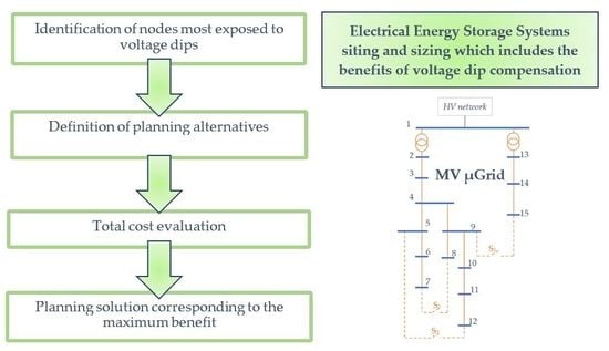
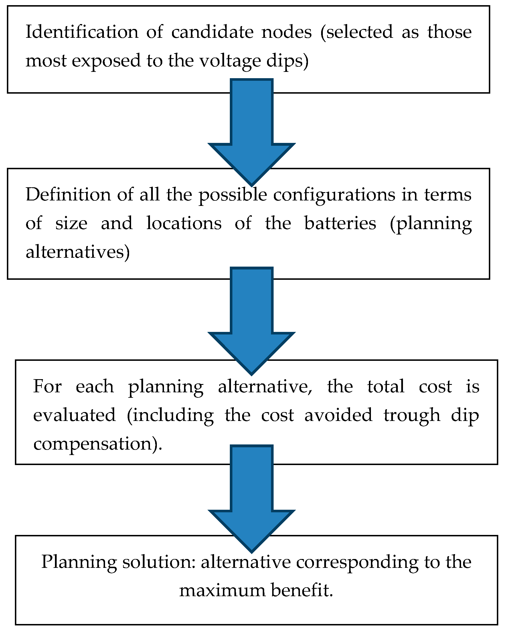
2. Problem Formulation
3. Identification of the Set of Buses Most Exposed to the Voltage Dips
4. Total Cost Evaluation
4.1. Installation Cost
4.2. Replacement Cost
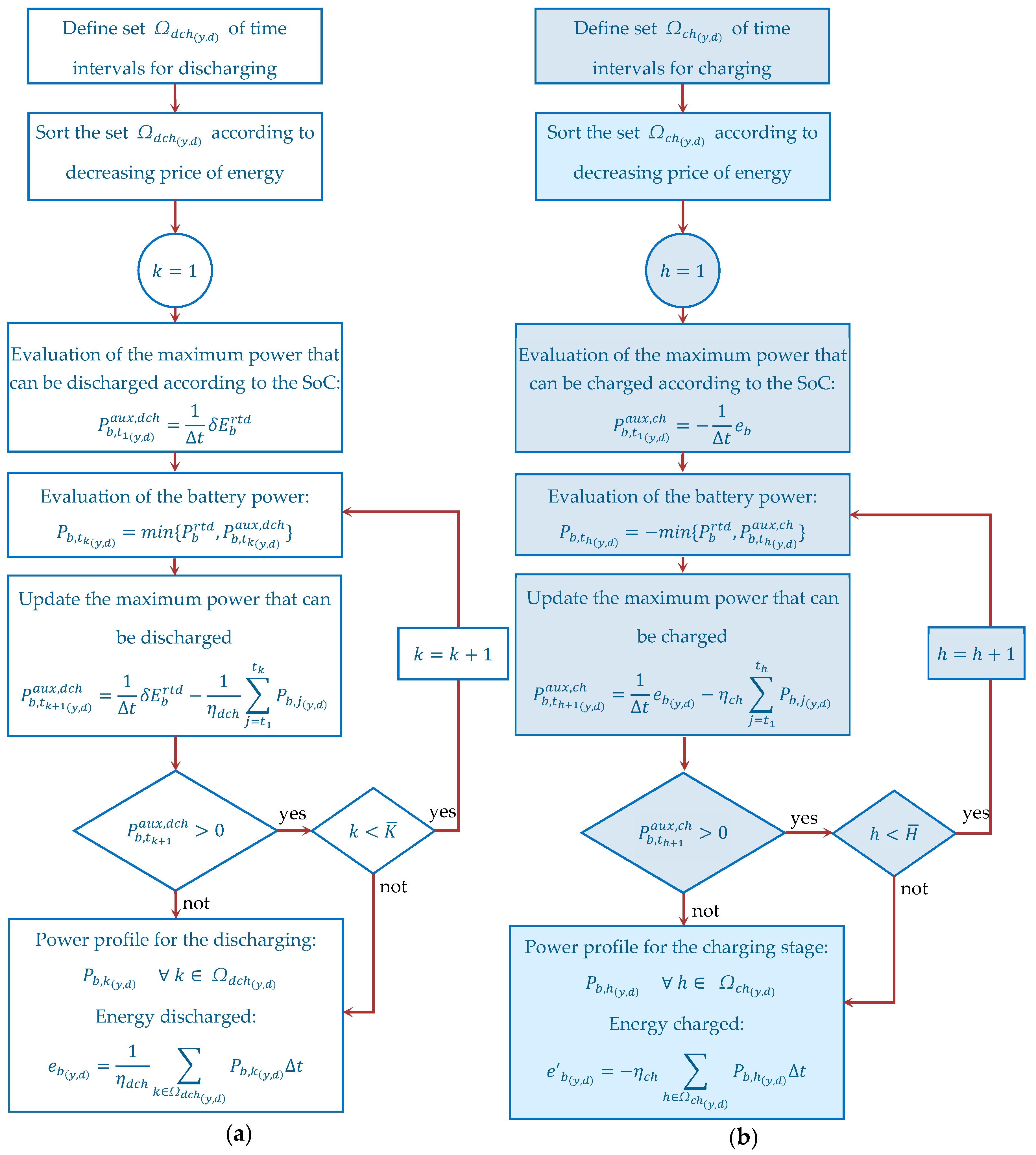
4.3. Operation Cost
- -
- sustained by the µG’s owner to (i) supply the loads, (ii) charge the EESSs, (iii) compensate for the power losses;
- -
- avoided thanks to the EESS discharged energy.
4.4. Cost of Voltage Dips
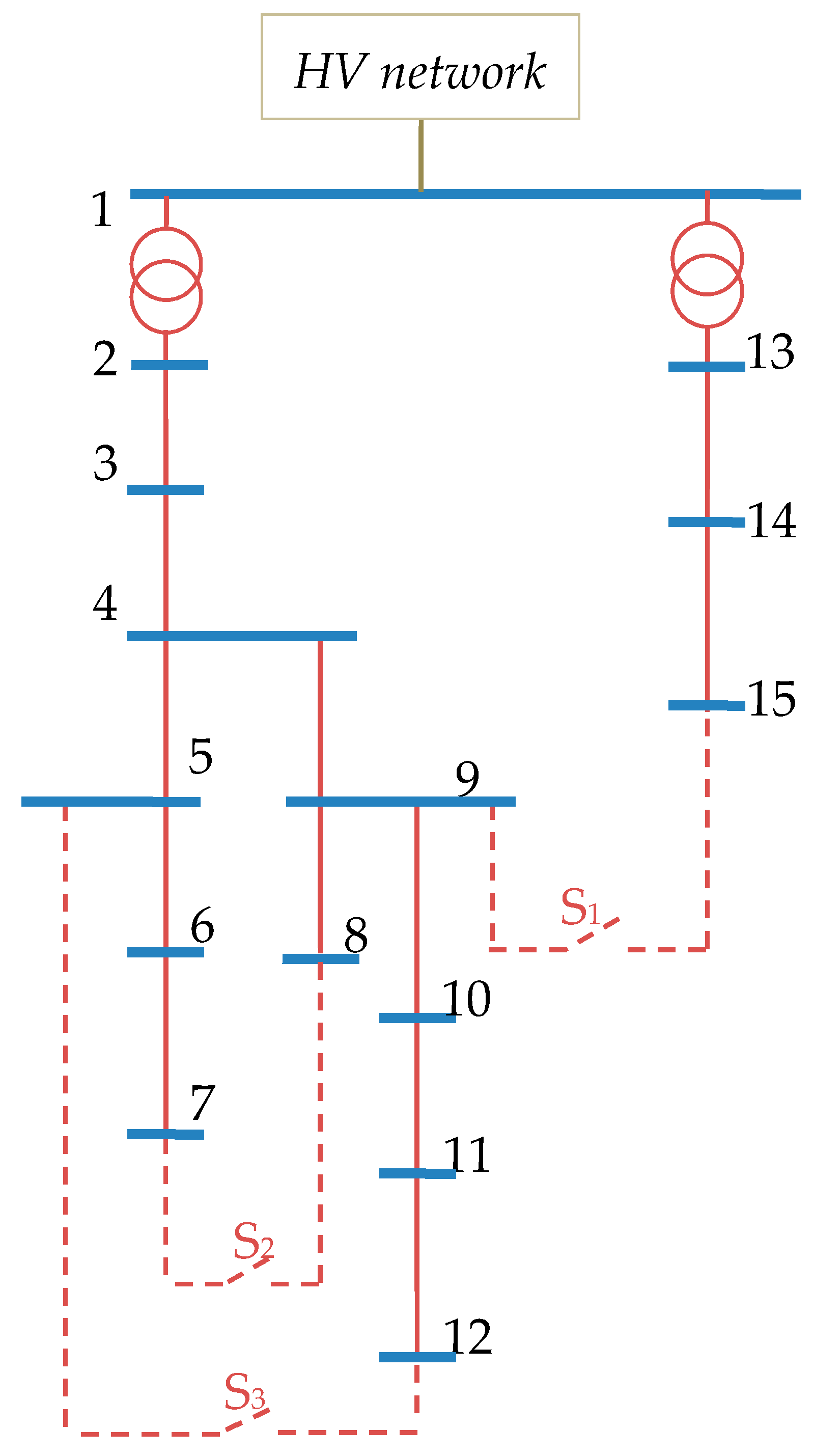
5. Numerical Applications
- -
- Case 1: S1, S2, S3: open
- -
- Case 2: S1, S2, and S3: closed
- -
- Case 3: S1: closed, S2, S3: open
- -
- Case 4: S1, S3: open, S2: closed
- -
- Case 5: S1, S2: open, S3: closed
- -
- Case 6: Case 1 (0.45), Case 2 (0.10), Case 3 (0.15), Case 4 (0.15), Case 5 (0.15)
6. Conclusions
Author Contributions
Funding
Acknowledgments
Conflicts of Interest
References
- Ai Wong, L.; Ramachandaramurthy, V.K.; Taylor, P.; Ekanayake, J.B.; Walker, S.L.; Padmanaban, S. Review on the optimal placement, sizing and control of an energy storage system in the distribution network. J. Energy Storage 2019, 21, 489–504. [Google Scholar] [CrossRef]
- Hemmati, R.; Shafie-Khah, M.; Catalão, J.P.S. Three-Level Hybrid Energy Storage Planning Under Uncertainty. IEEE Trans. Ind. Electron. 2019, 66, 2174–2184. [Google Scholar] [CrossRef]
- Zhang, N.; Li, R.; Jiang, Y. Cost-benefits analysis of battery storage system for industry consumers based on different operation modes. In Proceedings of the 2018 IEEE 2nd International Electrical and Energy Conference (CIEEC), Beijing, China, 4–6 November 2018; pp. 527–531. [Google Scholar] [CrossRef]
- Saboori, H.; Hemmati, R.; Sadegh Ghiasi, S.M.; Dehghan, S. Energy storage planning in electric power distribution networks—A state-of-the-art review. Renew. Sustain. Energy Rev. 2017, 79, 1108–1121. [Google Scholar] [CrossRef]
- Carpinelli, G.; Celli, G.; Mocci, S.; Mottola, F.; Pilo, F.; Proto, D. Optimal Integration of Distributed Energy Storage Devices in Smart Grids. IEEE Trans. Smart Grid 2013, 4, 985–995. [Google Scholar] [CrossRef]
- Grover-Silva, E.; Girard, R.; Kariniotakis, G. Optimal sizing and placement of distribution grid connected battery systems through an SOCP optimal power flow algorithm. Appl. Energy 2018, 219, 385–393. [Google Scholar] [CrossRef]
- Carpinelli, G.; Mottola, F.; Proto, D. Probabilistic sizing of battery energy storage when time-of-use pricing is applied. Electr. Power Syst. Res. 2016, 141, 73–83. [Google Scholar] [CrossRef]
- Electricity Energy Storage Technology Options: A White Paper Primer on Applications Costs and Benefits. 2010. Available online: https://www.epri.com/ (accessed on 12 January 2020).
- Carpinelli, G.; Di Perna, C.; Caramia, P.; Varilone, P.; Verde, P. Methods for Assessing the Robustness of Electrical Power Systems Against Voltage Dips. IEEE Trans. Power Deliv. 2009, 24, 43–51. [Google Scholar] [CrossRef]
- Caramia, P.; Varilone, P.; Verde, P.; Vitale, L. Tools for Assessing the Robustness of Electrical System against Voltage Dips in terms of Amplitude, Duration and Frequency. In Proceedings of the International Conference on Renewable Energies and Power Quality (ICREPQ’14), Cordoba, Spain, 8–10 April 2014. [Google Scholar]
- Küfeoğlu, S.; Lehtonen, M. Macroeconomic Assessment of Voltage Sags. Sustainability 2016, 8, 1304. [Google Scholar] [CrossRef]
- Ding, Z.; Zhu, Y.; Chen, C. Economic loss assessment of voltage sags. In Proceedings of the CICED 2010 Proceedings, Nanjing, China, 13–16 September 2010; pp. 1–5. [Google Scholar]
- 6th CEER Benchmarking Report on the Quality of Electricity and Gas Supply; CEER, 2016. Available online: https://www.ceer.eu/1305/ (accessed on 12 January 2020).
- Nick, M.; Cherkaoui, R.; Paolone, M. Optimal siting and sizing of distributed energy storage systems via alternating direction method of multipliers. Int. J. Electr. Power Energy Syst. 2015, 72, 33–39. [Google Scholar] [CrossRef]
- Nojavan, S.; Majidi, M.; Esfetanaj, N.N. An efficient cost-reliability optimization model for optimal siting and sizing of energy storage system in a microgrid in the presence of responsible load management. Energy 2017, 139, 89–97. [Google Scholar] [CrossRef]
- Lin, Z.; Hu, Z.; Zhang, H.; Song, Y. Optimal ESS allocation in distribution network using accelerated generalised Benders decomposition. IET Gener. Transm. Distrib. 2019, 13, 2738–2746. [Google Scholar] [CrossRef]
- Fantauzzi, M.; Lauria, D.; Mottola, F.; Scalfati, A. Sizing energy storage systems in DC networks: A general methodology based upon power losses minimization. Appl. Energy 2017, 187, 862–872. [Google Scholar] [CrossRef]
- Nick, M.; Cherkaoui, R.; Paolone, M. Optimal Allocation of Dispersed Energy Storage Systems in Active Distribution Networks for Energy Balance and Grid Support. IEEE Trans. Power Syst. 2014, 29, 2300–2310. [Google Scholar] [CrossRef]
- Andreotti, A.; Carpinelli, G.; Mottola, F.; Proto, D.; Russo, A. Decision Theory Criteria for the Planning of Distributed Energy Storage Systems in the Presence of Uncertainties. IEEE Access 2018, 6, 62136–62151. [Google Scholar] [CrossRef]
- Celli, G.; Pilo, F.; Pisano, G.; Soma, G.G. Including voltage dips mitigation in cost-benefit analysis of storages. In Proceedings of the 2018 18th International Conference on Harmonics and Quality of Power (ICHQP), Ljubljana, Slovenia, 13–16 May 2018; pp. 1–6. [Google Scholar] [CrossRef]
- IEC 61000-4-11:2004. Testing and Measurement Techniques—Voltage Sags, Short Interruptions and Voltage Variations Immunity Tests. 2004. Available online: https://webstore.iec.ch (accessed on 12 January 2020).
- Carpinelli, G.; Caramia, P.; Di Perna, C.; Varilone, P.; Verde, P. Complete Matrix Formulation of Fault Position Method for Voltage Dip Characterization. IET Gener. Transm. Distrib. 2007, 1, 56–64. [Google Scholar] [CrossRef]
- IEEE Standard 1346. Recommended Practice for Evaluating Electric Power System Compatibility with Electronic Process Equipment; The Institute of Electrical and Electronics Engineers, Inc.: New York, NY, USA, 1998. [Google Scholar]
- Xu, B.; Oudalov, A.; Ulbig, A.; Andersson, G.; Kirschen, D.S. Modeling of Lithium-Ion Battery Degradation for Cell Life Assessment. Trans. Smart Grid 2018, 9, 1131–1140. [Google Scholar] [CrossRef]
- Han, X.; Lu, L.; Zheng, Y.; Feng, X.; Li, Z.; Li, J.; Ouyang, M. A review on the key issues of the lithium ion battery degradation among the whole life cycle. ETransportation 2019, 1, 100005. [Google Scholar] [CrossRef]
- Fumagalli, E.; Lo Schiavo, L.; Delestre, F. Service Quality Regulation in Electricity Distribution and Retail; Springer: Berlin/Heidelberg, Germany, 2007. [Google Scholar]
- Di Fazio, A.R.; Duraccio, V.; Varilone, P.; Verde, P. Voltage sags in the automotive industry: Analysis and solutions. Electr. Power Syst. Res. 2014, 110, 25–30. [Google Scholar] [CrossRef]
- Weldemariam, L.; Cuk, V.; Cobben, J. Cost Estimation of Voltage Dips in Small Industries Based on Equipment Sensitivity Analysis. Smart Grid Renew. Energy 2016, 7, 271–292. [Google Scholar] [CrossRef]
- Bertazzi, A.; Fumagalli, E.; Lo Schiavo, L. The use of customer outage cost surveys in policy decision-making: The Italian experience in regulating quality of electricity supply. In Proceedings of the CIRED 2005—18th International Conference and Exhibition on Electricity Distribution, Turin, Italy, 6–9 June 2005; pp. 1–5. [Google Scholar]
- Delibera n. 155/02, Testo Integrato delle Disposizioni Dell’autorità per L’energia Elettrica e il Gas in Materia di Continuità del Servizio di Distribuzione Dell’energia Elettrica, G.U. Serie Generale n. 201 del 28 Agosto 2002. Available online: https://www.arera.it/it/docs/02/155-02.htm (accessed on 12 January 2020). (In Italian).
- Bollen, M.; Beyer, Y.; Styvactakis, E.; Trhulj, J.; Vailati, R.; Friedl, W. A European Benchmarking of voltage quality regulation. In Proceedings of the 2012 IEEE 15th International Conference on Harmonics and Quality of Power, Hong Kong, China, 17–20 June 2012; pp. 45–52. [Google Scholar]
- Delfanti, M.; Fumagalli, E.; Garrone, P.; Grilli, L.; Lo Schiavo, L. Toward Voltage-Quality Regulation in Italy. IEEE Trans. Power Deliv. 2010, 25, 1124–1132. [Google Scholar] [CrossRef]
- Weldemariam, L.E.; Cuk, V.; Cobben, J.F.G. A proposal on voltage dip regulation for the Dutch MV distribution networks. Int. Trans Electr. Energy Syst. 2019, 29, e2734. [Google Scholar] [CrossRef]
- Relazione Annuale Sullo Stato dei Servizi e Sull’ Attività Svolta. AEEGSI Annual Report AEEGSI. 2018. Available online: www.autorita.energia.it (accessed on 12 January 2020). (In Italian).
- Benchmark Systems for Network Integration of Renewable and Distributed Energy Resources, Cigré Task Force C6.04, Cigré Brochure 575. 2014. Available online: https://e-cigre.org/ (accessed on 12 January 2020).
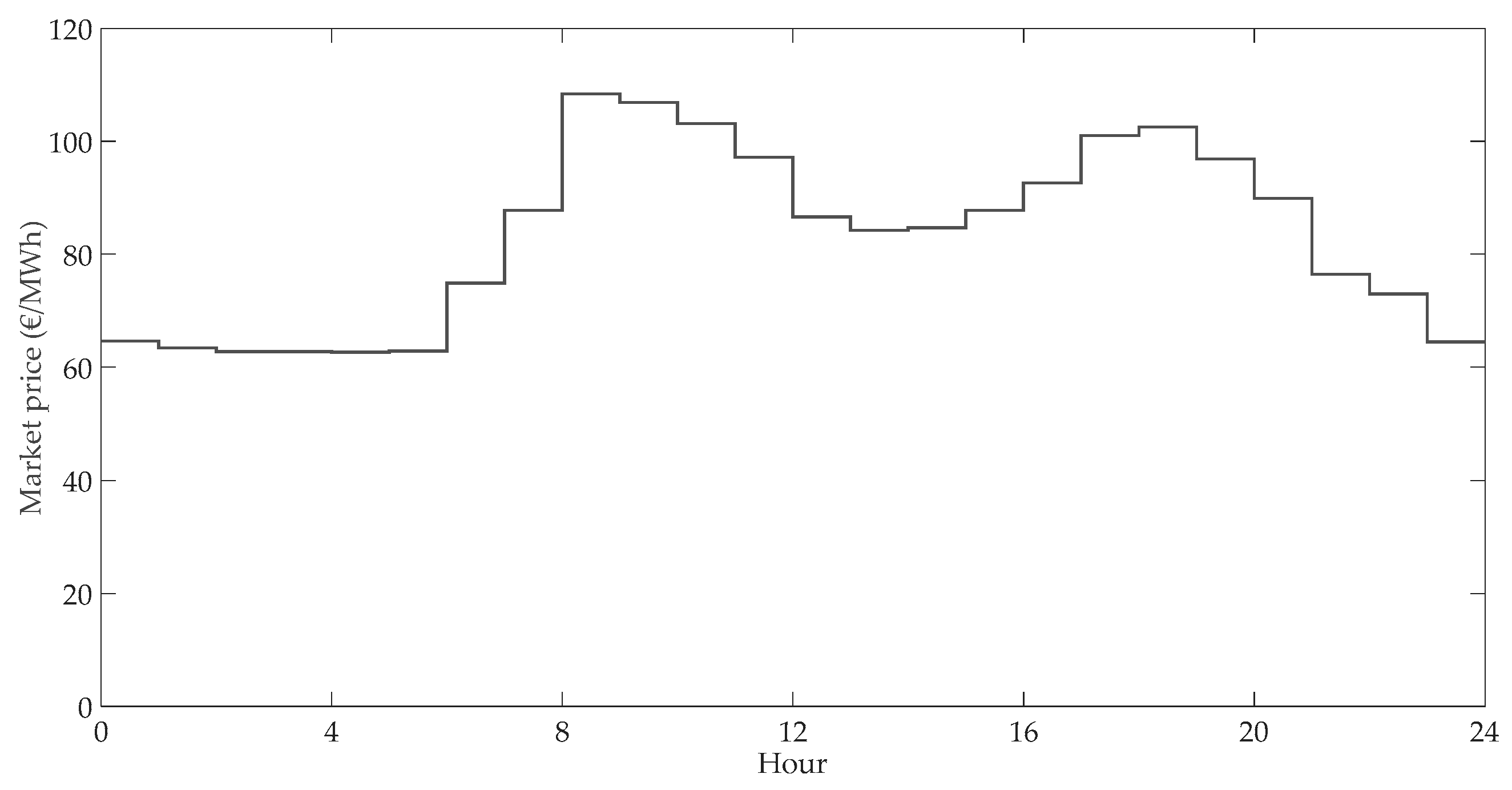
- Gestore Mercati Energetici. Esiti Mercato Elettrico, November 2019. Available online: https://www.mercatoelettrico.org/it/ (accessed on 12 January 2020).
- IRENA. Electricity Storage and Renewables: Costs and Markets to 2030, International Renewable Energy Agency, Abu Dhabi. 2017. Available online: http://www.irena.org/publications/2017/Oct/Electricity-storage-and-renewables-costs-and-markets (accessed on 12 January 2020).


| Residual Voltage [%] | Annual Average Voltage Dip Number | ||||
|---|---|---|---|---|---|
| Duration of the Voltage Dips [ms] | |||||
| 20–200 | 200–500 | 0.5–1 × 10³ | 1–5 × 10³ | 5–60 × 103 | |
| 80 ≤ u ≤ 90 | 33.93 | 4.35 | 0.93 | 0.34 | 0.05 |
| 70 ≤ u ≤ 80 | 12.91 | 3.01 | 0.38 | 0.21 | 0.07 |
| 40 ≤ u ≤ 70 | 17.07 | 3.95 | 0.31 | 0.11 | 0.03 |
| 5 ≤ u ≤ 40 | 5.22 | 1.39 | 0.12 | 0.02 | 0.00 |
| 1 ≤ u ≤ 5 | 0.27 | 0.05 | 0.07 | 0.03 | 0.10 |
| Total | 69.4 | 12.74 | 1.82 | 0.72 | 0.25 |
| Bus # | Rated Power (MVA) | Load Type | cos φ | Bus # | Rated Power (MVA) | Load Type | cos φ |
|---|---|---|---|---|---|---|---|
| 2 | 13.8 | Residential | 0.93 | 8 | 0.30 | Comm./industrial | 0.95 |
| 9.16 | Comm./industrial | 0.87 | 9 | 0.25 | Residential | 0.90 | |
| 3 | 0.35 | Residential | 0.95 | 0.20 | Comm./industrial | 0.90 | |
| 0.80 | Comm./industrial | 0.85 | 10 | 0.35 | Residential | 0.95 | |
| 4 | 0.25 | Residential | 0.90 | 11 | 0.50 | Residential | 0.90 |
| 0.24 | Comm./industrial | 0.80 | 12 | 0.10 | Residential | 0.95 | |
| 5 | 0.40 | Residential | 0.90 | 0.45 | Comm./industrial | 0.85 | |
| 6 | 0.20 | Residential | 0.95 | 13 | 3.20 | Residential | 0.90 |
| 0.30 | Comm./industrial | 0.85 | 3.78 | Comm./industrial | 0.87 | ||
| 7 | 0.15 | Residential | 0.95 | 14 | 0.68 | Comm./industrial | 0.85 |
| 8 | 0.10 | Residential | 0.95 | 15 | 0.27 | Comm./industrial | 0.90 |
| Parameter | Value | Parameter | Value |
|---|---|---|---|
| Battery round trip efficiency | 99 % | Battery Cycle life | 4800 cycles |
| Maximum Depth of Discharge | 100 % | Converter round trip efficiency | 98 % |
| Battery installation cost | 153 $/kWh | Converter installation cost | 59.6 $/kW |
| Battery replacement cost | 110 $/kWh | Maintenance cost | 1.5% |
| Case Study | |||||
|---|---|---|---|---|---|
| Case 1 | Case 2 | Case 3 | Case 4 | Case 5 | Case 6 |
| 3 | 6 | 8 | 3 | 3 | 8 |
| 4 | 7 | 9 | 4 | 4 | 9 |
| 5 | 8 | 10 | 5 | 5 | 10 |
| 6 | 9 | 11 | 6 | 6 | 11 |
| Case Study | Accounting for Voltage Dip Costs | BF (M$) | Voltage Dip Cost Reduction (M$) | EESSs’ Nodes | EESSs’ Sizes (MW) | ||
|---|---|---|---|---|---|---|---|
| EESS n. 1 | EESS n. 2 | EESS n. 1 | EESS n. 2 | ||||
| 1 | Yes | 4.81 | 1.63 | 3 | 6 | 10 | 10 |
| No | 3.19 | - | 3 | 6 | 10 | 10 | |
| 2 | Yes | −0.16 | 0.44 | 6 | - | 5 | - |
| No | −0.59 | - | 9 | - | 5 | - | |
| 3 | Yes | −0.34 | 0.31 | 9 | - | 5 | - |
| No | −0.65 | - | 9 | - | 5 | - | |
| 4 | Yes | 4.75 | 1.63 | 3 | 6 | 10 | 10 |
| No | 3.16 | - | 3 | 4 | 15 | 5 | |
| 5 | Yes | 4.70 | 1.63 | 3 | 6 | 10 | 10 |
| No | 3.21 | - | 3 | 5 | 5 | 15 | |
| 6 | Yes | 4.46 | 0.50 | 8 | 10 | 15 | 10 |
| No | 3.96 | - | 8 | 10 | 15 | 10 | |
| Case Study | Percentage Value of the Voltage Dip Cost Reduction on the Total Benefit (%) | Percentage of Value of the Voltage Dip Cost Reduction on the Installation and Replacement Cost (%) |
|---|---|---|
| 1 | 33.89 | 6.55 |
| 4 | 34.32 | 6.55 |
| 5 | 34.68 | 6.55 |
| 6 | 11.21 | 1.61 |
© 2020 by the authors. Licensee MDPI, Basel, Switzerland. This article is an open access article distributed under the terms and conditions of the Creative Commons Attribution (CC BY) license (http://creativecommons.org/licenses/by/4.0/).
Share and Cite
Mottola, F.; Proto, D.; Varilone, P.; Verde, P. Planning of Distributed Energy Storage Systems in μGrids Accounting for Voltage Dips. Energies 2020, 13, 401. https://doi.org/10.3390/en13020401
Mottola F, Proto D, Varilone P, Verde P. Planning of Distributed Energy Storage Systems in μGrids Accounting for Voltage Dips. Energies. 2020; 13(2):401. https://doi.org/10.3390/en13020401
Chicago/Turabian StyleMottola, Fabio, Daniela Proto, Pietro Varilone, and Paola Verde. 2020. "Planning of Distributed Energy Storage Systems in μGrids Accounting for Voltage Dips" Energies 13, no. 2: 401. https://doi.org/10.3390/en13020401
APA StyleMottola, F., Proto, D., Varilone, P., & Verde, P. (2020). Planning of Distributed Energy Storage Systems in μGrids Accounting for Voltage Dips. Energies, 13(2), 401. https://doi.org/10.3390/en13020401