Article

Fast Adaptive Robust Differentiator Based Robust-Adaptive Control of Grid-Tied Inverters with a New L Filter Design Method

1
Department of Electrical and Electronics Engineering, Sakarya University, Faculty of Engineering, 54050 Serdivan/Sakarya, Turkey
2
Research Group in Electrical Technologies for Sustainable and Renewable Energy (PAIDI-TEP-023), University of Cadiz, Higher Polytechnic School of Algeciras, 11202 Algeciras (Cadiz), Spain
3
Department of Electrical and Electronics Engineering, Sakarya University of Applied Sciences, 54050 Serdivan/Sakarya, Turkey
4
Department of Mechatronics Engineering, Faculty of Engineering, Balıkesir University, 10145 Balikesir, Turkey
5
Department of Energy Technology, Aalborg University, 9220 Aalborg, Denmark
*
Authors to whom correspondence should be addressed.
Energies 2020, 13(2), 360; https://doi.org/10.3390/en13020360
Submission received: 2 December 2019 / Revised: 7 January 2020 / Accepted: 8 January 2020 / Published: 11 January 2020
(This article belongs to the Section A2: Solar Energy and Photovoltaic Systems)

Abstract

:
In this research, a new nonlinear and adaptive state feedback controller with a fast-adaptive robust differentiator is presented for grid-tied inverters. All parameters and external disturbances are taken as uncertain in the design of the proposed controller without the disadvantages of singularity and over-parameterization. A robust differentiator based on the second order sliding mode is also developed with a fast-adaptive structure to be able to consider the time derivative of the virtual control input. Unlike the conventional backstepping, the proposed differentiator overcomes the problem of explosion of complexity. In the closed-loop control system, the three phase source currents and direct current (DC) bus voltage are assumed to be available for feedback. Using the Lyapunov stability theory, it is proven that the overall control system has the global asymptotic stability. In addition, a new simple L filter design method based on the total harmonic distortion approach is also proposed. Simulations and experimental results show that the proposed controller assurances drive the tracking errors to zero with better performance, and it is robust against all uncertainties. Moreover, the proposed L filter design method matches the total harmonic distortion (THD) aim in the design with the experimental result.

Graphical Abstract

1. Introduction

The significant proliferation of power electronics applications such as electrical drives, grid-coupled energy systems, residential applications, and induction systems further increases the existing concerns of the harmonics in power systems which have appeared due to the commonly used line side diode or thyristor rectifiers. This problem needs to be solved, because there are many international important standards which must be meet regarding the harmonics injected into the grid [1,2]. Other drawbacks of diode or thyristor rectifiers are the lagging power factor and low frequency [3,4,5]. On the one hand, the problem of lagging power factor can be solved by using a reactive power compensation circuit. On the other hand, there is hardly a possible way of implementing a high-performance industrial power electronics control application with these rectifiers due to the restriction on the operation frequency. These drawbacks create an important barrier in high performance and energy-efficient control applications. The best solution for this is to use PWM rectifiers, i.e., grid-tied inverters (GTIs). Unlike front-end rectifiers, GTIs offer many advantages such as compensation of harmonics and reactive power at the point of common coupling, sinusoidal line currents at the power factor near to unity, higher robust performance in direct current (DC) bus voltage regulation, and the ability to operate in four quadrants [6,7].
In general, the main purposes of GTIs in a control is to regulate the DC bus voltage at a desired level and line currents at the unity power factor. The traditional approach to address this problem is to use a voltage-oriented control [6,8]. In classical (linear fixed gain) controllers, external disturbances in these two control (processes) loops affects each other. This leads to a low performance DC bus voltage control and similarly a low performance power factor control. Consequently, this means that the switching and conduction losses of the converter increase, and some reactive power appears in the grid side. These problems establish the motivation for this study, as well as many studies in the literature. Despite these superiorities, a GTI suffers from its complicated multi-input multi-output nonlinear characteristics and external disturbance uncertainties. In addition, one of the uncommon nonlinear dynamic that a GTI exhibits is its nonminimum phase property [9,10].
Hence, addressing the control problems of GTIs has been received with substantial attention of academics in recent times. Generally, fixed gain-based methods, i.e., proportional integral (PI) and proportional integral derivative (PID) controllers are highly adopted in most industrial power electronics applications due to their feasibility [11,12]. However, it is common that these controllers fail to provide high-performance conditions [13]. Numerous control methods based on linearization have been developed for the fast-dynamic response to load or line disturbances [9,10,14,15,16,17]. Though, it is important to note that these linearization methods cause cancellation of certain useful nonlinearity of the plant and need a priori knowledge of the plant [15]. For this purpose, many studies have been reported in the literature to focus on coping with nonlinear characteristics and uncertainties of GTIs.
Similarly, fuzzy [18,19] and passivity-based controls [20,21] require strong expert knowledge and an open-loop control scheme, respectively. The sliding-mode variable structure control [4,22,23,24] provides a trade-off between the chattering and the tracking precision. To model a variable structure controller, a two-time scale model using a PWM converter is applied to control the DC bus indirectly [25]. However, there is a requirement of a priori information about the plant. In [26], a sliding mode and PI controller were used to develop an internal current control loop and an external DC bus voltage control loop, respectively. Similarly, application was also found in [27]. Although it is obvious that a relatively high performance is achieved in the control of the DC bus voltage, it was indicated there that d-axis reference current is reliant on the externally required β parameter.
Furthermore, among the various adaptive control techniques, adaptive backstepping control is one of the most adopted method in uncertain systems, particularly those systems which do not meet the matching requirements [28,29,30,31]. Numerous applications of adaptive backstepping control are found in many research fields such as chaotic motion [32], adaptive synchronization [33], control of electrical drives [34,35,36,37,38,39,40], aircraft control [41,42], and power systems [43,44]. Similarly, a model-based reference adaptive control was developed in [45]. The problem of over-parameterization can be avoided but not the problem of singularity. In [46], a wind energy system was controlled via an exact model backstepping method. In the same way, a linearized-based adaptive backstepping controller with load resistance uncertainty was suggested in [47,48].
This paper provides a new nonlinear and adaptive state feedback controller and a new robust differentiator with a fast-adaptive law. There are two originalities of the proposed controller:
(I) The first originality lies in the fact that line resistance and inductance are considered uncertain in the design. In addition, all nonlinearities of GTIs are taken into account in the design and global asymptotic stability is achieved in the sense of Lyapunov stability theory. Moreover, the proposed controller does not have the disadvantages of open-loop DC bus voltage control, over-parametrization, and singularity.
(II) The second originality comes from the novel L filter design. This L filter (calculation) design method uses an analytical approach based on the Fourier expansion of the inverter output voltages. By means of the proposed L filter design method, it has been possible to meet the desired total harmonic distortion (THD) value at the inverter output currents.
The rest of this research work is organized as follows: The dynamics of GTIs are explained in Section 2. Section 3 covers the proposed controller and proposed robust differentiator with the classical L filter design procedure. In Section 4, the real-time realization of the proposed controller is provided. In addition, a comparison between the proposed control system and a PI based conventional control system is also presented in detail. Section 5 concludes the paper.

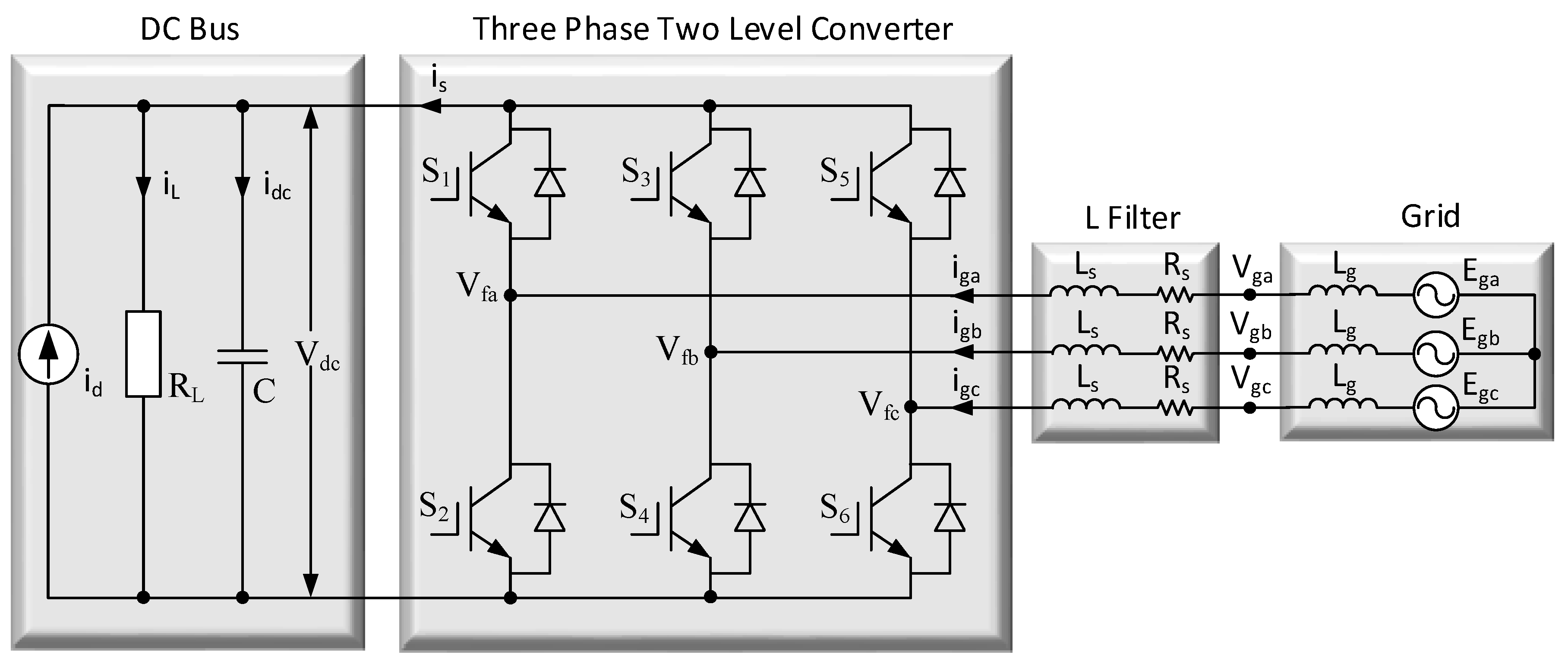
2. Dynamics of Grid-Tied Inverters

The most commonly used topology of GTI coupled to a three-phase balanced source is provided with an L filter in Figure 1. In Figure 1, Ls and Rs are the inductance and resistance components of the L filter, Cdc is the DC bus capacitor, Lg is the grid inductance, and il is the lumped external disturbance resulting from the total effect of iL and id. Empirically, the measurement and calculation of Cdc, Ls, and Rs are available, however, they fluctuate with time. As for the external load resistance, RL, it normally corresponds to an unknown variable resistance. Vdc also depicts the DC bus voltage.
Vga, Vgb, and Vgc are the three phase grid voltages, and iga, igb, and igc are the three phase grid currents. The output current of the inverter is is, the DC bus current is idc, and the load current is iL. The current source id as an external disturbance is put in the scheme to meet the converter losses of GTI. S1-6 corresponds to the power switches such as IGBT or MOSFET.
The relationship among the output currents of GTIs is given by considering Remark 1 as:
i s = i d c + i L i d
Here, both iL and id are external disturbances with unknown values. The DC bus current is written as follows:
i d c = C d c d V d c d t
Rearranging (1) is obtained:
i s = C d c d V d c d t + i L i d
The power equality between the DC side and AC side can be written in (4), provided Remark 2 is considered as:
V d c i s = 3 2 ( E g d i g d + E g q i g q )
where Egd and Egq stand for d- and q-axis voltages of grid and igd and igq stands for d- and q-axis currents of the grid.
Remark 1.
It should be noted that the grid and DC bus powers cannot be directly taken equal without considering the converter losses (switching and conduction losses of the converter). It is because the power drawn from the grid comprises the converter losses and DC bus power. Therefore, the power equality between grid (AC) side and DC side can be preserved, if the converter losses are added to the model from the DC side as an external disturbance. With this aim, a current source with unknown value should be considered in parallel with the DC bus to represent the converter losses in the model of (6)–(8).
Putting (3) into (4) undergoes the following equation:
V d c ( C d c d V d c d t + i L i d ) = 3 2 ( E g d i g d + E g q i g q )
Remark 2.
In balanced grid voltages, Egq equals zero under grid voltages synchronization using the phase locked loop (PLL) algorithm. In this work, synchronous reference frame PLL is used which ensure grid synchronization perfectly. Consequently, (5) can be changed as in (6). Then the d-q axis model of GTI can simply be arranged with the fact that Egd = Vgd and 0 = Egq ≅ Vgq, since Lg has a very low value (0.5151 mH here), [5,15,21,33,34,39,49] as:
d V d c d t = 3 V g d 2 C d c 1 V d c i g d 1 C d c i l
d i g d d t = R s L s i g d + ω s i g q + 1 L s ( V g d V c d )
d i g q d t = R s L s i g q ω s i g d 1 L s V c q
where Vcd and Vcq are the d- and q-axis input voltages of the inverter, and il is the lumped disturbance with the relationship that il = iL − id.

3. Control System Design for Grid-Tied Inverters

The main control objectives of the proposed controller, whose design methodology is developed based on the adaptive backstepping, are the following:
  • All the signals in the closed loop must be bounded and the tracking errors in the DC bus voltage/current globally asymptotically converge to zero under all uncertainties and;
  • To satisfy the unity power factor condition at the grid side;
  • Considering all the dynamics of GTIs, some common assumptions are used in the control objectives in the following order;
  • The three phase grid voltages Ega, Egb, and Egc are balanced. That is, the phase differences among the grid phase voltages are 120°, the peak values of them are 155 V, and the grid frequency is 50 Hz. Eventually the phase voltages are free of harmonic;
  • A three-phase transformer with a conversion ratio of 220/110 in the phase voltages is used as a grid. In this case, the secondary leakage inductance of the transformer constitutes the grid inductance for the control system, and its value is maximum (0.5151 mH) at the rated power, 5 kVA. For lower power values, its value is smaller than the maximum. Exactly like that, one can deduce the same result for the grid impedance;
  • The three-phase grid currents igabc and voltages Vgabc and DC bus voltage Vdc are present for feedback;
  • All external disturbances and the lumped disturbance iL, id, and il are bounded, and considered uncertain in the controller design;
  • Since the maximum value of Lg is very small as stated previously, Lg can be neglected. It is then valid that VgabcEgabc. It can be assumed from this case that the grid synchronization can be done correctly with a standard PLL algorithm [24,45];
  • In the adaptive control, it is an essential assumption that uncertainties are constants. The uncertainties with cap and with tilde represent values of estimations and estimation errors, respectively. Therefore, the time derivatives of uncertainties can be taken equal to zero, but not the derivatives of estimations and estimation errors [40];
    x ˜ = x x ^ , x ˜ ˙ = x ^ ˙ , x = ( R s , L s , C d c , i l )
  • The signal V d c r e f is the reference DC bus voltage signal, which is differentiable and bounded with derivatives.
    V d c r e f , V ˙ d c r e f L

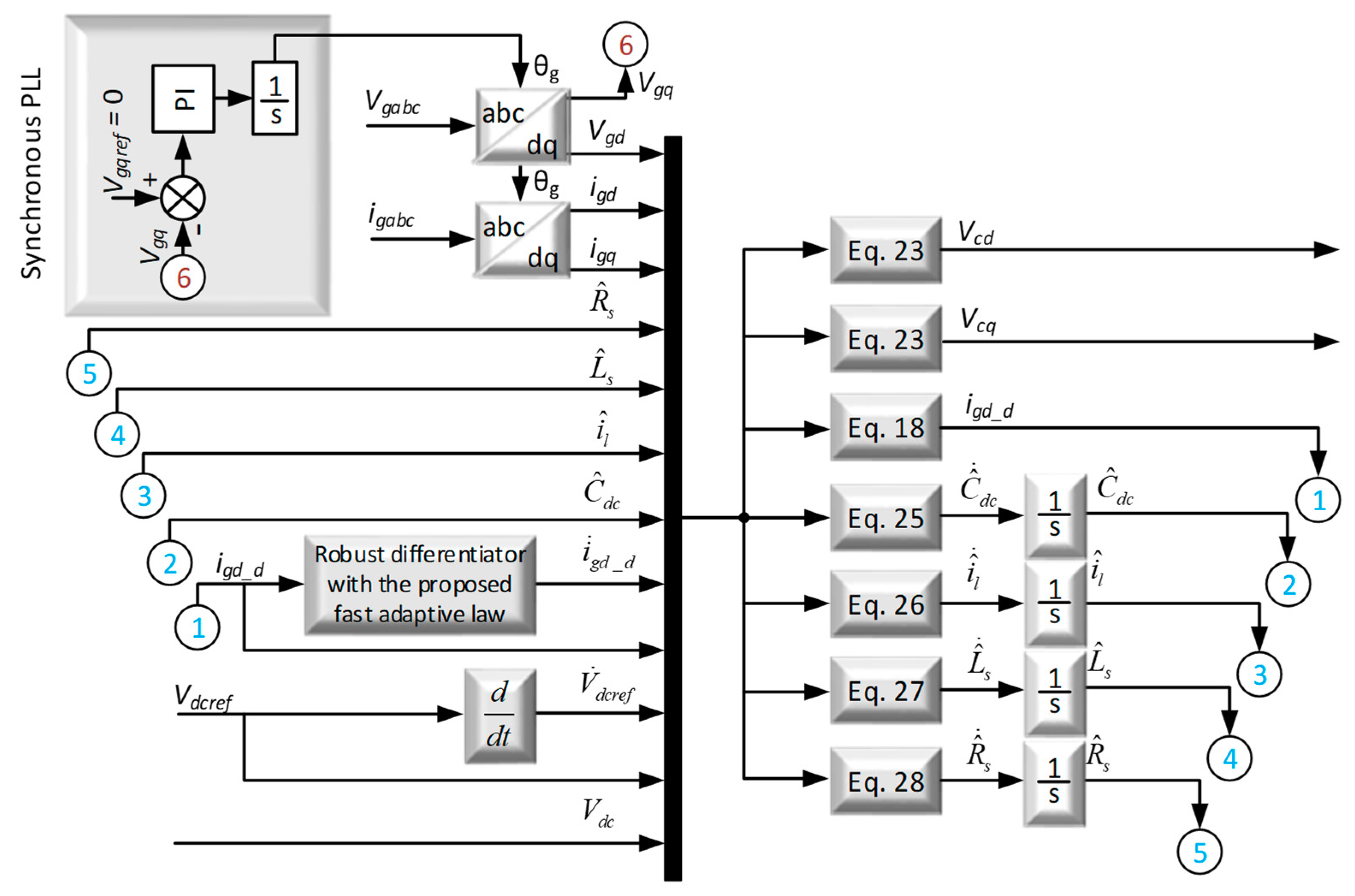
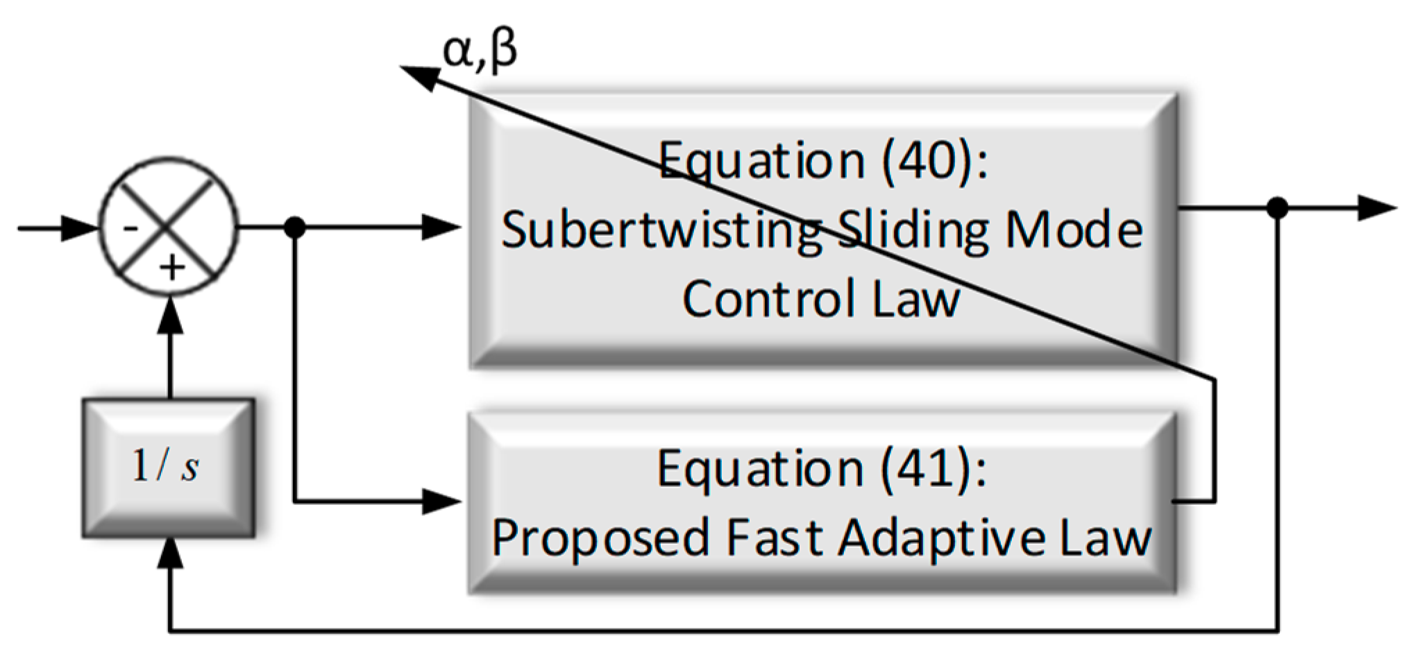
3.1. Proposed Controller Design

Using the above assumptions, the proposed controller can be designed using the backstepping technique. The following three steps are considered for this purpose:
Step 1 The tracking error dynamics in DC bus voltage is regulated by designing the d-axis reference current. The DC bus voltage tracking error can be written as:
e d c = V d c V d c r e f
where Vdcref is the reference DC bus voltage signal.
The first positive definite Lyapunov function to regulate the DC bus voltage tracking error dynamics can be defined as:
V 1 = C d c 2 V g d e d c 2 + 1 2 θ 1 C ˜ d c 2 + 1 2 θ 2 i ˜ l 2
where θ1 and θ2 are positive finite adaptation gains.
Taking the time derivative of (12) it gives:
V ˙ 1 = C d c V g d e d c ( 3 V g d 2 C d c 1 V d c i g d 1 C d c i l V ˙ d c r e f ) + 1 θ 1 C ˜ d c C ˜ ˙ d c + 1 θ 2 i ˜ l i ˜ ˙ l
Its latest form is formed with adaptations as:
V ˙ 1 = e d c ( 3 2 i g d V d c ( i ^ l + i ˜ l ) V g d V ˙ d c r e f ( C ^ d c + C ˜ d c ) V g d ) 1 θ 1 C ˜ d c C ^ ˙ d c 1 θ 2 i ˜ l i ^ ˙ l
The d- and q-axis current tracking errors can be written as:
e g d = i g d i g d _ d
e g q = i g q i g q _ d
where igq_d is the q-axis reference current, which is used to ensure the unity power factor, and the d-axis reference current (in other words, the virtual control input) is represented by igd_d.
Using (15), (14) becomes:
V ˙ 1 = e d c ( 3 2 ( e g d + i g d _ d ) V d c ( i ^ l + i ˜ l ) V g d V ˙ d c r e f ( C ^ d c + C ˜ d c ) V g d ) 1 θ 1 C ˜ d c C ^ ˙ d c 1 θ 2 i ˜ l i ^ ˙ l
Then, the DC bus voltage tracking error dynamics is completed to be regulated at this point by designing the d-axis reference current as a virtual control input.
i g d _ d = ( 2 V d c 3 ) ( i ^ l V g d + V ˙ d c r e f C ^ d c V g d k 1 e d c )
where k1 indicates the feedback gain.
Using (18) into (17), it is found the time derivative of the Lyapunov function.
V ˙ 1 = k 1 e d c 2 + 3 e d c e g d 2 V d c e d c i ˜ l V g d e d c V ˙ d c r e f C ˜ d c V g d 1 θ 1 C ˜ d c C ^ ˙ d c 1 θ 2 i ˜ l i ^ ˙ l
An indefinite term 3edcegd/2Vdc appears in (19), called the cross-term. This term is to be eliminated out by designing the d-axis input voltage, Vcd, to stabilize the d-axis current-tracking error dynamics.
Step 2 Next, the d- and q-axis current tracking error dynamics are stabilized by designing the d- and q-axis input voltages of GTI. First, the second Lyapunov function for the d- and q-axis current-tracking error dynamics is inserted via (15) and (16) as follows:
V 2 = 1 2 L s e g d 2 + 1 2 L s e g q 2 + 1 2 θ 3 L ˜ s 2 + 1 2 θ 4 R ˜ s 2
where θ3 and θ4 are adaptation gains.
Its time derivative becomes:
V ˙ 2 = e g d [ i g d R s + ω s i g q L s + V g d V c d i ˙ g d d L s ] + e g q [ i g q R s ω s i g d L s V c q ] 1 θ 3 L ˜ s L ^ ˙ s 1 θ 4 R ˜ s R ^ ˙ s
With adaptations, (21) gives:
V ˙ 2 = e g d [ i g d ( R ^ s + R ˜ s ) + ω s i g q ( L ^ s + L ˜ s ) + V g d V c d i ˙ g d d ( L ^ s + L ˜ s ) ] 1 θ 3 L ˜ s L ^ ˙ s 1 θ 4 R ˜ s R ^ ˙ s + e g q [ i g q ( R ^ s + R ˜ s ) ω s i g d ( L ^ s + L ˜ s ) V c q ]
Consequently, the d- and q-axis input voltages of the inverter are inserted as:
V c d = 3 e d c 2 V d c i ˙ g d d L ^ s i g d R ^ s + ω s i g q L ^ s + V g d + k 2 e g d V c q = i g q R ^ s ω s i g d L ^ s + k 3 e g q
where k2 and k3 stand for positive constant feedback gains.
The sum of both, V = V1 + V2, consisting of the DC bus and current-tracking errors provides the final Lyapunov function given by:
V ˙ = k 1 e d c 2 k 1 e g d 2 k 1 e g q 2 C ˜ d c ( 1 θ 1 C ^ ˙ d c + e d c V ˙ d c r e f V g d ) i ˜ l ( 1 θ 2 i ^ ˙ l + e d c V g d ) L ˜ s ( 1 θ 3 L ^ ˙ s + e g d i ˙ g d d e g d ω s i g q + e g q ω s i g d ) R ˜ s ( 1 θ 4 R ^ ˙ s + e g d i g d + e g q i g q )
Step 3 Here, the parameter adaptation laws are achieved, and thus the global asymptotic stability is guaranteed for the closed-loop system. For this purpose, the time derivative of the final Lyapunov function in (24) is negative semidefinite if the parameter update laws are taken in the form of:
C ^ ˙ d c = θ 1 ( e d c V ˙ d c r e f V g d )
i ^ ˙ l = θ 2 ( e d c V g d )
L ^ ˙ s = θ 3 ( e g d i ˙ g d d + e g d ω s i g q e g q ω s i g d )
R ^ ˙ s = θ 4 ( e g d i g d e g q i g q )
Substituting (25)–(28) into (24), it yields:
V ˙ = k 1 e c 2 k 2 e d s 2 k 3 e q s 2
Which means that there is a non-positive or a negative semidefinite time derivative of the final Lyapunov function, outside the equilibrium point (0,0,0) in the (edc,egd,egq) coordinates.
Remark 3.
There is no way of designing adaptive and feedback gains in an analytical way. Hence, their values can be found using trial-and-error approach. This process is called the final adjustment [18].
Proposition 1.
The resultant closed-loop control system is globally asymptotically stable.
Proof. 
Using standard signal-chasing algorithms, it is clear that 0     V ( )     V ( 0 )   <   and V ( )     L from (40). So, ( e dc , e gd , e gq ,   R ˜ s ,   L ˜ s ,   C ˜ dc ,   i ˜ d ,   i ˜ L )     L . From the control objective vi, (   R ^ s ,   L ^ s ,   C ^ dc ,   i ^ d ,   i ^ L )     L . From the control objective vii, ( V dcref , V dc , i gd _ d , i gd , i gq )     L . From the conclusions above, (   e ˙ dc ,   e ˙ gd ,   e ˙ gq ,   V ˙ dc ,   i ˙ gd ,   i ˙ gq ,   i ˙ gd _ d , V cd , V cq )     L . ( e dc , e gd , e gq ) are uniformly continuous signals since ( e ˙ dc ,   e ˙ gd ,   e ˙ gq )     L . In addition, ( e dc , e gd , e gq )     L 2 . Using Barbalat’s Lemma with the conclusions of ( e ˙ dc ,   e ˙ gd ,   e ˙ gq )     L and ( e dc , e gd , e gq )     L 2 , it is clear that ( e dc , e gd , e gq )     ( 0 , 0 , 0 ) as t     0 . With positive finite feedback and adaptation gains, all the signals in the closed-loop system remain bounded and all tracking errors asymptotically converge to zero, whatever the initial conditions, which means that the closed-loop control system is globally asymptotically stable. □
Remark 4.
In such control systems, parameter estimations converge to real values if the persistence of excitation condition (the control input reference is sufficiently rich in frequency to satisfy persistence of excitation) can be met. In GTI control systems, a constant DC bus voltage reference is generally applied to the control system; and therefore, the condition is not met. As a consequence, all the estimations converge to some constants (not real values) where control inputs ( V c d , V c q , i g d _ d ) asymptotically drive tracking errors ( e g d , e g q , e d c ) to zero.

3.2. Proposed L Filter Design

For the L filter design, a recent method is given in (30) [16]. In this technique, the harmonic component is over the switching frequency, Vh%, is about 0.45 for modulation index (m) values of the sinusoidal PWM close to 1.0 [16].
L V h % V g a r m s 2 ω n m f P 1 T H D i
where mf is the frequency modulation.
The selection criteria of Vh% strongly depends on modulation index [16]. This study presents best results among the L filter design methods in the literature. To obtain a clearer and more systematic way to design the L filter for GTIs, a total harmonic distortion (THD) approach-based design method is proposed below. For the power system given in Table 1, the L filter can be designed selecting the THD of phase currents (THDi) as 3.2%. With this value as the aim, the THDs of phase currents are expected to not exceed 3.2% in experiments. The L filter is designed for the power system whose parameters are given in Table 1.
Firstly, the modulation index is defined as:
m = V n 2 0.612 V d c = 110 2 0.612 350 = 0.8895
(31) means that 3850 W active power is transferred into grid at m = 0.8895 for 350 V DC bus voltage. The voltage harmonics of sinusoidal PWM around switching frequency, up to 4 mf, are expressed for m = 0.8895, as:
m f 2 = 0.0947 V d c , 2 m f 1 = 0.0902 V d c , 3 m f 2 = 0.0442 V d c , 3 m f 4 = 0.0474 V d c , 4 m f 1 = 0.0383 V d c , 4 m f 5 = 0.0381 V d c , 4 m f 7 = 0.0127 V d c
For a finite analysis, the harmonics up to 4 mf are only considered in the design. For 3850 W active power to be transferred into grid, the rms value of the grid phase currents and the rms value of their THD, respectively, are expressed as follows:
I p h a s e _ r m s = P 3 p h a s e 3 V l i n e = 3850 ( 3 190 ) = 11.6989 A I p h a s e _ r m s _ T H D = I p h a s e _ r m s T H D = 11.7 0.032 = 0.3744 A
In this case, the THD equality can be written as:
I p h a s e _ r m s _ T H D = 2 ( 0.0947 V d c x L ) 2 + 2 ( 0.0902 V d c 2 x L ) 2 + 2 ( 0.0474 V d c 3 x L + 0.0442 V d c 3 x L ) 2 + 2 ( 0.0383 V d c 4 x L + 0.0381 V d c 4 x L + 0.0128 V d c 4 x L ) 2
where XL is the inductive reactance of the L filter around switching frequency.
For the side band harmonics around mf, 2 mf, 3 mf, and 4 mf, the individual inductive reactance is taken equal to XL, 2 XL, 3 XL, and 4 XL, respectively, that is, the frequency difference among the side band harmonics is neglected since it does not have an effect on the result. Consequently, it is calculated as:
x L = 0.4244 V d c = 147.82 Ω
From the XL above, the L filter is thus designed below.
L = x L 2 π f s w = 147.82 2 π 10000 = 0.002352 H
This design can easily be extended to space vector PWM by rewriting harmonics around switching frequency.

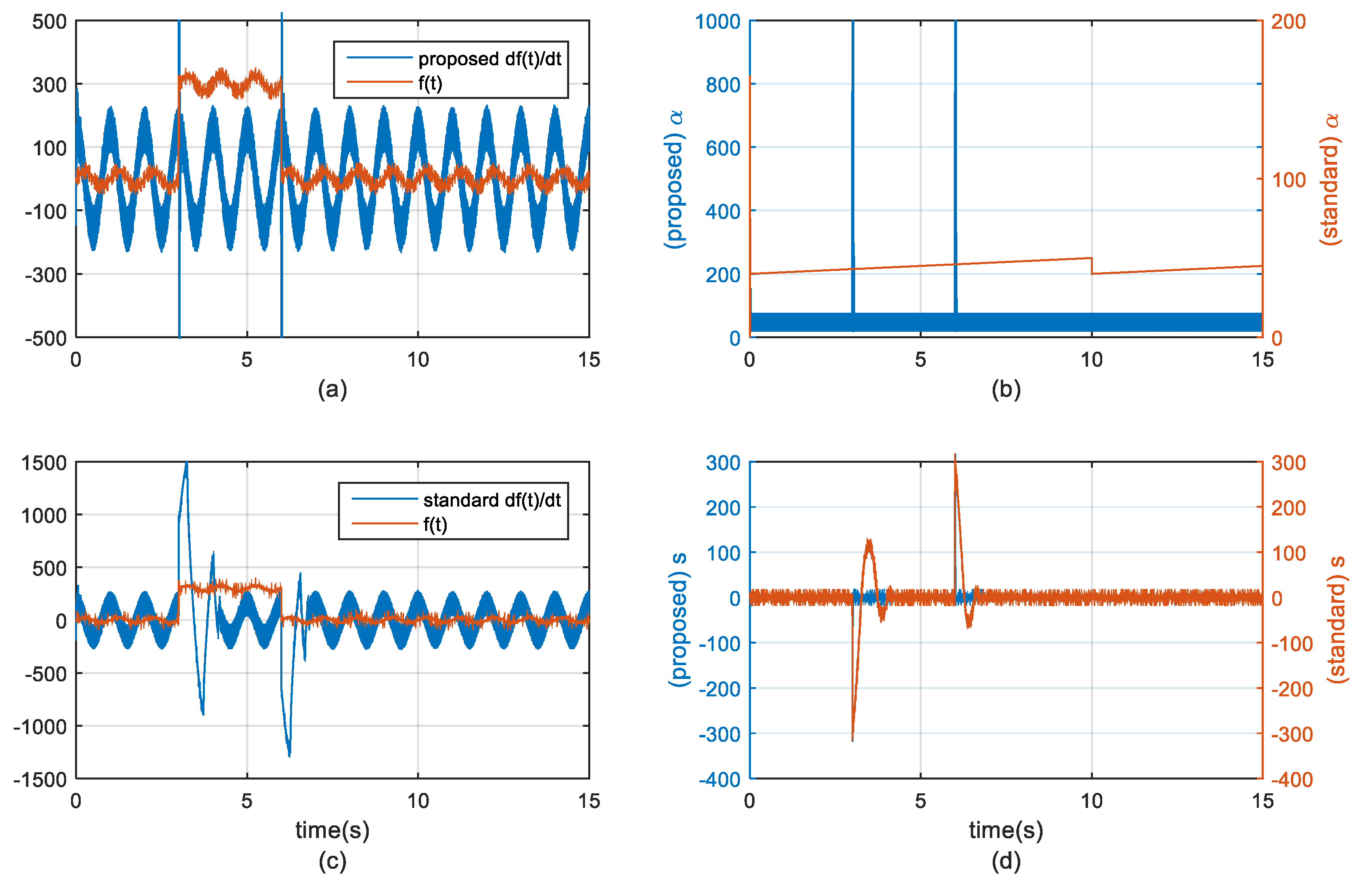
3.3. Proposed Robust Differentiator Design

In this part, a robust differentiator is developed to calculate the time derivative of the virtual control input since the numerical derivative of such noisy signals can be problematic in control systems. Using Lipschitz’s constant C > 0 an auxiliary function is then defined to differentiate the input signal as:
x ˙ = u
The sliding surface can be written as:
s = x i g d _ d ( t )
Differentiating s provides the following:
s ˙ = u i ˙ g d _ d ( t )
The super-twisting control law below can be, thus, defined in [49,50,51].
The theorem-type environments can be formatted as follows:
u = i ˙ g d _ d = α | s | 1 2 s i g n ( s ) + v v ˙ = β 2 s i g n ( s )
where the adaptive gains are defined as:
α ˙ = { ω 1 γ 1 2 s i g n ( | s | μ ) + k | s | | s | + υ   i f ( α > α m ) η i f ( α α m ) β = 2 ε α
where ε , γ 1 , ω 1 , η , α m , μ , k , υ are arbitrary constants.
Proposition 2.
Given that α ( 0 ) > α m and α ( 0 ) > μ , there is a finite time t F > 0 via the differentiator of (40) with the adaptive gains (41). Thus, the sliding variable s goes the limit of | s | < μ in a finite time t F .
Proof. 
The stability analysis of adaptive gain equations is carried out by Lyapunov function using linear matrix inequalities (LMI). In quadratic form, the Lyapunov function is written as:
V ( x ) = ζ T P ζ + 1 2 γ 1 ( α α * ) 2 + 1 2 γ 1 ( β β * ) 2 ζ T = [ ζ 1 ζ 2 ] = [ | s | 1 / 2 s i g n ( s ) s i g n ( s ) ]
α * and β * are some positive constants, and P is positive definite matrix as:
P = P T > 0
The solution of Lyapunov equations depends on the selection of a special A matrix, which stems from the Hurwitz characteristic polynomial as:
p ( s ) = s 2 + 1 2 α s + 1 2 β
A T P + P A < 0
A = [ 1 2 α 1 2 β 0 ]
The inequality ( x 2 + y 2 + z 2 ) | x | + | y | + | z | is based on derivative of (42). e α = α α * and e β = β β * can be written. Then, it follows as V ˙ ( t ) | s | 1 2 ζ T Q ζ 1 γ 1 e α α ˙ 1 γ 2 e β β ˙ V ˙ ( t ) | s | 1 2 ζ T Q ζ ω 1 2 γ 1 | e α | ω 2 2 γ 2 | e β | . By selecting e α , β = ω 2 ω 1 γ 2 γ 1 , α and β is obtained in (41) [51]. According to the Lyapunov direct method, the derivative of Lyapunov function is obtained in (47):
V ˙ ( t ) | s | 1 2 ζ T Q ζ 1 γ 1 ( α α * ) α ˙ 1 2 γ 1 ( β β * ) β ˙
where Q, P, and A are symmetric and positive definite matrixes, thus, the LMI-based Lyapunov equations satisfy sufficient stability conditions. □
Proposition 3.
The adaptive gains stay bounded in the adaptive second order sliding mode, and their values are decreasing in the limit | s | < μ .
Proof. 
Outside the limit | s | < μ , a solution to (41) can be given as the following function (increasing) in (48):
α ( t ) = α ( 0 ) + ( ω 1 γ 1 2 + k | s | | s | + υ ) t , 0 t t F
Inside the limit | s | < μ , a solution to (41) can be recreated as the following function (decreasing) in (49):
α ( t ) = α ( 0 ) + ( ω 1 γ 1 2 + k | s | | s | + υ ) t , ω 1 γ 1 2 > k | s | | s | + υ
Consequently, α ( t ) and β ( t ) are bounded signals and they are decreasing functions inside the limit | s | < μ . As the sliding mode surface error approaches zero, the quadratic term will take very little value. So, conventional adaptation law persists robustness based on possible minimum gain. υ in the term k | s | | s | + υ makes the numerator smaller than denominator, which results in quadratic term close to zero. For more details, please refer to [47]. □
A new fast-adaptive law given in (41) constitutes the second originality of the study, and it was developed based on the adaptive law proposed in [51]. The proposed differentiator possesses three important superiorities as follows:
  • The controller design can be carried out with ease, by avoiding the complexity in the existing backstepping;
  • It can differentiate fast varying signals without the chattering;
  • It enables differentiation of noisy signals to be possible without amplifying the noise;
  • There is no need for using a filter, for example notch filter commonly preferred in DC bus voltage control loop [52].
The block scheme of the proposed differentiator is given in Figure 2 and an example simulation is provided in Figure 3.
Remark 5.
The standard adaptive law is given in (50) as proposed in [51]:
α ˙ = { ω 1 γ 1 2 s i g n ( | s | μ ) i f α > α m η i f α α m   β = 2 ε α
The differentiator in (40) with the proposed adaptive law in (41) reaches the steady-state response faster than that with the standard adaptive law. To see the effectiveness of the proposed differentiator, the differentiation of a noisy signal is simulated by standard and proposed differentiators as demonstrated below:
Simulation (example as a case study) A noisy signal, f ( t ) = 25 sin ( 2 π t ) + n o i s e ± 300 , is used in this example as actual input signal of the differentiators and differentiations with the standard and proposed differentiators are presented below. The noise is generated by Gaussian stochastic processes, with the amplitude of about ±1. The gains of differentiators are chosen as:
μ = 1.5 , α ( 0 ) = 200 , α m = 50 , ω 1 = 500000 , γ 1 = 2 , ε = 100 , η = 1 , υ = 10 6 , k = 90000
equally for both differentiators.
As observed from Figure 3b, the adaptive gain, α, goes to αm for both them. As seen in Figure 3a,c, the chattering amplitudes, thus, remain at about the same level for two cases after the convergence. However, it is obvious that the proposed adaptive law enhances the convergence speed of the error dynamics. Figure 3d shows that the sliding surface keeps the noise out of the differentiation process. Consequently, the proposed differentiator manages to take the time derivative of a noisy signal with a fast convergence, without amplifying noise.
The ω and γ 1 / 2 are constant values in conventional adaptation law. Even if their numbers have large values, integration is carried out linearly. In the case of rapid changes in control such as abrupt reference changes, the conventional adaptation law does not react fast enough. In the conventional adaptation law, large ω and γ 1 / 2 values can increase the dynamical performance. Therefore, in the case of large values of sliding surface, large control effort can be obtained to drive the sliding surface to zero. Nevertheless, those large ω and γ 1 / 2 values cause a high chattering in the steady state for the zero-going sliding surface values.
As shown in Figure 3, it is evident that the proposed robust differentiator is superior to the conventional one in terms of smoothness, robustness, and fastness. The controller also has the ability of filtering the harmonic distortions in DC bus voltage. In the literature, in order to filter 2k (even order) harmonics in DC bus voltage, various kinds of second order (for example notch) filters are commonly used in DC bus voltage control loop in addition to the voltage controller [52]. Here, without using any kind of second-order filter, the proposed controller with the proposed fast-adaptive differentiator can achieve a better control performance.

3.4. Design of PLL

The PLL scheme with proposed controller is illustrated is Figure 4, and its transfer function is given for the three phase systems as:
G c l ( s ) = k p s + k i s 2 + k p s + k i
where kp and ki are the gains of the PI controller in the PLL scheme.
The PI gains are calculated for the damping ratio ξ = 1.0 as:
k i = f n 2 = 2500 k p = 2 ξ f n = 100

3.5. Design of Conventional PI Based Control System

To deduce the dq0 components from the abc signals, the d–q transformation is used in the following form:
[ U d U q U 0 ] = 2 3 [ cos ( θ ) cos ( θ 2 π 3 ) cos ( θ + 2 π 3 ) sin ( θ ) sin ( θ 2 π 3 ) sin ( θ + 2 π 3 ) 2 2 2 2 2 2 ] [ U a U b U c ]
For a comparison of the proposed controller versus classical PI-based controller, the following optimal procedure is used to design the PI controller gains [53]:
k d c = 2 V d c C d c 3 a d c T i n V g d T d c = a d c 2 T i n     ( a d c = 3 T i n = 4 T s ) k d q = L T / ( 2 T s ) T d q = a 2 T s a = 3
where Ts is the sampling time.
With these values, it is not possible to obtain a high-performance dynamical response without a final adjustment [18,53]. Therefore, with the gain of sinusoidal PWM (maximum duty cycle is 7500 of the DSP for 10 kHz), and after the final adjustment, the gains of the DC bus voltage PI controller are found as kp = 0.512 and ki = 5.21. The gains of the d- and q-axis current PI controllers are also calculated as kp = 112.8 and ki = 2053.4.

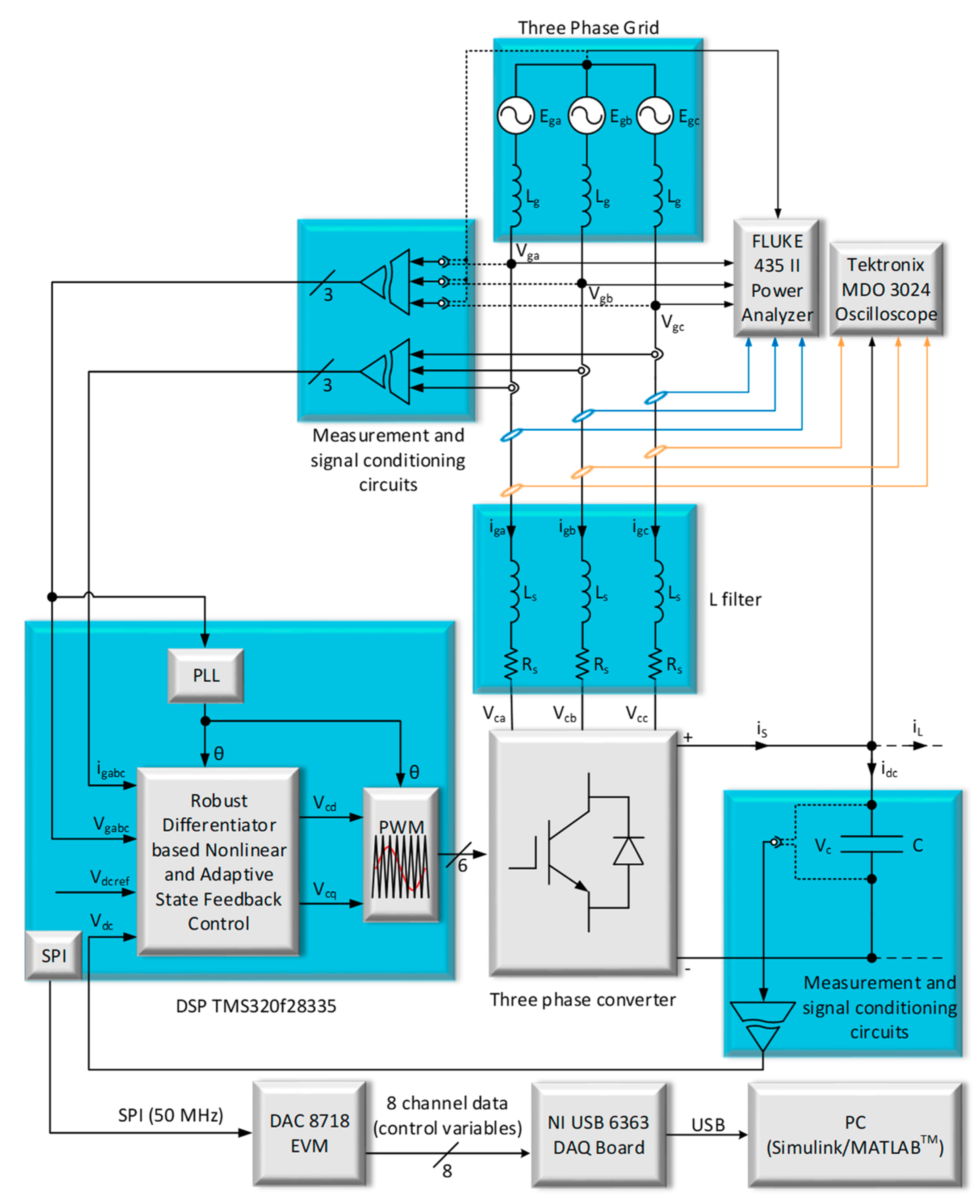
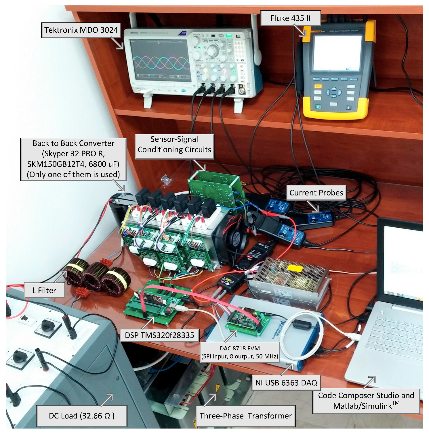
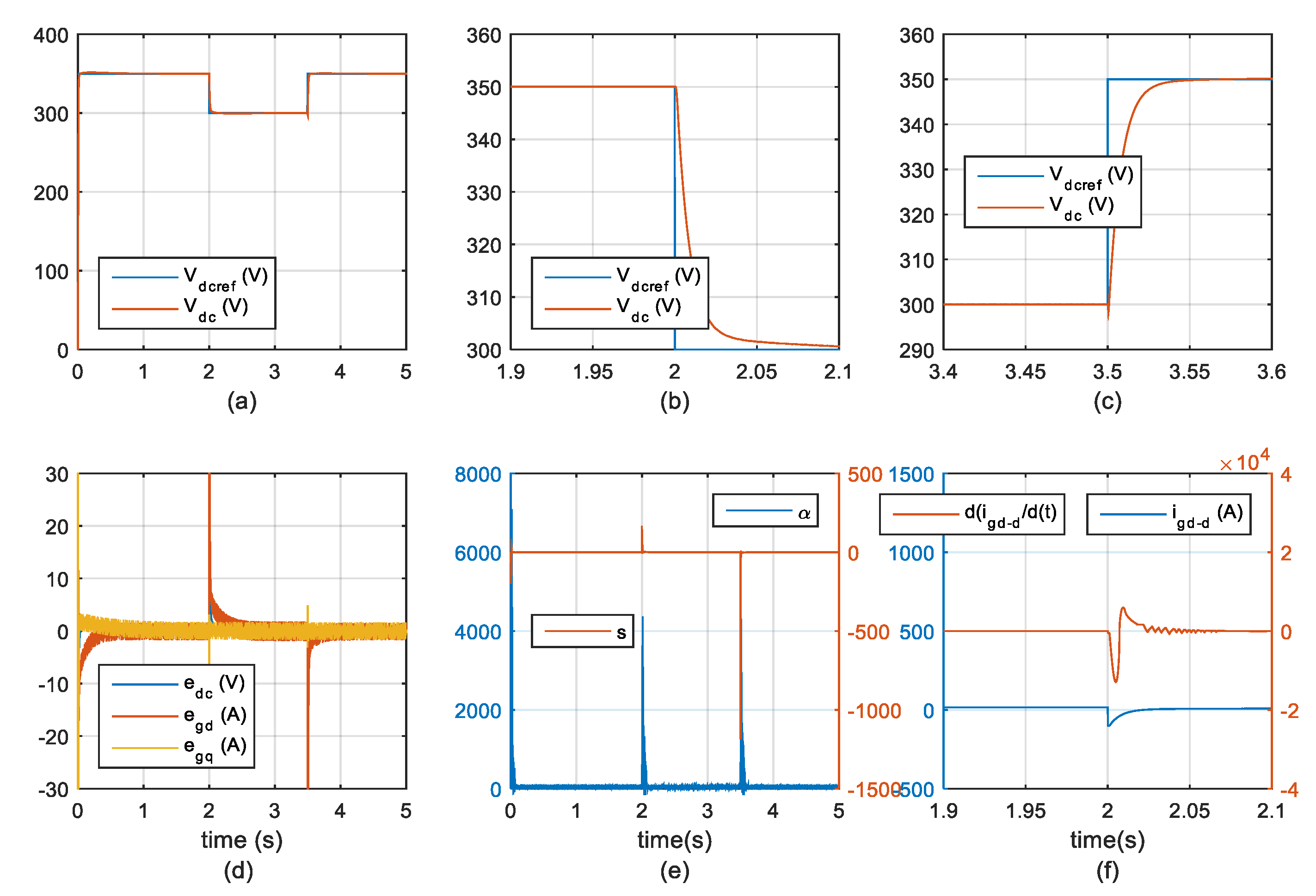
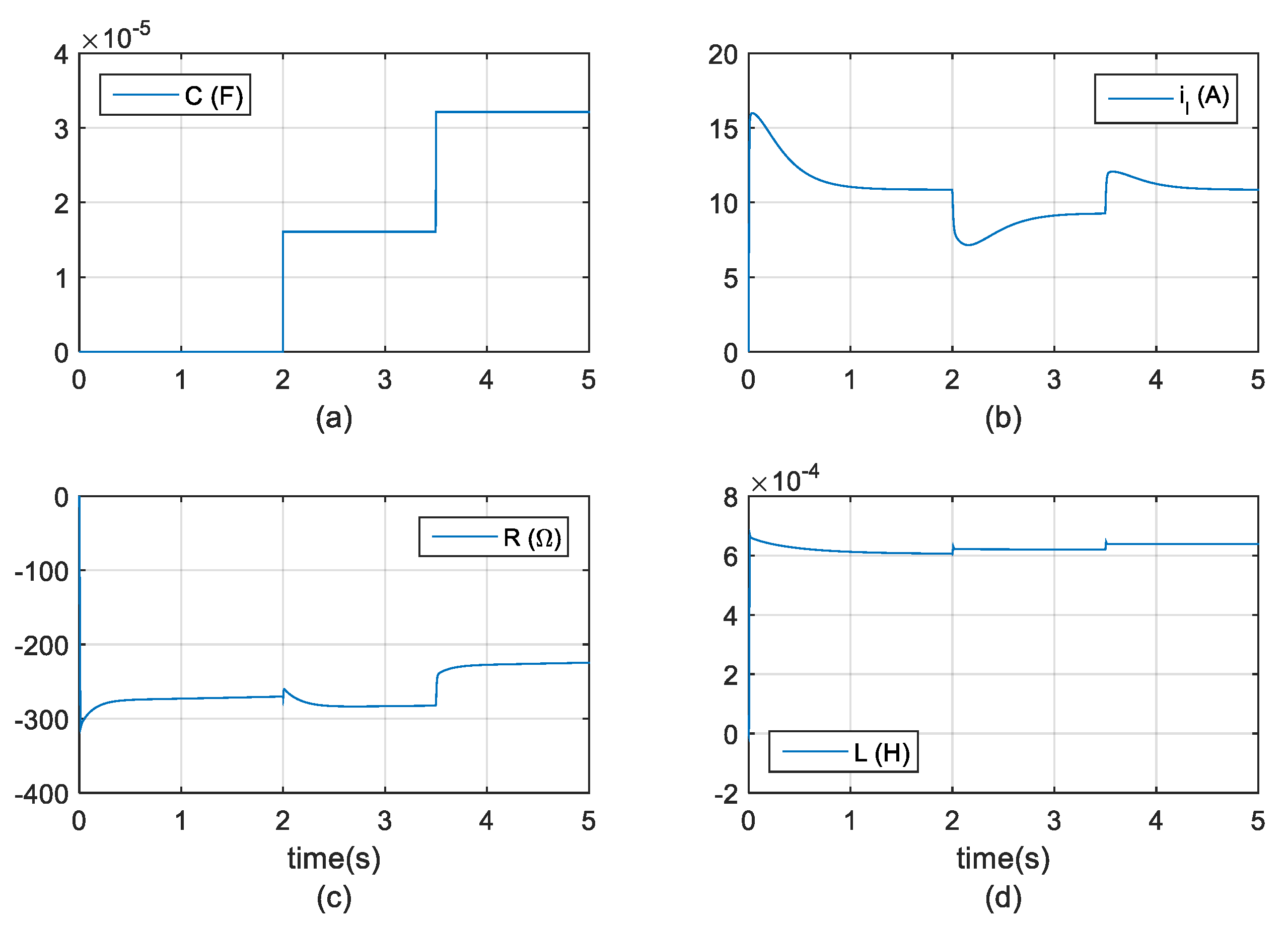
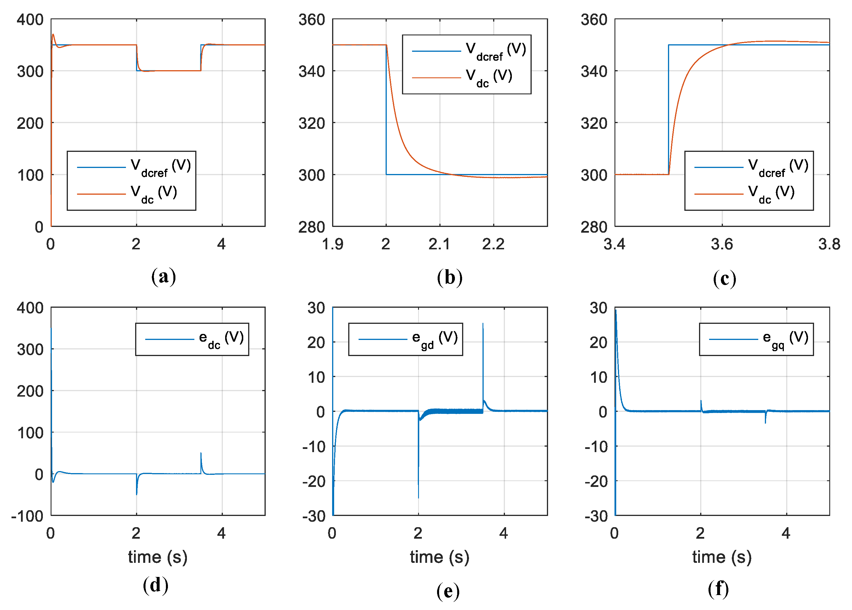
4. Experimental Results

Figure 5 illustrates the overall control scheme of GTI. A photo of experimental arrangement is given in Figure 6. In this work, the sampling and PWM frequencies are 10 kHz. All control operations (transformations, integrations, etc.) are coupled with the PWM frequency. The gains are k 1 = 0.01 , k 2 = 200 , k 3 = 200 , θ 1 = 10 8 , θ 2 = 1000 , θ 3 = 10 8 , θ 4 = 2 and all initial conditions are made to zero. As is the usual case [54,55], the control gains have been set by trial and error.
Similarly, in Figure 7, the error dynamics of the proposed system are provided. It is seen therein that the tracking errors remain stable around zero, that is, the DC bus voltage tracks the reference despite the uncertainties. The proposed differentiator drives the sliding surface to zero in a fast way without the chattering, since α converges to a very low value restricted by αm. In consequence, the differentiation of igd_d is accomplished without amplifying noise.
The parameter estimations of the DC bus capacitor estimation, external disturbance estimation, estimation of L filter resistance, and estimation of L filter inductance are shown in Figure 8. It is observed that all parameter and disturbance estimations remain bounded and converge to some constants where the tracking errors go to zero, as explained in Remark 4. As the control input reference (Vdcref) is a fixed value, persistence of excitation is not ensured, and the parameter estimates converge to some fixed (not true) values the way the state converge to the desired value asymptotically. For that reason, the estimated values are different from the true values [54,55].
In Figure 9, the results of the PI controller-based GTI system are given. It is clear from Figure 9 that Vdc tracks Vdcref with a low dynamic response as compared with the proposed controller. The proposed controller drives the DC bus voltage to the reference in 50 ms, whereas the PI controller takes 100 ms to drive the DC bus voltage to the reference. As a result, the same situation is also valid for egd and egq.
For further comparisons, three phase currents and THD in the grid phase current with the proposed controller and the PI controller are presented in Figure 10 and Figure 11, respectively.
The THD of the phase currents was 3.3% with the proposed method whereas it is 3.2% with the PI controller. The THD with the proposed controller is slightly higher than the THD with the PI controller, since the proposed controller has faster current control loops as observed in Figure 7 and Figure 9.

5. Conclusions

This paper presented a new nonlinear and adaptive state feedback controller with a new fast-adaptive robust differentiator for GTIs. No parameter knowledge was used in the modeling of the proposed controller and no external disturbance was available for feedback in the resulting closed-loop system. The robust differentiator was used with the proposed fast-adaptive structure to differentiate the reference q-axis current (virtual control input), without amplifying noise in the phase currents. The proposed differentiator also avoided the problem complexity in the existing backstepping.
The results showed that the THD of the phase currents with the PI controller was equal to the aimed value, 3.2%. However, the proposed controller possessed a faster dynamical performance than the PI controller, and thus the THD of the phase currents was slightly higher than the aimed value, 3.3%. It should be noted that the proposed controller excellently tracked a time-varying reference thanks to the faster dynamical behavior as compared with the PI control. Moreover, the proposed control scheme did not have the problems of singularity and over-parameterization. The proposed control system can also be easily extended to the GTI systems with LCL or LLCL filters. The experimental results proved the validity and feasibility of the proposed controller for GTI systems. A new simple L filter design method for GTIs was also proposed based on THD approach. Results verified that the proposed design closely met the aim of the THD in the phase currents.

Author Contributions

M.K., and T.K. designed the algorithm; M.K., and F.K. gathered the data and performed the experiment; F.B., and L.M.F.-R. evaluated the results and provided technical guidance at different stages. All authors have read and agreed to the published version of the manuscript.

Funding

This study is supported by the Scientific and Technological Research Council of Turkey (TUBITAK, project number: 114E159).

Acknowledgments

The authors thank the TUBITAK for giving the funding.

Conflicts of Interest

The authors declare no conflict of interest.

References

  1. Guo, X.Q.; Wu, W.Y.; Gu, H.R. Modeling and simulation of direct output current control for LCL-interfaced grid-connected inverters with parallel passive damping. Simul. Model. Pract. Theory 2010, 18, 946–956. [Google Scholar] [CrossRef]
  2. International Standard IEC 61000-3-2:2018 RLV|IEC Webstore|Electromagnetic Compatibility, International Electrotechnical Commission; International Standard IEC: Geneva, Switzerland, 2018.
  3. Bose, B.K. Modern Power Electronics and AC Drives, 1st ed.; Prentice Hall: Upper Saddle River, NJ, USA, 2002; ISBN 978-0130167439. [Google Scholar]
  4. Mohan, N.; Undeland, T.M.; Robbins, W.P. Power Electronics: Converters, Applications, and Design, 3rd ed.; Wiley Online Library: Hoboken, NJ, USA, 2002; ISBN 978-0-471-22693-2. [Google Scholar]
  5. Yacoubi, L.; Fnaiech, F.; Dessaint, L.A.; Al-Haddad, K. New nonlinear control of three-phase NPC boost rectifier operating under severe disturbances. In Proceedings of the Mathematics and Computers in Simulation, Vienna, Austria, 5–7 February 2003; Volume 63, pp. 307–320. [Google Scholar]
  6. Mao, H. Review of high-performance three-phase power-factor correction circuits. IEEE Trans. Ind. Electron. 1997, 44, 437–446. [Google Scholar]
  7. Cambronne, J.P.; Pierre, X. Synthesis of different synchronous modulators for high power three-phase/single-phase PWM converters. Math. Comput. Simul. 1998, 46, 413–423. [Google Scholar] [CrossRef]
  8. Kolar, J.W.; Friedli, T. The Essence of Three-Phase PFC Rectifier Systems—Part I—IEEE Journals Magazine. IEEE Trans. Power Electron. 2013, 28, 176–198. [Google Scholar] [CrossRef]
  9. Yin, B.; Oruganti, R.; Panda, S.K.; Bhat, A.K.S. A simple single-input-single-output (1. Yin, B.; Oruganti, R.; Panda, S.K.; Bhat, A.K.S. A simple single-input-single-output (SISO) model for a three-phase PWM rectifier. IEEE Trans. Power Electron. 2009, 24, 620–631. [Google Scholar] [CrossRef]
  10. Lee, T.S. Input-output linearization and zero-dynamics control of three-phase AC/DC voltage-source converters. IEEE Trans. Power Electron. 2003, 18, 11–22. [Google Scholar]
  11. Ang, K.H.; Chong, G.; Li, Y. PID control system analysis, design, and technology. IEEE Trans. Control Syst. Technol. 2005, 13, 559–576. [Google Scholar]
  12. Cichowlas, M.; Kamierkowski, M.P. Comparison of current control techniques for PWM rectifiers. In Proceedings of the IEEE International Symposium on Industrial Electronics, L’Aquila, Italy, 8–11 July 2002; Volume 4, pp. 1259–1263. [Google Scholar]
  13. Melício, R.; Mendes, V.M.F.; Catalão, J.P.S. Fractional-order control and simulation of wind energy systems with PMSG/full-power converter topology. Energy Convers. Manag. 2010, 51, 1250–1258. [Google Scholar] [CrossRef]
  14. Lee, D.C.; Lee, G.M.; Lee, K. Do DC-bus voltage control of three-phase ac/dc PWM converters using feedback linearization. IEEE Trans. Ind. Appl. 2000, 36, 826–833. [Google Scholar]
  15. Lee, T.-S. Nonlinear state feedback control design for three-phase PWM boost rectifiers using extended linearisation. IEE Proc. Electr. Power Appl. 2003, 150, 554. [Google Scholar] [CrossRef]
  16. León, A.E.; Solsona, J.A.; Busada, C.; Chiacchiarini, H.; Valla, M.I. High-performance control of a three-phase voltage-source converter including feedforward compensation of the estimated load current. Energy Convers. Manag. 2009, 50, 2000–2008. [Google Scholar] [CrossRef]
  17. Ye, Y.; Kazerani, M.; Quintana, V.H. Modeling, control and implementation of three-phase PWM converters. IEEE Trans. Power Electron. 2003, 18, 857–864. [Google Scholar]
  18. Bouafia, A.; Krim, F.; Gaubert, J.P. Design and implementation of high performance direct power control of three-phase PWM rectifier, via fuzzy and PI controller for output voltage regulation. Energy Convers. Manag. 2009, 50, 6–13. [Google Scholar] [CrossRef]
  19. Aissaoui, A.G.; Tahour, A.; Essounbouli, N.; Nollet, F.; Abid, M.; Chergui, M.I. A Fuzzy-PI control to extract an optimal power from wind turbine. Energy Convers. Manag. 2013, 65, 688–696. [Google Scholar] [CrossRef]
  20. Lee, T. Lagrangian Modeling and Passivity-Based Control of three-phase AC/DC voltage-source converters. IEEE Trans. Ind. Electron. 2004, 51, 892–902. [Google Scholar] [CrossRef]
  21. Gensior, A.; Sira-Ramirez, H.; Rudolph, J.; Guldner, H. On some nonlinear current controllers for three-phase boost rectifiers. IEEE Trans. Ind. Electron. 2009, 56, 360–370. [Google Scholar] [CrossRef]
  22. Liu, Y.; Li, X.Y. Decentralized robust adaptive control of nonlinear systems with unmodeled dynamics. IEEE Trans. Automat. Contr. 2002, 47, 848–856. [Google Scholar]
  23. Landau, I.D. From robust control to adaptive control. Control Eng. Pract. 1999, 7, 1113–1124. [Google Scholar] [CrossRef]
  24. Sugie, T.; Yoshikawa, T. Adaptive Robust Control of Robot Manipulators—Theory and Experiment. IEEE Trans. Robot. Autom. 1994, 10, 705–710. [Google Scholar]
  25. Vilathgamuwa, D.M.; Wall, S.R.; Jackson, R.D. Variable structure control of voltage sourced reversible rectifiers. IEEE Proc. Electr. Power Appl. 1996, 143, 18. [Google Scholar] [CrossRef]
  26. Naouar, M.W.; Ben Hania, B.; Slama-Belkhodja, I.; Monmasson, E.; Naassani, A.A. FPGA-based sliding mode direct control of single phase PWM boost rectifier. Math. Comput. Simul. 2013, 91, 249–261. [Google Scholar] [CrossRef]
  27. Fernando Silva, J. Sliding-mode control of boost-type unity-power-factor PWM rectifiers. IEEE Trans. Ind. Electron. 1999, 46, 594–603. [Google Scholar] [CrossRef]
  28. Krstić, M.; Kanellakopoulos, I.; Kokotović, P.V. Nonlinear and Adaptive Control Design; Wiley: New York, NY, USA, 1995; ISBN 9780471127321. [Google Scholar]
  29. Kokotović, P.V. The Joy of Feedback: Nonlinear and Adaptive. IEEE Control Syst. 1992, 12, 7–17. [Google Scholar]
  30. Zhang, T.; Ge, S.S.; Hang, C.C. Adaptive neural network control for strict-feedback nonlinear systems using backstepping design. Automatica 2000, 36, 1835–1846. [Google Scholar] [CrossRef]
  31. Yip, P.P.; Hedrick, J.K. Adaptive dynamic surface control: A simplified algorithm for adaptive backstepping control of nonlinear systems. Int. J. Control 1998, 71, 959–979. [Google Scholar] [CrossRef]
  32. Vincent, U.E.; Njah, A.N.; Laoye, J.A. Controlling chaos and deterministic directed transport in inertia ratchets using backstepping control. Physica D 2007, 231, 130–136. [Google Scholar] [CrossRef]
  33. Matouk, A.E.; Agiza, H.N. Bifurcations, chaos and synchronization in ADVP circuit with parallel resistor. J. Math. Anal. Appl. 2008, 341, 259–269. [Google Scholar] [CrossRef] [Green Version]
  34. Karabacak, M.; Eskikurt, H.I. Design, modelling and simulation of a new nonlinear and full adaptive backstepping speed tracking controller for uncertain PMSM. Appl. Math. Model. 2012, 36, 5199–5213. [Google Scholar] [CrossRef]
  35. El Magri, A.; Giri, F.; Abouloifa, A.; Chaoui, F.Z. Robust control of synchronous motor through AC/DC/AC converters. Control Eng. Pract. 2010, 18, 540–553. [Google Scholar] [CrossRef] [Green Version]
  36. Karabacak, M.; Eskikurt, H.I. Speed and current regulation of a permanent magnet synchronous motor via nonlinear and adaptive backstepping control. Math. Comput. Model. 2011, 53, 2015–2030. [Google Scholar] [CrossRef]
  37. Ting, C.S.; Chang, Y.N. Observer-based backstepping control of linear stepping motor. Control Eng. Pract. 2013, 21, 930–939. [Google Scholar] [CrossRef]
  38. Traoré, D.; De Leon, J.; Glumineau, A. Sensorless induction motor adaptive observer-backstepping controller: Experimental robustness tests on low frequencies benchmark. IET Control Theory Appl. 2010, 4, 1989–2002. [Google Scholar] [CrossRef]
  39. Trabelsi, R.; Khedher, A.; Mimouni, M.F.; M’Sahli, F. Backstepping control for an induction motor using an adaptive sliding rotor-flux observer. Electr. Power Syst. Res. 2012, 93, 1–15. [Google Scholar] [CrossRef]
  40. Xie, Q.; Han, Z.; Kang, H. Adaptive backstepping control for hybrid excitation synchronous machine with uncertain parameters. Expert Syst. Appl. 2010, 37, 7280–7284. [Google Scholar] [CrossRef]
  41. Mian, A.A.; Wang, D. Modeling and backstepping-based nonlinear control strategy for a 6 DOF quadrotor helicopter. Chin. J. Aeronaut. 2008, 21, 261–268. [Google Scholar] [CrossRef] [Green Version]
  42. Yang, J.H.; Hsu, W.C. Adaptive backstepping control for electrically driven unmanned helicopter. Control Eng. Pract. 2009, 17, 903–913. [Google Scholar] [CrossRef]
  43. Roy, T.K.; Mahmud, M.A.; Oo, A.M.T. Robust adaptive backstepping excitation controller design for higher-order models of synchronous generators in multimachine power systems. IEEE Trans. Power Syst. 2019, 34, 40–51. [Google Scholar] [CrossRef]
  44. Wang, K.; Xin, H.; Gan, D.; Ni, Y. Non-linear robust adaptive excitation controller design in power systems based on a new back-stepping method. IET Control Theory Appl. 2010, 4, 2947–2957. [Google Scholar] [CrossRef] [Green Version]
  45. Yacoubi, L.; Al-Haddad, K.; Dessaint, L.A.; Fnaiech, F. A DSP-based implementation of a nonlinear model reference adaptive control for a three-phase three-level NPC boost rectifier prototype. IEEE Trans. Power Electron. 2005, 20, 1084–1092. [Google Scholar] [CrossRef]
  46. El Magri, A.; Giri, F.; Elfadili, A.; Dugard, L. Wind sensorless control of wind energy conversion system with PMS generator. In Proceedings of the 2012 American Control Conference (ACC), Montreal, QC, Canada, 27–29 June 2012; pp. 2238–2243. [Google Scholar]
  47. Hadri-Hamida, A.; Allag, A.; Hammoudi, M.Y.; Mimoune, S.M.; Zerouali, S.; Ayad, M.Y.; Becherif, M.; Miliani, E.; Miraoui, A. A nonlinear adaptive backstepping approach applied to a three phase PWM AC-DC converter feeding induction heating. Commun. Nonlinear Sci. Numer. Simul. 2009, 14, 1515–1525. [Google Scholar] [CrossRef]
  48. Allag, A.; Hammoudi, M.Y.; Ayad, M.Y. Adaptive Backstepping Voltage Controller Design for an PWM AC-DC Converter. Int. J. Electr. Power Eng. 2007, 1, 62–69. [Google Scholar]
  49. Levant, A. Sliding order and sliding accuracy in sliding mode control. Int. J. Control 1993, 58, 1247–1263. [Google Scholar] [CrossRef]
  50. Levant, A. Robust Exact Differentiation via Sliding Mode Technique. Automatica 1998, 34, 379–384. [Google Scholar] [CrossRef]
  51. Shtessel, Y.; Taleb, M.; Plestan, F. A novel adaptive-gain supertwisting sliding mode controller: Methodology and application. Automatica 2012, 48, 759–769. [Google Scholar] [CrossRef]
  52. Kale, M.; Akar, F.; Karabacak, M. A SOGI Based Band Stop Filter Approach for a Single-Phase Shunt Active Power Filter. In Proceedings of the 2018 2nd International Symposium on Multidisciplinary Studies and Innovative Technologies (ISMSIT), Ankara, Turkey, 19–21 October 2018; pp. 1–4. [Google Scholar]
  53. Dannehl, J.; Wessels, C.; Fuchs, F.W. Limitations of voltage-oriented PI current control of grid-connected PWM rectifiers with LCL filters. IEEE Trans. Ind. Electron. 2009, 56, 380–388. [Google Scholar] [CrossRef]
  54. Kim, K.-S.; Kim, Y. Robust backstepping control for slew maneuver using nonlinear tracking function. IEEE Trans. Control Syst. Technol. 2003, 11, 822–829. [Google Scholar]
  55. Ioannou, P.A.; Sun, J. Robust Adaptive Control; Prentice Hall: Upper Saddle River, NJ, USA, 1995. [Google Scholar]
Figure 1. Basic topology of grid-tied inverters (GTIs).
Energies 13 00360 g001
Figure 2. Robust differentiator with the proposed fast adaptive law.
Energies 13 00360 g002
Figure 3. Differentiation of a noisy signal with the proposed differentiator: (a) Reference signal, (b) proposed fast-adaptive and standard-adaptive gains, (c) differentiations with proposed and standard differentiators, and (d) sliding surface.
Energies 13 00360 g003
Figure 4. Proposed controller with PLL (open scheme of robust differentiator-based nonlinear and adaptive state feedback control.
Energies 13 00360 g004
Figure 5. Overall control scheme of GTI.
Energies 13 00360 g005
Figure 6. Experimental setup.
Energies 13 00360 g006
Figure 7. Error dynamics of the proposed controller: (a) Reference and actual DC bus voltages, (b) zoom of voltages around 2 s, (c) zoom of voltages around 3.5 s, (d) errors, (e) α and s, and (f) the virtual control input and its time derivative.
Energies 13 00360 g007
Figure 8. Parameter estimations: (a) DC bus capacitor estimation, (b) external disturbance estimation, (c) estimation of L filter resistance, and (d) estimation of L filter inductance.
Energies 13 00360 g008
Figure 9. Control variables for the proportional integral (PI) controlled classical system: (a) Reference and actual DC bus voltages, (b) zoom around 2 s, (c) zoom around 3.5 s, (d) DC bus voltage error, (e) d-axis current error, and (f) q-axis current error.
Energies 13 00360 g009
Figure 10. Results obtained with the proposed controller: (a) Three phase currents and (b) total harmonic distortion (THD) of grid phase currents.
Energies 13 00360 g010
Figure 11. Results obtained with the PI controller: (a) Three phase currents and (b) THD of grid phase currents.
Energies 13 00360 g011
Table 1. Parameters of power system.
ParameterValue
Three phase power (Pn)3850 W
Single phase power (P1)1283 W
Grid phase voltage (Vn)110 V (rms)
DC bus capacitor (Cdc)3400 uF
Grid frequency (fn)50 Hz
Maximum value of grid inductance (Lg)0.5151 mH
Switching frequency (fs, fsw)10 kHz
DC bus voltage (Vdc)350 V

