Abstract
Short-term uncertainty needs to be properly modeled when analyzing a planning problem in a power system. Since the use of all available historical data may lead to problems of computational intractability, clustering algorithms may be applied in order to reduce the computational effort without compromising accurate representation of historical data. In this paper, we propose a modified version of the traditional K-means method, seeking to represent the maximum and minimum values of input data, namely, electricity demand and renewable production in several locations of a power system. Extreme values of these parameters must be represented as they are high-impact decisions that are taken with respect to expansion and operation. The method proposed is based on the K-means algorithm, which represents the correlation between demand and wind-power production. The chronology of historical data, which influences the performance of some technologies, is characterized through representative days, each made up of 24 operating conditions. A realistic case study, applying representative days, analyzes the generation and transmission expansion planning of the IEEE 24-bus Reliability Test System. Results show that the proposed method is preferable to the traditional K-means technique.
1. Introduction
Planning problems in power systems require optimal expansion decisions to be made in the power system to be determined, e.g., the building of additional transmission lines or new generating units. These decisions are made with a specific goal, such as minimizing the supply costs or maximizing the profit of a private investor. Therefore, it is crucial to represent the conditions of the power system in the decision-making problem. Power system planning problems are usually handled via historical data, since the more realistic the input data of the problem, the more accurate the solution to the problem. For short-term uncertainty in power systems, the historical data whose variability is most important is that of electrical demand and renewable production. Note that short-term uncertainty associated with renewable generating units increases the complexity of power system planning problems because in a long-term basis weather conditions can only be poorly predicted in advance, unlike the daily evolution of demand, which generally follows a clear pattern. Using storage units in power systems promotes the increased penetration of renewable generating units because energy can be discharged from storage units when needed and stored when there is an excess of energy. In addition, demand and renewable generation are correlated [1,2,3]. Thus, the optimization model used to solve power-system planning problems should properly represent this correlation between demand and renewable production.
Solving a power-system planning problem commonly involves the use of hourly data, especially with technologies that depend on the chronology, such as storage units. Nevertheless, the optimization problem can be intractable because of the large amount of historical data used as input of the model. The amount of historical data used must therefore be reduced, in order to achieve a near-optimal solution in a reasonable time. Several techniques for doing this have been implemented in the technical literature, such as load-duration curves [4] and the K-means method [5,6].
The load-duration curve technique represents the short-term uncertainty of electrical loads through different levels arranged into demand blocks. Then, we build the cumulative distribution function within each block. Subsequently, these functions are divided into a number of segments with an associated probability, and we calculate the average value inside each of them, obtaining different demand levels. This technique can be expanded to jointly consider demand and renewable production [7]; for instance, load- and wind-duration curves in the case of accounting for wind turbines in the power system under study. In this case, the procedure to model the wind-duration curve is identical to the method for load data described above. In addition, both magnitudes share the same blocks, wherein all possible combinations of different levels of demand and renewable production can exist. These combinations, which can be used as input data for expansion planning optimization problems, are known as system operating conditions, and have a probability assigned that is equal to the product of the probability of the demand level and the probability of the wind-production level. The accuracy of the solution obtained using load and wind-duration curves relies on the number of demand blocks and wind-production levels selected in this method, being greater the larger these numbers are. Therefore, a trade-off is required between accuracy and the tractability of the resulting problem. Net load-duration curves have been used in [8,9], while load- and wind-duration curves are considered in [10,11,12]. Note that the ability of duration curves to represent the correlation among historical data is limited.
An alternative to duration curves is the use of clustering algorithms, the K-means technique being one of the most widely used, which applies algorithms arranging data into groups according to similarities, whose centroids are used with the purpose of representing the input data as well as reducing the computational burden. The weight of each centroid is associated with the amount of input data inside its group. This method has the advantage that, in contrast to the load- and wind-duration curve technique, it allows the correlations of demand and renewable production in several locations of the electric energy system under study to be represented. The K-means method is used, for example, in [13,14].
Duration curves and traditional K-means methods are compared in [7]. The main disadvantage of these two methods is that it is not possible to include units with inter-temporal constraints such as storage units in expansion problems. To deal with this issue, the authors in [15] propose using a representative day of each season, while the authors in [16,17] consider a K-means method with some modifications. The main drawback of these methods is that they may not represent extreme values of input data accurately. If demand and renewable production are used as input data, maximum and minimum values may have a great effect on the solution of operation and planning problems for power systems.
The techniques mentioned above may be used when solving power-system planning problems such as the generation expansion planning problem, the transmission expansion planning problem, or the Generation and Transmission Expansion Planning (G&TEP) problem [18]. In this paper, we solve a G&TEP problem in order to analyze the results of a case study obtained using the traditional and a new modified version of the K-means algorithm.
The G&TEP problem is solved to determine where and when new transmission lines and/or generating units should be built in a power system, in order to meet electrical demand in the coming years. It is motivated by the growth in demand, the increase in the penetration of renewable generating units, and the ageing of transmission facilities.
In most power systems, a central entity is responsible for taking expansion decisions in the transmission network, i.e., determining which transmission lines should be built. The aim of this system operator is to minimize investment and operation costs and preventing load-shedding. However, expansion decisions for generating units are generally taken by private investors, whose purpose is to maximize their own profits. Nevertheless, achieving the optimal solution is not guaranteed by considering the G&TEP problem as two independent problems [19]. This is the reason that we follow the strategy given by [20], which considers a central entity that determines the transmission and generation expansion plan minimizing operation and investment costs. Thus, the central entity is responsible for carrying out the transmission plans and encouraging private investors to build the most appropriate production facilities through incentives [21].
In this context, the contributions of this paper are threefold:
- To propose a modified version of the traditional K-means method to generate system operating conditions that properly represent maximum and minimum values of input data.
- To use this new method to obtain representative days of demand and wind-power production, each composed of 24 operating conditions, in order to characterize the chronology of the historical data allowing the incorporation of technologies that depend on the chronology, such as storage units, in the formulation of expansion planning models.
- To give and analyze the results of a case study to show that the proposed method improves on the outcomes of a traditional K-means method.
The remainder of this paper is organized as follows. Section 2 explains the methodology of the traditional K-means method and the modified version of this technique proposed here. Section 3 gives the results of a case study, where a comparison is made between the outcomes obtained applying the clustering methods mentioned above. Section 4 concludes the paper with some relevant remarks. Finally, Appendix A provides a detailed formulation of the G&TEP problem.
2. Clustering Technique
The K-means method is a clustering algorithm whose aim is to arrange data into groups called clusters according to certain similarities between them. The inputs of this algorithm are historical data of the electricity demand and the wind-power production in several locations of a power system, while the outputs of this method are the cluster centroids, along with the number of observations located at each cluster. Note that cluster centroids, defined by the values of the demand and wind-power production involved, represent the system operating conditions, which can be used as input data for the solution of optimization problems (e.g., a long-term planning problem).
The K-means technique is useful when dealing with a significant amount of data in optimization problems due to the reduction of computational effort. The user defines the K-number of desired operating conditions, i.e., the number of clusters. However, it must be taken into account that a small number of operating conditions may result in inaccuracies in the representation of the input data. In contrast, a high number of clusters may lead to problems of computational intractability.
2.1. Input Data
It is important to normalize the input data before applying the algorithm when working with parameters with different orders of magnitude, to avoid the results being influenced by the weight of each parameter. This is the case of the input data used in this paper, demand and wind-power production data, so they must be normalized beforehand. To do so, we apply the min-max normalization technique to the input data.
In order to characterize the chronology of historical data, representative days comprising 24 operating conditions are considered. Using representative days allows technologies that depend on chronology, such as storage devices, to be modeled in expansion planning problems.
We consider wind-power production data for the sake of simplicity. However, note that the proposed algorithm is general and may be applied to other renewable production data such as solar-power production.
2.2. Traditional K-Means Algorithm
The K-means algorithm traditionally used in technical literature, known from now on as traditional K-means method (TKM), is based on the following steps [5]:
- Step 1: Select the number of required clusters according to the needs of the problem.
- Step 2: Define the initial centroid of each cluster, e.g., by randomly assigning a historical observation to each cluster.
- Step 3: Compute the quadratic distances between each original observation and each cluster centroid.
- Step 4: Allocate each historical observation to the closest cluster according to the distances calculated at Step 3.
- Step 5: Recalculate the cluster centroids using the historical observations allocated to each cluster.
Steps 3–5 are repeated iteratively until there are no changes in the cluster compositions between two consecutive iterations.
Although the TKM has advantages over other techniques (e.g., it can represent temporal and spatial correlations between uncertain parameters, while the duration curve technique cannot), it is not without drawbacks. Sometimes, the TKM does not adequately characterize the maximum and minimum values of the parameters analyzed. This may be a problem when we consider electricity demand and wind-power production as input data of the algorithm because their extreme values can have a great impact on the solution of the optimization problem.
In the case of the G&TEP problem, peak values of demand may require the building of new generating units and/or new transmission lines to supply demand in the power system being studied. Moreover, extreme values of wind-power production can also influence investment decisions. Overall, maximum and minimum values of demand and wind-power production can have an impact on the total costs, either through the investment costs associated with the investment decisions made, or by the operation costs related to the power produced by conventional generating units and load-shedding.
2.3. Modified K-Means Algorithm
To overcome these issues, we propose a new clustering method called the modified K-means method (MKM), which tries to characterize the extreme values of the parameters properly. The MKM applies a first clustering to the historical data, and it then applies a second clustering, taking as input data the observations previously obtained for each cluster. Therefore, the second clustering is applied to all the clusters obtained in the first clustering. The steps of the MKM algorithm are set out here:
- Step 1: Arrange the historical data into clusters following the TKM.
- Step 2: Apply the same TKM to the observations allocated to each cluster obtained at Step 1, arranging them into clusters for each of the clusters.
Note that the MKM can only be applied if the number of observations located at each cluster after Step 1 is greater than or equal to the parameter . The number of operating conditions that are obtained as the output of this algorithm is equal to the product of and . For instance, a first clustering is performed, organizing the input data into five clusters (). Then, the observations allocated to each cluster are taken as the input data for a second clustering, arranging them into two clusters (). Thus, the number of operating conditions obtained at the end of the algorithm is 10.
Equation (1) defines the relation that must exist between the parameter K, associated with the TKM, and parameters and , linked to the MKM, to make the results of both methods comparable:
3. Case Study
This section analyzes the results of a case study.
3.1. Data
We apply the G&TEP model described in Appendix A to the modified version of the IEEE 24-bus Reliability Test System (RTS) [22] shown in Figure 1. This power system comprises 11 conventional generating units, 17 loads, 24 buses, two storage units, 38 transmission lines, and two wind-power units. In addition, we consider that seven candidate conventional generating units, five candidate storage units, six candidate transmission lines, and four candidate wind-power units can be built. The data for conventional generating units, storage units, transmission lines, and wind-power units can be seen in [23].
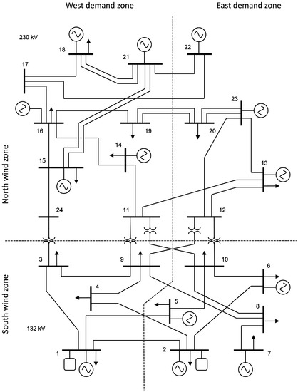
Figure 1.
Modified version of the IEEE RTS.
We consider that wind-power production and demand vary according to the area of the power system in which they are located. The historical data of electricity demand and wind-power production have been taken from [24] for the year 2016. The daily evolution of electricity demand for the loads located in the western and eastern zones is shown in Figure 2 and Figure 3, respectively, while the daily evolution of wind-power production in the northern and southern zones of the power system is shown in Figure 4 and Figure 5, respectively. These figures show the minimum and maximum values of electricity demand and wind-power production at different zones. Moreover, note that, while the daily electricity demand follows a clear pattern, the daily wind-power production does not. Note also that each curve of Figure 2, Figure 3, Figure 4 and Figure 5 represents a different day of the year 2016.
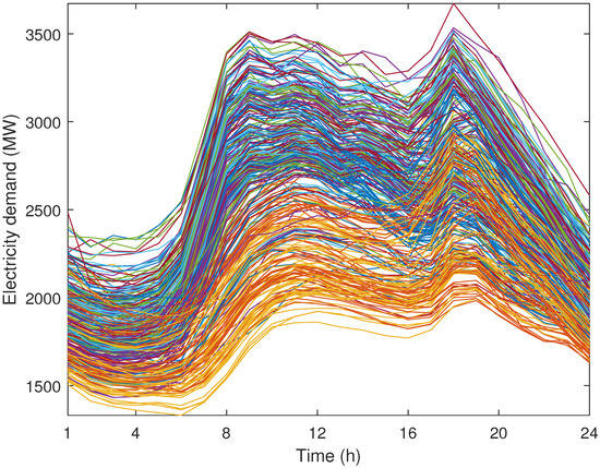
Figure 2.
Case study: daily evolution of electricity demand in the western zone during a year.
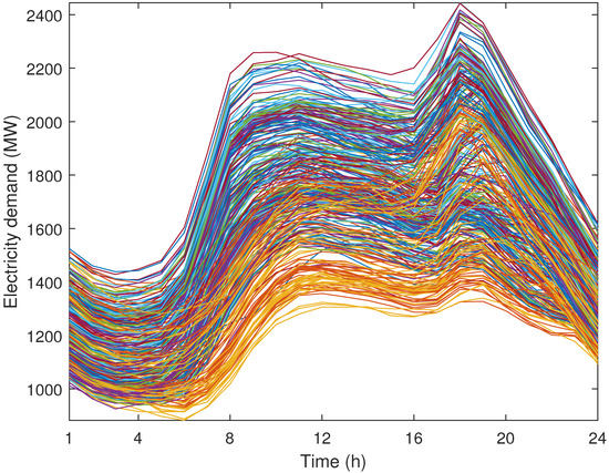
Figure 3.
Case study: daily evolution of electricity demand in the eastern zone during a year.
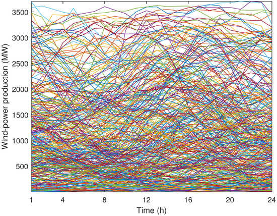
Figure 4.
Case study: daily evolution of wind-power production in the northern zone during a year.
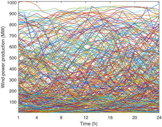
Figure 5.
Case study: daily evolution of wind-power production in the southern zone during a year.
We work with hourly data, thus the duration of time steps, , is one hour. The efficiency of the storage units in charging and discharging is considered to be equal to 90%. The energy initially stored in storage units is assumed to be zero for all representative days. Bus 1 is the reference bus of the optimization problem and we consider a base power of 100 MW. We consider a total investment budget of $20,000 million, which is higher than the sum of the investment costs of all candidate units. Therefore, the total investment budget does not limit the investment decisions of the G&TEP problem. Annualized investment costs are 10% of the total costs.
3.2. Results
As previously explained, the use of representative days reduces the computational effort in power-system planning problems representing historical data without losing accuracy. For that reason, we first normalize the historical data of Figure 2, Figure 3, Figure 4 and Figure 5 and then use the resulting curves as input data for the K-means methods described in Section 2 obtaining the parameters and , which respectively represent the capacity factor of wind-power unit w and the demand factor of load d on representative day r and hour h. Since we normalize the input data, the values of these parameters are between 0 and 1. It is worth mentioning that we obtain different values of parameters for wind-power production in the northern and southern zones as well as different values of parameters for the loads located in the western and eastern zones of the power system. Furthermore, for the sake of simplicity, we assume that, within each zone, the values of the parameters and for each representative day and hour are the same for all wind-power units and loads, respectively. In the case of applying the MKM with and to the historical data in Figure 2, Figure 3, Figure 4 and Figure 5, we obtain the 10 (2 × 5) representative days of electric demand in the western and eastern zones depicted in Figure 6 and Figure 7, respectively, while the 10 representative days of wind-power production in the northern and southern zones are represented in Figure 8 and Figure 9, respectively. Additionally, the values of parameters , which represent the weight of each representative day, are provided in Table 1.
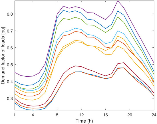
Figure 6.
Case study: representative days of electric demand in the western zone obtained using the modified K-means method with and .
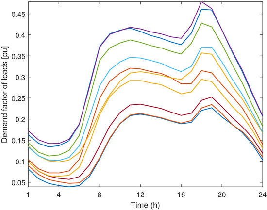
Figure 7.
Case study: representative days of electric demand in the eastern zone obtained using the modified K-means method with and .

Figure 8.
Case study: representative days of wind-power production in the northern zone obtained using the modified K-means method with and .
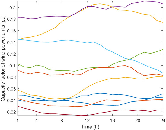
Figure 9.
Case study: representative days of wind-power production in the southern zone obtained using the modified K-means method with and .

Table 1.
Case study: weight of representative days obtained using the modified K-means method with and .
It should be mentioned that the demand values in the western zone are greater than in the eastern zone, as can be observed in Figure 2 and Figure 3. In addition, the wind-power production values are associated with the northern zone, as illustrated in Figure 4 and Figure 5. Both of these results can be observed in Figure 6, Figure 7, Figure 8 and Figure 9, where representative days with the parameters and are represented, since the normalization process for the input data was carried out considering the historical data from all zones. It is expected that the need to supply the high demands in the western zone will condition the investment decisions of the expansion problem.
3.3. Validation
First of all, we solve the G&TEP problem using all the historical data to find the so-called exact solution in order to compare it with the results obtained using representative days provided by both K-means methods set out in Section 2. For that purpose, we have implemented the approach described in Appendix A with the changes detailed in Appendix B.
The G&TEP problem is solved taking the 366 days of the year 2016 as historical data. The annualized investment cost, , rises to $682 million, while the total annualized cost, , is $3124 million. The results show that 0.14% of the total demand is not supplied. The computational time required to obtain the exact solution is 36 h 56 min.
Next, for assessment purposes, we have implemented the model presented in Appendix A using representative days as follows:
- Step 1: Solve the G&TEP problem using the representative days obtained through clustering methods for different values of the parameter K.
- Step 2: Set the values of the expansion planning decision variables (, ; , ; , ; , ) obtained at Step 1 and solve the G&TEP problem using all the historical data.
- Step 3: Calculate the percentage error, , associated with the total annualized cost obtained at Step 2, , with regard to the total annualized cost provided by the exact solution, , using Equation (2):
These steps are followed in the case study using a set of values of the parameter K which range from 10 to 80, where the maximum value which could be chosen was 366. This means that we work with an equivalent quantity of data ranging from 3 to 22% of all the historical data considered.
Simulations have been implemented on a Gigabyte R280-A3C with 2 Intel Xeon E5-2698 at 2.3 GHz and 256 GB of RAM using CPLEX 12.7.0.0 [25] under GAMS 24.8.3 [26].
The results are summarized in Table 2, where and denote the annualized investment cost obtained at Step 1 and the total annualized cost obtained at Step 2, respectively, represents the error associated with the total annualized cost defined in (2), and the last two columns show the computational time required for solving the problem set out at Step 1. It should be noted that the investment costs shown in Table 2 are different depending on the value of K and the clustering method selected, which means that the investment decisions obtained at Step 1 are different for each of the cases analyzed.
Table 2.
Case study: analysis of the results obtained from the clustering methods.
Figure 10 depicts the total annualized cost obtained using several values of K and for each of the two clustering methods. It is worth mentioning that we define the value of K when we use the TKM while we fix the values of and when we apply the MKM. In order to compare the results obtained using the two clustering methods, we have chosen the values of and , which can be seen in [23], taking into account Equation (1). As can be observed, the total annualized costs for the MKM are closer to the exact solution than those obtained using the TKM for all the cases evaluated. Note that the differences between the results obtained using the clustering methods and the exact solution generally decrease at the same time that the value of K increases.
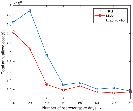
Figure 10.
Case study: total annualized cost obtained using different values of K and clustering methods.
As observed in Table 2, the errors associated with the MKM are always lower than those obtained using the TKM for all the cases analyzed, especially in those where the parameter K presents a small value. In particular, the case analyzed using with the MKM returns an error of 0.01%. This is because the expansion plan of the solution obtained in this case is to build all candidate conventional generating units and wind-power units at maximum capacity, all candidate storage units, and all transmission lines except for one of them, while the expansion plan of the exact solution is the same, with the difference that two candidate transmission lines are not built.
Regarding the resolution of the G&TEP problem using representative days (Step 1), the TKM generally provides shorter computational times, especially in those cases where parameter K presents a high value, although the differences are in no case significant.
Taking into account the results shown in Table 2, the MKM leads to lower values of total annualized cost and than the TKM. Although the computational times obtained using the MKM are generally greater than those acquired using the TKM, the difference between the two methods is not very large, and in fact they are reasonable times for a planning problem. Thus, the expansion plan using MKM outperforms the investment scheme considering TKM.
4. Conclusions
This paper proposes a new clustering method to generate operating conditions for making expansion planning decisions in power systems. As a distinctive feature, the proposed method allows an adequate characterization of the maximum and minimum values of the input data. In addition, we arrange the operating conditions obtained using the K-means method into representative days in order to represent the chronology of the historical data. This allows us to include storage units in expansion planning problems.
From numerical results of using the MKM to solve the G&TEP problem, we conclude that for a given number of representative days the MKM provides a solution closer to the exact solution than that provided by the TKM. Note that the origin of these differences is in the fact that investment decisions change depending on the clustering method chosen to obtain the representative days. Furthermore, for a given clustering technique, either TKM or MKM, investment decisions change if we modify the value of parameter K or parameters and , respectively. This is expected since the use of a large number of representative days usually leads to a more accurate solution. Additionally, the MKM also outperforms the TKM in terms of computational times needed to achieve the solution of the G&TEP problem for a given error with regard to the total annualized cost provided by the exact solution.
Author Contributions
Conceptualization, Á.G.-C., L.B. and R.G.-B.; methodology, Á.G.-C. and L.B.; software, Á.G.-C.; validation, Á.G.-C.; formal analysis, Á.G.-C., L.B. and R.G.-B.; investigation, Á.G.-C., L.B. and R.G.-B.; resources, Á.G.-C., L.B. and R.G.-B.; data curation, Á.G.-C.; writing—original draft preparation, Á.G.-C.; writing—review and editing, L.B. and R.G.-B.; visualization, Á.G.-C.; supervision, L.B. and R.G.-B.; project administration, L.B.; funding acquisition, L.B. All authors have read and agreed to the published version of the manuscript.
Funding
This research was funded by the Ministry of Science, Innovation, and Universities of Spain under Projects RTI2018-096108-A-I00 and RTI2018-098703-B-I00 (MCIU/AEI/FEDER, UE), and the Universidad de Castilla-La Mancha under Grant 2019-UNIVERS-9385.
Conflicts of Interest
The authors declare no conflict of interest. The funders had no role in the design of the study; in the collection, analyses, or interpretation of data; in the writing of the manuscript, or in the decision to publish the results.
Notations
The main notation used in this paper is stated below for quick reference, while other symbols are defined as needed throughout the text. A subscript r/h in the symbols below denotes their values in the rth representative day/hth hour:
| Indices | |
| d | Load |
| g | Conventional generating unit |
| h | Hour |
| ℓ | Transmission line |
| n | Bus |
| r | Representative day |
| s | Storage facility |
| w | Wind-power unit |
| Receiving bus of transmission line ℓ | |
| Destination bus of transmission line ℓ | |
| Sets | |
| Set of indexes d of loads connected to bus n | |
| Set of indexes d of loads | |
| Set of indexes g of conventional generating units connected to bus n | |
| Set of indexes g of conventional generating units | |
| Set of indexes g of candidate conventional generating units | |
| Set of indexes h of hours | |
| Set of indexes ℓ of transmission lines | |
| Set of indexes ℓ of candidate transmission lines | |
| Set of indexes n of buses | |
| Set of indexes r of representative days | |
| Set of indexes s of storage units connected to bus n | |
| Set of indexes s of storage units | |
| Set of indexes s of candidate storage units | |
| Set of indexes w of wind-power units connected to bus n | |
| Set of indexes w of wind-power units | |
| Set of indexes w of candidate wind-power units | |
| Parameters | |
| Susceptance of transmission line ℓ [] | |
| Operation cost coefficient of conventional generating unit g [$/MWh] | |
| Load-shedding cost coefficient of load d [$/MWh] | |
| Energy initially stored in storage facility s [MWh] | |
| Maximum level of energy of storage facility s [MWh] | |
| Investment cost coefficient of candidate conventional generating unit g [$/MW] | |
| Annualized investment cost coefficient of candidate conventional generating unit g [$/MW] | |
| Investment cost coefficient of candidate transmission line ℓ [$] | |
| Annualized investment cost coefficient of candidate transmission line ℓ [$] | |
| Investment cost coefficient of candidate storage facility s [$] | |
| Annualized investment cost coefficient of candidate storage facility s [$] | |
| Investment cost coefficient of candidate wind-power unit w [$/MW] | |
| Annualized investment cost coefficient of candidate wind-power unit w [$/MW] | |
| Total investment budget [$] | |
| Maximum number of units that can be built of candidate storage facility s | |
| Peak power consumption of load d [MW] | |
| Capacity of conventional generating unit g [MW] | |
| Power flow capacity of transmission line ℓ [MW] | |
| Charging power capacity of storage facility s [MW] | |
| Discharging power capacity of storage facility s [MW] | |
| Capacity of wind-power unit w [MW] | |
| Capacity factor of wind-power unit w [pu] | |
| Demand factor of load d [pu] | |
| Duration of time steps [h] | |
| Charging efficiency of storage facility s | |
| Discharging efficiency of storage facility s | |
| Weight of representative day r [days] | |
| Optimization Variables | |
| Energy stored in storage facility s [MWh] | |
| Number of units to be built of candidate storage facility s | |
| Power produced by conventional generating unit g [MW] | |
| Capacity to be built of conventional generating unit g [MW] | |
| Power flow through transmission line ℓ [MW] | |
| Unserved demand of load d [MW] | |
| Charging power of storage facility s [MW] | |
| Discharging power of storage facility s [MW] | |
| Power produced by wind-power unit w [MW] | |
| Capacity to be built of wind-power unit w [MW] | |
| Binary variable that is equal to 1 if candidate transmission line ℓ is built, being 0 otherwise | |
| Voltage angle at bus n [rad] | |
Appendix A. Formulation of the Generation and Transmission Expansion Planning Problem
The purpose of the G&TEP problem is to minimize the operation costs along with the costs incurred in building new facilities (generating units, storage units, and transmission lines). In this section, we provide the formulation of the G&TEP problem with a deterministic approach using the following mixed-integer nonlinear programming (MINLP) model:
subject to
where variables in set , ; , , , ; , ; , , , ; , , , ; , , , , , ; , , , ; , ; , ; , , , are the optimization variables of problem (A1).
The objective function (A1a) represents the aim of the G&TEP problem, which is to minimize the investment (generation, storage, and transmission facilities) and operating (power produced by conventional generating units and unserved demand) costs. The terms associated with operating costs are multiplied by the weight of the corresponding representative day, , to make them comparable to expansion costs. Note that the sum of over all representative days is 365, i.e., the total number of days in a year.
Constraints (A1b) limit the number of units of each candidate storage facility to be built. Constraints (A1c) define , , as integer variables. Constraints (A1d)–(A1e) impose bounds on the capacity of conventional and wind-power generating units, respectively, to be built. Constraints (A1f) define as binary variables that indicate whether a candidate transmission line is built () or not (). Constraint (A1g) imposes total investment budget for building candidate conventional generating units, transmission lines, storage, and wind-power units. Constraints (A1h)–(A1ab) are the operation constraints and consist of Equation (A1h), which impose the power balance at each bus, where demand factors , , , , are linked to the output of the K-means method described in Section 2; constraints (A1i)–(A1j), which define the power flows through existing and candidate transmission lines, respectively, which are limited by constraints (A1k); Equation (A1l), which define the energy stored in storage units for all representative days and hours, excluding the first hour of each day; Equations (A1m)–(A1n) that define the energy stored in existing and candidate storage units, respectively, for the first hour of all representative days; constraints (A1o)–(A1p), which ensure that existing and candidate storage units, respectively, store a minimum amount of energy at the end of each representative day; constraints (A1q)–(A1r), which limit the energy stored in the existing and candidate storage units, respectively; constraints (A1s)–(A1t), which set the generation limits for existing and candidate conventional generating units, respectively; constraint (A1u), which limits the load shedding; constraints (A1v)–(A1w), which impose bounds on the charging power of existing and candidate storage units, respectively; constraints (A1x)–(A1y), which impose bounds on the discharging power of existing and candidate storage units, respectively; constraints (A1z)–(A1aa) that set the generation limits by existing and candidate wind-power units, respectively, where wind-power capacity factors , , , , are associated with the output of the K-means method described in Section 2; and constraints (A1ab), which define the voltage angle at the reference bus.
It is important to mention that the network constraints are modeled on the G&TEP problem using a DC model without losses for the sake of simplicity. In addition, fixed costs are not considered and the capacity of each generating unit to be installed, i.e., the variables , ; and , , are considered to be continuous.
The G&TEP problem (A1) is an MINLP model. Nonlinear terms are in constraints (A1j), i.e., products of binary and continuous variables. These nonlinear terms can be replaced by exact equivalent mixed-integer linear expressions as explained, e.g., in [27]. Thus, the G&TEP problem (A1) can ultimately be formulated as a mixed-integer linear programming model that can be solved using available branch-and-cut solvers, e.g., CPLEX [25].
Appendix B. Formulation of the G&TEP Problem Considering All Historical Data
Solving the G&TEP problem considering all historical data leads to some changes in the formulation of problem (A1), in order to properly characterize the continuity in time of the historical data. Constraints (A1m)–(A1p) are replaced by constraints (A2)–(A4), where constraint (A2) alludes to the energy stored in each storage unit during the first hour of all the days except the first one, relating it to the energy stored in the same storage unit during the last hour of the previous day; and constraints (A3)–(A4) refer to the energy stored in each existing and candidate storage unit, respectively, during the first hour of the first day, linking it to the energy initially stored in the same storage unit on the first day, :
References
- Morales, J.M.; Baringo, L.; Conejo, A.J.; Mínguez, R. Probabilistic power flow with correlated wind sources. IET Gener. Transm. Distrib. 2010, 4, 641–651. [Google Scholar] [CrossRef]
- Xie, L.; Carvalho, P.M.S.; Ferreira, L.A.F.M.; Liu, J.; Krogh, B.H.; Popli, N.; Ilić, M.D. Wind integration in power systems: Operational challenges and possible solutions. Proc. IEEE 2011, 99, 214–232. [Google Scholar] [CrossRef]
- Bell, W.P.; Wild, P.; Foster, J.; Hewson, M. Wind speed and electricity demand correlation analysis in the Australian National Electricity Market: Determining wind turbine generators’ ability to meet electricity demand without energy storage. Econ. Anal. Policy 2015, 48, 182–191. [Google Scholar] [CrossRef][Green Version]
- Poulin, A.; Dostie, M.; Fournier, M.; Sansregret, S. Load duration curve: A tool for technico-economic analysis of energy solutions. Energy Build. 2008, 40, 29–35. [Google Scholar] [CrossRef]
- Hoppner, F.; Klawonn, F.; Kruse, R.; Rumkler, T. Fuzzy Cluster Analysis; Wiley: Chichester, UK, 1999. [Google Scholar]
- Ramezani, M.; Singh, C.; Haghifam, M.R. Role of clustering in the probabilistic evaluation of TTC in power systems including wind power generation. IEEE Trans. Power Syst. 2009, 24, 849–858. [Google Scholar] [CrossRef]
- Baringo, L.; Conejo, A.J. Correlated wind-power production and electric load scenarios for investment decisions. Appl. Energy 2013, 101, 475–482. [Google Scholar] [CrossRef]
- Caramanis, M.; Tabors, R.; Nochur, K.S.; Schweppe, F. The introduction of non-dispatchable technologies a decision variables in long-term generation expansion models. IEEE Trans. Power App. Syst. 1982, PAS-101, 2658–2667. [Google Scholar] [CrossRef]
- Wogrin, S. Generation Expansion Planning in Electricity Markets with Bilevel Mathematical Programming Techniques. Ph.D. Thesis, Universidad Pontificia Comillas de Madrid, Madrid, Spain, 2013. [Google Scholar]
- Baringo, L.; Conejo, A.J. Transmission and wind power investment. IEEE Trans. Power Syst. 2012, 27, 885–893. [Google Scholar] [CrossRef]
- Montoya-Bueno, S.; Muñoz, J.I.; Contreras, J. A stochastic investment model for renewable generation in distribution systems. IEEE Trans. Sustain. Energy 2015, 6, 1466–1474. [Google Scholar] [CrossRef]
- Baringo, L.; Conejo, A.J. Wind power investment within a market environment. Appl. Energy 2011, 88, 3239–3247. [Google Scholar] [CrossRef]
- Baringo, L.; Conejo, A.J. Strategic wind power investment. IEEE Trans. Power Syst. 2014, 29, 1250–1260. [Google Scholar] [CrossRef]
- Domínguez, R.; Conejo, A.J.; Carrión, M. Toward fully renewable electric energy systems. IEEE Trans. Power Syst. 2015, 30, 316–326. [Google Scholar] [CrossRef]
- Dehghan, S.; Amjady, N. Robust transmission and energy storage expansion planning in wind farm-integrated power systems considering transmission switching. IEEE Trans. Sustain. Energy 2016, 7, 765–774. [Google Scholar] [CrossRef]
- Nogales, A.; Wogrin, S.; Centeno, E. Impact of technical operational details on generation expansion in oligopolistic power markets. IET Gen. Trans. Dist. 2016, 10, 2118–2126. [Google Scholar] [CrossRef]
- Wogrin, S.; Dueñas, P.; Delgadillo, A.; Reneses, J. New approach to model load levels in electric power systems with high renewable penetration. IEEE Trans. Power Syst. 2014, 29, 2210–2218. [Google Scholar] [CrossRef]
- Hemmati, R.; Hooshmand, R.-A.; Khodabakhshian, A. Comprehensive review of generation and transmission expansion planning. IET Gener. Transm. Distrib. 2013, 7, 955–964. [Google Scholar] [CrossRef]
- Spyrou, E.; Ho, J.; Hobbs, B.; Johnson, R.; McCalley, J. What are the benefits of co-optimizing transmission and generation investment? Eastern interconnection case study. IEEE Trans. Power Syst. 2017, 32, 4265–4277. [Google Scholar]
- Conejo, A.J.; Baringo, L.; Kazempour, S.J.; Siddiqui, A.S. Investment in Electricity Generation and Transmission; Springer: Cham, Switzerland, 2016. [Google Scholar]
- Zhou, Y.; Wang, L.; McCalley, J.D. Designing effective and efficient incentive policies for renewable energy in generation expansion planning. Appl. Energy 2011, 88, 2201–2209. [Google Scholar] [CrossRef]
- Grigg, C.; Wong, P.; Albrecht, P.; Allan, R.; Bhavaraju, M.; Billinton, R.; Chen, Q.; Fong, C.; Haddad, S.; Kuruganty, S.; et al. The IEEE Reliability Test System-1996. A report prepared by the Reliability Test System Task Force of the Application of Probability Methods Subcommittee. IEEE Trans. Power Syst. 1999, 14, 1010–1020. [Google Scholar] [CrossRef]
- García-Cerezo, Á.; Baringo, L.; García-Bertrand, R. Representative Days for Expansion Decisions in Power Systems: Data for the Case Study. Available online: https://drive.google.com/open?id=15svP0AU7rAplfTKkscEqshAo414f7T06 (accessed on 13 November 2019).
- Energinet—Energy Data Service. Available online: http://www.energidataservice.dk/ (accessed on 13 October 2019).
- The ILOG CPLEX. Available online: http://www.ilog.com/products/cplex/ (accessed on 13 October 2019).
- Rosenthal, R.E. GAMS, A User’s Guide; GAMS Development Corporation: Washington, DC, USA, 2012. [Google Scholar]
- Floudas, C.A. Nonlinear and Mixed-Integer Optimization: Fundamentals and Applications; Oxford University Press: New York, NY, USA, 1995. [Google Scholar]


© 2020 by the authors. Licensee MDPI, Basel, Switzerland. This article is an open access article distributed under the terms and conditions of the Creative Commons Attribution (CC BY) license (http://creativecommons.org/licenses/by/4.0/).