Article

A Novel Fault Classification Approach for Photovoltaic Systems

by
Varaha Satya Bharath Kurukuru
1,
Frede Blaabjerg
2,*,
Mohammed Ali Khan
1 and
Ahteshamul Haque
1
1
Advance Power Electronics Research Laboratory, Department of Electrical Engineering, Jamia Millia Islamia (A Central University), New Delhi 110025, India
2
Department of Energy Technology, Aalborg University, 9220 Aalborg, Denmark
*
Author to whom correspondence should be addressed.
Energies 2020, 13(2), 308; https://doi.org/10.3390/en13020308
Submission received: 5 December 2019 / Revised: 24 December 2019 / Accepted: 7 January 2020 / Published: 8 January 2020
(This article belongs to the Special Issue Emerging Photovoltaic Technology in Northern Europe)

Abstract

:
Photovoltaic (PV) energy has become one of the main sources of renewable energy and is currently the fastest-growing energy technology. As PV energy continues to grow in importance, the investigation of the faults and degradation of PV systems is crucial for better stability and performance of electrical systems. In this work, a fault classification algorithm is proposed to achieve accurate and early failure detection in PV systems. The analysis is carried out considering the feature extraction capabilities of the wavelet transform and classification attributes of radial basis function networks (RBFNs). In order to improve the performance of the proposed classifier, the dynamic fusion of kernels is performed. The performance of the proposed technique is tested on a 1 kW single-phase stand-alone PV system, which depicted a 100% training efficiency under 13 s and 97% testing efficiency under 0.2 s, which is better than the techniques in the literature. The obtained results indicate that the developed method can effectively detect faults with low misclassification.

1. Introduction

The increasing energy demands of modern society raise significant environmental concerns. Hence, substantial research on renewable energy technologies is important for realizing the potential of cleaner energy resources [1]. Among the major renewable energy systems, solar energy is the most abundant, inexhaustible, and cleanest during operation [2]. Moreover, the progress in solar energy technologies and improving efficiency made photovoltaic (PV) systems a dominant player in the global electricity production market [3]. However, they have failed under many occasions, due to recurring undetectable faults [1]. In general, faults in a PV system are classified depending on the location of the fault, i.e., AC stage or DC stage. The AC faults include gating and switching failures, open and short circuit switches [4], and filter failure-inducing harmonics in the circuits. Whereas DC faults include various module-based faults [5], failure of maximum power-point tracking (MPPT) algorithms, and faults associated with DC-DC converters [6,7]. Also, MPPT systems are responsible for injecting maximum power into the circuit. During high irradiation intensity, increased power on the input side may cause false tripping of over-current relays [8,9]. In addition, non-linear characteristics of PV array makes it difficult to attain a decision boundary for the faulty condition [10]. The faults occurring on the DC side can have catastrophic impacts on the AC side if they remain undetected, which leads to fire Hazards or reduction in output power. In order to overcome these effects, continuous real-time monitoring and fault classification is necessary to improve the life and efficiency of the PV systems.
Conventionally, many signal processing techniques were adapted by the researchers to observe the patterns of faults at different levels of PV systems [11]. These techniques involve many steps like signal conditioning for denoising, input normalization such that the input values exist within the realm of the capabilities of the selected algorithms, and feature extraction for enhancement of the separability of the classes. Apart from signal processing techniques, classification algorithms were also considered for analyzing the anomalies. Over the past years, many fault classification and anomaly detection algorithms were studied and implemented, but machine learning-based algorithms proved to be more effective. One of the methods, as introduced in [12], discusses the support vector machine (SVM) algorithm, which creates a decision boundary to predict whether a certain fault has occurred or not. However, they face a disadvantage in the selection of features, which, when done by trial and error method, may lead to the faulty output. An improved method of supervised learning, as discussed in [13], introduces artificial neural networks (ANN) for predicting outputs and identifying faults in a PV system. But it has been observed that they undergo problems of overfitting and often fail to predict under test data. Besides, ANNs are computationally bulky and expensive to train. Certain advanced versions of ANNs like multilayer perceptron networks (MLPN) and backpropagation algorithms were introduced to overcome problems of ANNs and for enhanced accuracy.
Contrarily, a system can be subjected to a large number of undefined faults that are new to the system. In such a case, an approach to supervised learning fails to encompass the condition. In order to overcome the difficulty, a semi-supervised learning algorithm, which not only detects faults but also identifies possible fault types, was introduced in [14] to speed up system recovery. In this approach, two known parameters were chosen as a center for clustering and the unknown faults were grouped based on the vicinity to these clusters. The drawback associated with these systems is that they are challenging to implement for large PV systems and also face difficulties due to overlapping amongst different clusters. To overcome this, a comprehensive unsupervised learning technique that manually assigns weight using a kernel-based approach with only one hidden unit was introduced in [15]. The radial based functions used in the kernel method creates a decision boundary by importing data into a high dimensional feature space and then converting them back into two-dimensional data. This is achieved by calculating the Euclidean distance between landmarks and training data set and operating on parameter kernel radius for deciding the spread of the function. Even this operation fails to distinguish between two points that are at an equal distance and reasonably gave an error in the exactness as to where a certain dataset belonged. Further, an improved variant, including a cosine component, was introduced to supplement and overcome the Euclidean distance problem [16]. Here, the cosine component distinguishes between two similar data sets that were aligned at equal distances but at different angles. However, manually assigning weights remained a complex task requiring a lot of human efforts.
From the above discussion, the problem at hand is to develop an enhanced technique over prevalent practices to classify faults in single-phase PV systems. The literature provided various techniques to overcome the problem, but each of them tends to be primitive and computationally complex. Apart from this, the inability of classification approaches to handle large amounts of data, complex pre-processing steps, and inability to discriminate among the patterns in the data needs attention.
In this paper, a new classification process, as depicted in Figure 1, is developed. Various faults associated with PV systems were simulated, and their effect on the voltage and current outputs were identified. Here, the data acquisition plays a major role in storing all the data corresponding to different faults and operating conditions of the PV system. Further, the keen points of the identified outputs were analyzed using wavelet transform, and the corresponding features were extracted. The extracted features were subjected to classification by developing a new RBFN classifier. The developed algorithm assigns weights adaptively in the consecutive layers and performs efficient clustering to develop an efficient fault classifier. The developed classifier is introduced in a feedforward mode with the PV system to classify the increased number of faults efficiently.
The further sections of the paper provide a detailed explanation of the fault classification procedure. Section 2 identifies various faults that affect the operation of a PV system. Section 3 describes the signal pre-processing and feature extraction process using wavelet analysis. Section 4 explains the pattern recognition and classification technique by developing a dynamically fused kernel for RBFN. Finally, the extracted features and the kernel network are adapted together for developing a fault classifier for a single-phase stand-alone photovoltaic system in Section 5. The final simulation results and comparison with literature work depicts the feasibility of the developed procedure in classifying PV system faults within a stipulated time.

2. PV System Faults

PV systems are subjected to a variety of faults, impacting the output power of the system. In general terms, the faults observed in any system are classified under three categories, early failures, intrinsic or random failure, and wear out [17].
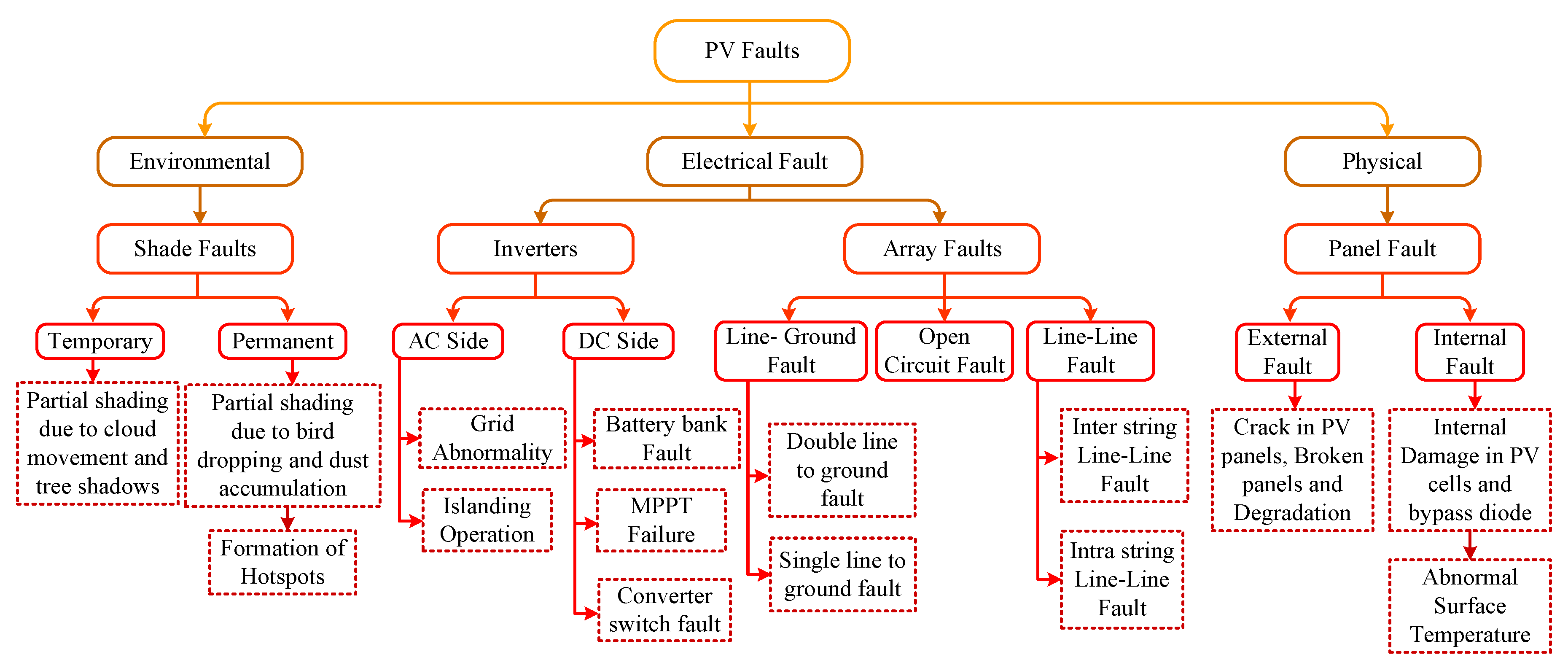
Figure 2 depicts some very serious faults that occur in PV systems. Generally, these faults can be classified into three categories: early faults, extrinsic faults, and deterioration stage. The early failures are observed during the initial stages of the installation and operation of PV systems. Any defect or flaw in the PV module or the power electronic converters results in a quick degradation; hence, it decreases the service life of the system. The module faults and the cable failures are observed to share a major part of the early failure cases. Extrinsic failures are the midlife failures observed in a PV system [18]. It was predicted that 2% of the PV modules do not comply with the specifications of the manufacturer after a certain span of operation. Various studies have shown that interconnection defects and module glass breakage failures are the major causes of extrinsic failures. The deterioration stage or wear out failure occurs at the end of the life span and is the most common scenario that can be observed in PV systems. The operation or the life of the PV system is concealed whenever a safety problem or power drop occurs. There are a lot of studies analyzing different issues present in PV systems [19,20], demonstrating an interest in detecting faults to the greatest extent as early as possible. A brief overview of different faults, their potential causes, and effects were depicted in Table 1.

3. Feature Extraction Methodology

Every fault condition and operation in a PV system has a specific impact on the output voltage and current. This causes a difference in the waveform or signal of the outputs when compared to a normal operating scenario. These changes or disturbances have different features when observed in the time and frequency domains. Generally, wavelet analysis [21] is known to give benefits with simultaneous time and frequency localization and has seen recent application to feature extraction in pattern recognition problems.

Wavelet Transform

Wavelet transform (WT) is a spectral analysis method, which decomposes a signal into a set of oscillatory functions called wavelets. The wavelets are localized in time, and thus, WT provides a time-frequency representation. Considering a time-domain signal f ( t ) in any L 2 ( R ) space of square-integrable functions [22], which can be formulated using a family of orthonormal wavelet functions, the wavelet transformation of the signal is given by:
[ W ψ f ] ( s , τ ) = 1 | s | R f ( t ) ψ * ( t τ s ) d t
where ψ ( t ) is the mother wavelet, s = 1 ,   , m and τ = 1 ,   ,   n are the scale and translation parameters, respectively; [ W ψ f ] ( s ,   τ ) is the wavelet transformation of the signal f ( t ) [23].
There are two basic ways in which a wavelet can be manipulated, the first one is the translation of the wavelet, and the second one is the scaling of the wavelet. The translation corresponds to movements along the time axis, and scaling refers to the spreading out of the wavelet. These two basic manipulations are used in the discrete wavelet transform (DWT) of the signal, which means that the DWT is implemented at several locations of the signal, and for several scales of the wavelet, with the purpose to capture features that are local in time and local in frequency. Generally, wavelets are chosen depending on the nature of the observed signal of interest and the aim of the analysis. For a function to be transformed into a wavelet, some conditions must be achieved, such as admissibility condition, integration to zero, and unit energy [24].
The wavelet function at scale a and location b is defined as:
Ψ a , b ( t ) = 1 a Ψ ( t a b )
where, a and b are the dilation (or scale) and translation (or shifting) parameters, respectively.
If discrete values of parameters a and b are considered, the wavelet function may be rewritten by using a logarithmic discretization of the a scale and making location b proportional to that a scale. This modification leads to a discrete version of the wavelet function, which has the form:
Ψ m , n ( t ) = 1 a 0 m Ψ ( t n b 0 a 0 m a 0 m )
where, m is the discrete dilation parameter; n is the discrete translation parameter; a 0 : is a fixed dilation step parameter; b 0 : is a fixed translation step parameter
Parameters m and n are contained in the set of integers . Parameter a 0 must be greater than 1 because of the stability of Ψ m , n ( t ) (as m→∞ then a 0 m 0 and Ψ m , n ( t ) ), and parameter b 0 must be greater than 0 since otherwise no wavelet translations could be performed. In addition, note that the size of the translation steps is proportional to the wavelet scale a 0 m through the relationship Δ b = b 0 a 0 m .
Setting a o = 2 and b o = 1 in (3) leads to an arrangement known as the dyadic grid, which is a power-of-two arrangement for both the dilation and translation steps, and is given by:
Ψ m , n ( t ) = 1 2 m Ψ ( t n 2 m 2 m )
where, Ψ 0 , 0 ( t ) = Ψ ( t ) is known as the mother wavelet function.
The DWT of a discrete signal x(t) using discrete wavelets is given by:
T m , n = t = 0 N 1 x ( t ) 1 2 m Ψ ( t n 2 m 2 m ) x , Ψ m , n
where, N is the length of the discrete signal x(t); T m , n are the detailed wavelet coefficients for a scale-location grid of index m, n.
The DWT may be viewed as the convolution of the signal x(t) with dilated and translated versions of the mother wavelet, by which the wavelet coefficients T m , n at all scale-location indices m, n can be obtained. Likewise, the original signal x(t) can be reconstructed through the wavelet coefficients T m , n , using the inverse discrete wavelet transform, which is defined as:
x ( t ) = m = 1 M n = 0 2 M 1 T m , n Ψ m , n ( t )
where, M = ln ( N ) ln ( 2 ) is the number of iterations that can be computed and N = 2 M is the length of the discrete input signal x ( t ) .
Equations (5) and (6) may be described as a decomposition-reconstruction process summarized as follows:
Decomposition process:
x ( t )   x , Ψ m , n T m , n
Reconstruction process:
x ( t )   m = 1 M n = 0 2 M 1 x , Ψ m , n Ψ m , n ( t ) T m , n
In general, Orthonormal dyadic discrete wavelets are associated with scaling and wavelet functions, which are related to smoothing of a signal and the extraction of high signal frequencies. Analogously to the process to obtain the wavelet coefficients T m , n (5), the signal x(t) can be convoluted with dilated and translated versions of the father wavelet, to obtain the approximation coefficients S m , n at all scale-location indices m, n as follow:
S m , n = t = 0 2 M 1 x ( t ) 1 2 m ( t n 2 m 2 m ) x ,   m , n
where, S m , n is the approximation coefficient for a scale-location grid of index m, n.
Once the signal is discretized, it is decomposed based on the mother wavelet chosen. The process of decomposition, reconstruction, and feature extraction were carried out to develop a feature matrix. The developed feature matrix is further subject to the classification process, which is explained in the next sections.

4. Pattern Classification Using RBFN

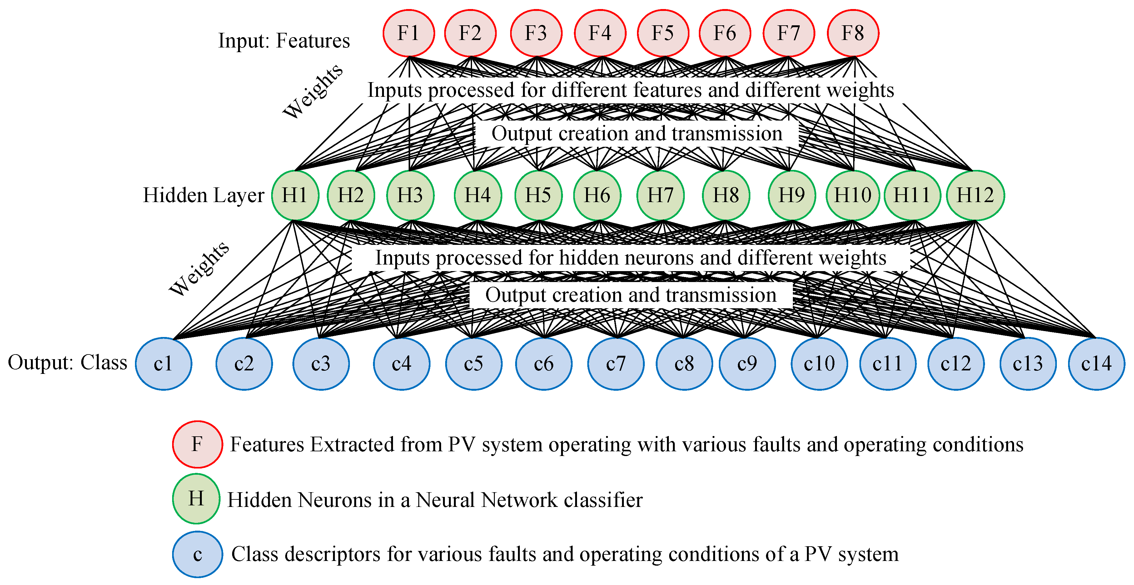
The RBFN [25] architecture is formed by combining three layers: the input layer, the non-hidden layer, and a linear output layer. Figure 3 represents the architecture of different layers in RBFN where Z n 0 } is an input vector. Considering the input vector, the overall mapping m : n 0 1 , of RBFN is depicted as:
f ( u ) = i = 1 n 1 x i θ i ( | | z z i | | ) + b
where n 1 is the total neurons in the hidden layer, Z i n 0 are the centers of RBFN, x i is the synaptic weights connecting hidden and output layer, b represents bias output layer, and the bias function is given by θ i for i t h hidden neuron.
Conventional RBFN’s employ multiple kernels like Gaussian [26], multiquadric [27], and inverse multiquadric [28]. The Gaussian kernel is the most commonly used kernel due to its versatility.
θ i ( | | z z i | | ) = exp ( | | z z i | | 2 σ 2 )
where, σ is the kernel radius of Gaussian.
In general, kernels measure the distance from clusters of the network. In the literature, Euclidean distance [29] is widely used as an efficient distance measurement technique. But the present-day researchers argue that the distance of the cosine kernel has more efficiency and complimentary properties when compared to the Euclidean distance measure.
θ i 1 ( z . z i ) = z . z i | | z | | | | z i | | + ξ
where, ξ > 0 is an insignificant constant in the denominator, which avoids the indeterminant form of (12) in any case of | | Z | | or | | Z i | | is zero. Accordingly, a new approach is developed by combining the Euclidean and cosine distances.
θ i ( z ,   z i ) = ω 1 θ i 1 ( z . z i ) + ω 2 θ i 2 ( | | z z i | | )
where θ i 1 ( z . z i ) , θ i ( | | z z i | | ) are the cosine and Euclidean kernels, respectively, with corresponding weights ω 1 and ω 2 .
By adapting the distinctive properties of cosine and Euclidean kernels, the developed system exhibited a significant improvement when compared to conventional RBFN kernel. But its observed that there is a manual fusion between the two kernels, and the weights ω 1 and ω 2 are adjusted using trial and error method. In general, while dealing with trial and error method, weights are equally assigned to the kernels. In order to overcome this drawback, a new framework is developed to optimize the weights with adaptive methods like the steepest descent method [30].
Let’s consider ω 1 and ω 2 to be dynamically adaptive variables:
ω 1 | ω 1 ( u ) | | ω 1 ( u ) | + | ω 2 ( u ) |
ω 2 | ω 2 ( u ) | | ω 2 ( u ) | + | ω 1 ( u ) |
where the normalization of mixing the weights ensure that ω 1 ( u ) + ω 2 ( u ) = 1 , the developed kernel can be formulated as:
θ i ( z , z i ) = | ω 1 ( u ) | θ i l ( z . z i ) + | ω 2 ( u ) | θ i 2 ( | | z z i | | ) | ω 1 ( u ) | + | ω 2 ( u ) |
The overall mapping at n t h learning linked to a specific epoch, can now be written as:
f ( u ) = i = 1 n 1 x i ( u ) θ i ( z ,   z i ) + b ( u )
where x i ( u ) depicts the synaptic weight and b ( u ) is the bias adapted at each iteration.
The cost function j ( u ) is given by:
j ( u ) = j ( ω 1 ( u ) ,   ω 2 ( u ) ) = 1 2 ( d 0 ( u ) f ( u ) ) 2
where d 0 ( u ) is the desired output at u t h iteration, ε ( u ) is the instantaneous error between the desired output and actual output as defined in (18).
ε ( u ) = d 0 ( u ) f ( u )
The updated rule for weights of the kernel is given by:
Δ ω 1 ( u ) = η j ( u ) ω 1 ( u )
By applying the chain rule differentiation for cost function analysis,
j ( u ) ω 1 ( u ) = j ( u ) ε ( u ) ε ( u ) f ( u ) f ( u ) θ i ( z , z i ) θ i ( z , z i ) ω 1 ( u )
By simplifying (19),
j ( u ) ω 1 ( u ) = ε ( u ) x i ( u ) | ω 1 ( u ) | | ω 2 ( u ) | ω 1 ( u ) [ | ω 1 ( u ) + ω 2 ( u ) | 2 ] × [ θ i 1 ( z . z i ) θ i 2 ( | | z z i | | ) ]
From (18) and (20), the updated rule for ω 1 ( u ) is depicted as:
ω 1 ( u + 1 ) = ω 1 ( u ) + η ε ( u ) x i ( u ) | ω 1 ( u ) | | ω 2 ( u ) | ω 1 ( u ) [ | ω 1 ( u ) | + | ω 2 ( u ) | ] 2 × [ θ i 1 ( z . z i ) θ i 2 ( | | z z i | | ) ]
For ω 2 ( u )
ω 2 ( u + 1 ) = ω 2 ( u ) + η ε ( u ) x i ( u ) | ω 1 ( u ) | | ω 2 ( u ) | ω 2 ( u ) [ | ω 1 ( u ) | + | ω 2 ( u ) | ] 2 × [ θ i 2 ( | | z z i | | ) θ i 1 ( z . z i ) ]
x i ( u + 1 ) = x i ( u ) + η ε ( u ) θ i ( z ,   z i )
b i ( u + 1 ) = b i ( u ) + η ε ( u )
Finally, the updated weights and bias are obtained from (24) and (25). It is observed that the developed approach does not require the prior assignment of weights due to its dynamic nature.

5. Methodology

5.1. System Layout and Data Collection

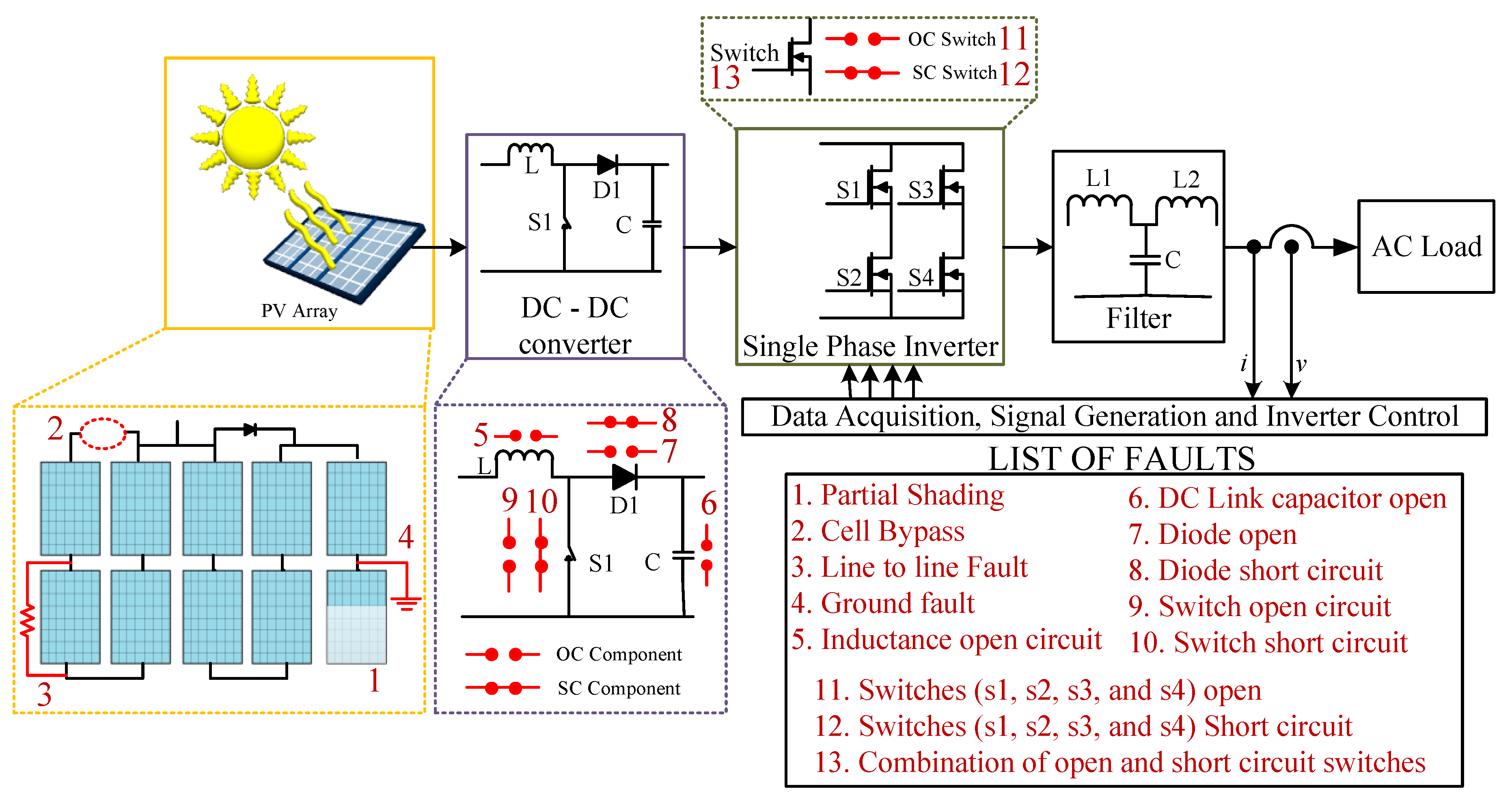
A simulation model of the single-phase two-stage standalone PV system [31] operating under standard test conditions of 1000   W / m 2 irradiance and 25 ° C temperature is developed using MATLAB/Simulink. The system includes a 1 kW PV array, a DC-DC boost converter, and an inverter fed from a 400 V dc obtained at the DC link [32]. The output of the PV system corresponds, 230 V RMS, 50 Hz AC, which is feeding a constant load and is isolated from the grid. For this study, the boost converter is operated with perturbation and observation MPPT algorithm, and the pulses to inverter switches are fed from a PWM generator operating at 10 kHz switching frequency [33]. The measured voltage and current are tabulated after each simulation run for every fault and operating condition.
The critical faults of the PV system, which are simulated in this experiment are depicted in Figure 4 and summarized in Table 2, and their description and effects are also detailed.
In this test, Daubechies ‘db5′ mother wavelet [34] has been chosen, and the fifth level of wavelet transform has been used to analyze due to its robustness, and it is least affected by the noise. The absolute value of wavelet coefficients and corresponding energy values are calculated by (27) show large change for every fault.
E = [ i = 1 i = N a b s 2 ( d m ( i ) ) N ]
where, E is the energy, N is the number of wavelet coefficients for every power cycle, and d m ( i ) is the detailed wavelet coefficient at level i .
Apart from the energy feature of the signals, many other features like entropy ( H ( R s ) ) , peaks ( R s p p ) , power spectral density ( P S D ) , total harmonic distortion ( T H D ) , signal to noise ratio ( S N R ) , skewness ( s ) and kurtosis ( K ) were obtained from (28)–(34).
Skewness and Kurtosis of the reconstructed signal is given by:
S k e w n e s s   ( S ) = 1 n i = 0 n ( R s μ ) 3 ( 1 n i = 0 n ( R s μ ) 2 ) 3
where, n = number of samples, R s is the reconstructed signal, and μ is the mean of the reconstructed signal
K u r t o s i s   ( K ) = 1 n i = 0 n ( R s μ ) 4 ( 1 n i = 0 n ( R s μ ) 2 ) 4
Peak to peak value of the reconstructed signal is given by:
R s p p = 2 2 σ
where, R s p p is the standard deviation of the reconstructed signal.
Power spectral density of the reconstructed signal is given by:
P S D = lim N 1 2 T T T | R s ( t ) 2 | d t
Entropy, defined as a major tool in information theory. It is also used to estimate the type of wavelet suitable for decomposing and reconstructing a given signal. The entropy of a given signal is found by equation:
H ( R s ) = i = 1 N p ( R s ) log 10 p ( R s )
where p ( R s ) is given by the probability of the reconstructed signal.
Equation (33) estimates the total harmonic distortion and noise of a sinusoidal signal in the time domain:
T H D + N = n = 2 h a r m o n i c s + n o i s e f u n d a m e n t a l
where, n = order of harmonics. The signal to noise ratio for a given signal is determined by the ratio of reconstructed signal to the original signal:
S N R = R s O r i g i n a l   S i g n a l

5.2. Classification Algorithm

A total of 7182 samples are tabulated for eight different features and 14 different faults. Each class has a matrix of 513 × 8 samples, which will help in developing the classification data. Once the required features of all the faults and operating conditions of PV systems were extracted, we apply principal component analysis to minimize the feature set. The v number of cells of length l are grouped to form an ( l × ν ) data matrix, which is the input to the RBFN classifier.
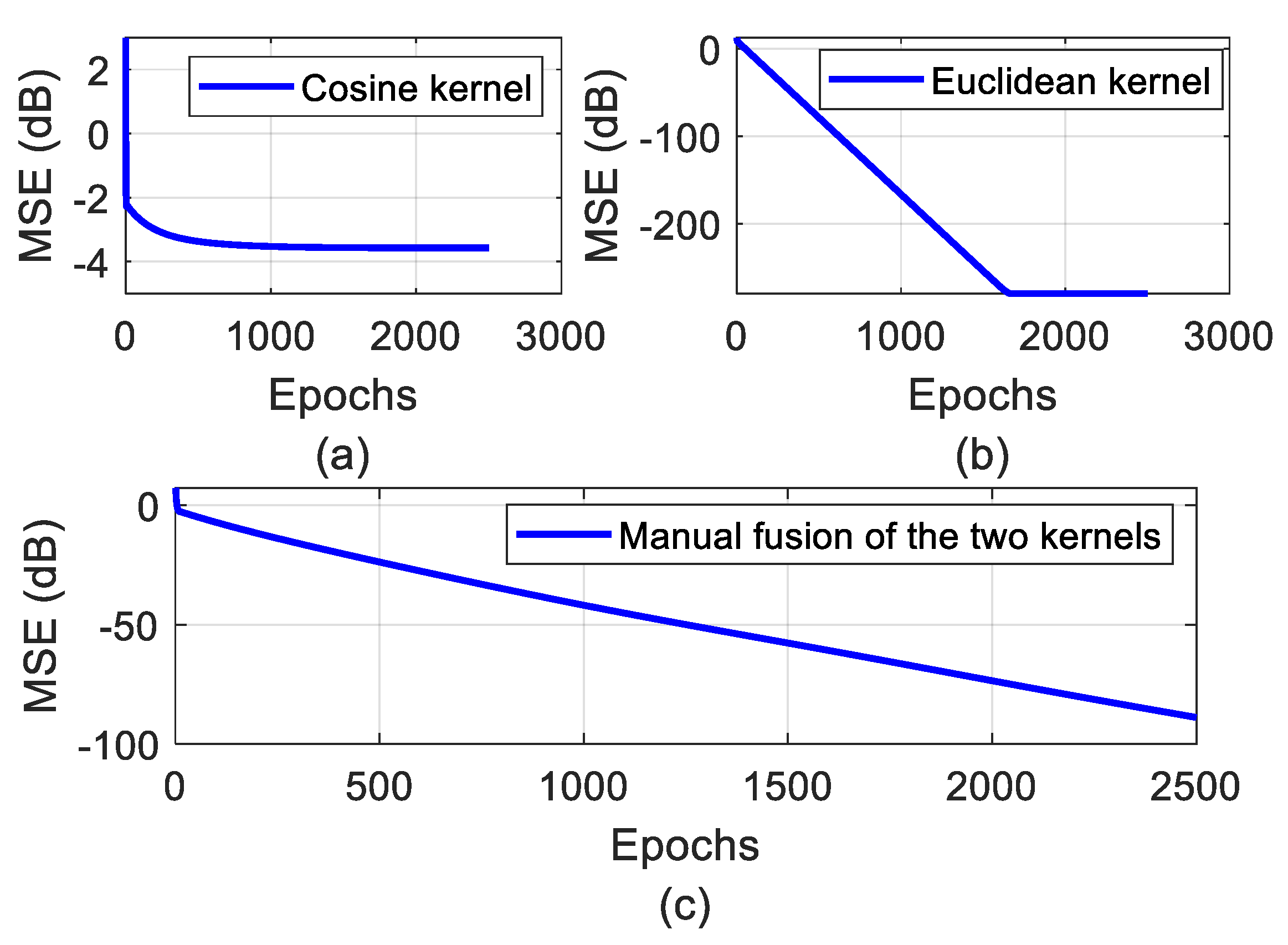
The RBFN has 14 target classes (1 normal operation and 13 faults), and the centers were chosen based on the subtractive clustering method [35,36,37] with 0.1 influence factor. Initially, the weights x i and bias b i were considered zero. The Gaussian spread is initiated at 0.2 and the value of ξ is set to be very small ( < 1 e 50 ) for the purpose of cosine kernel. The values of mixing parameters are considered 0.5 for testing the conventional kernel methods, and the corresponding results were depicted in Figure 5.
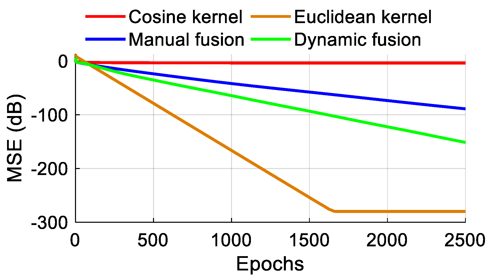
Figure 5a–c, depicts the cosine kernel RBFN, Euclidean kernel RBFN and manual fusion of kernels RBFN for the given input data and assigned parameters. It can be observed that the Euclidian kernel outperforms the cosine kernel and the manual fusion of the kernels by achieving minimum mean square error (MSE). This represented the case of overfitting, where the training performance of the system is better, but the testing performance of the system fails with the test data. These drawbacks are overcome by varying the mixing parameters of the kernel with respect to the epochs. Hence, dynamic fusion of the kernels is performed considering all the parameters mentioned previously.
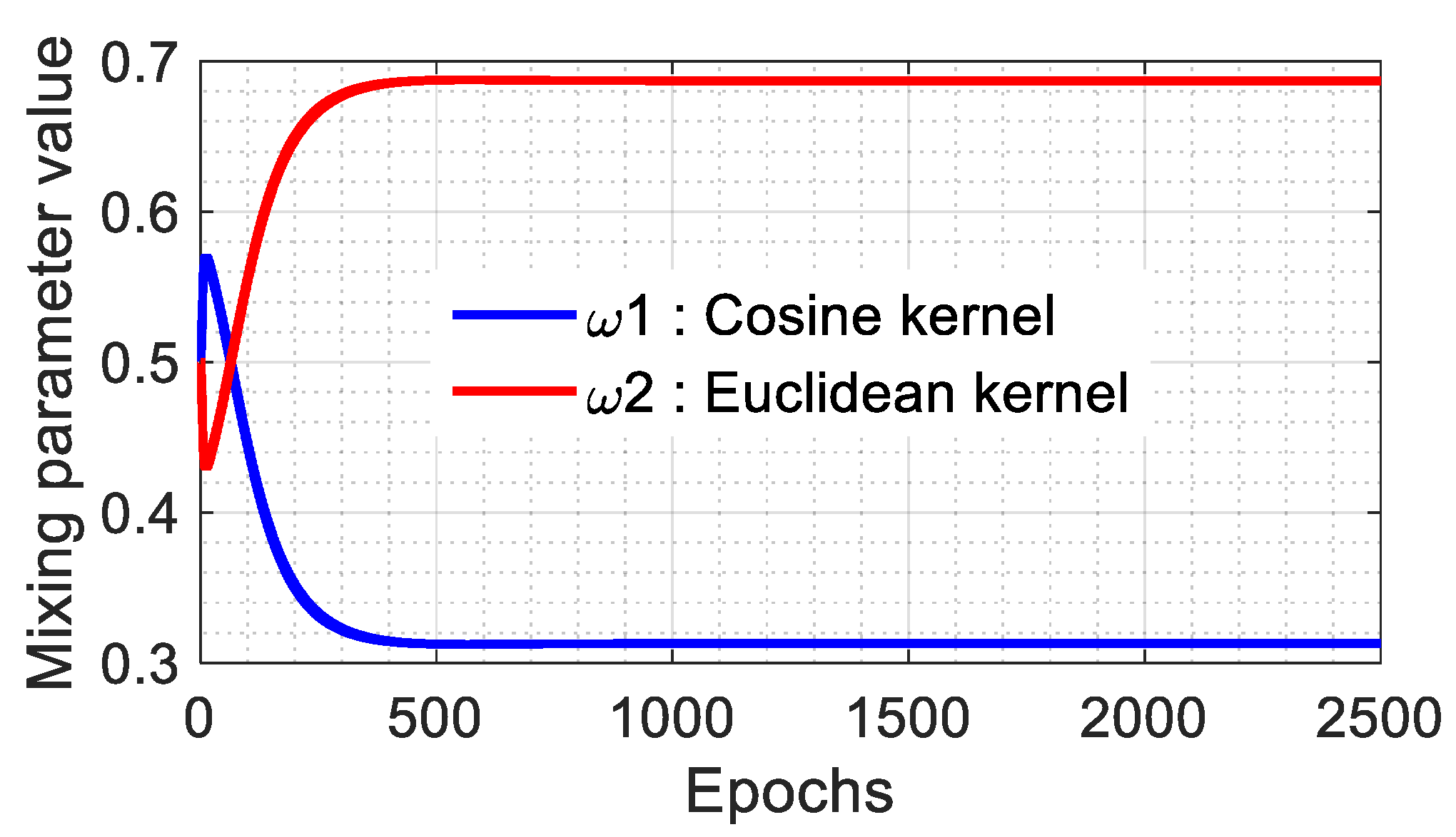
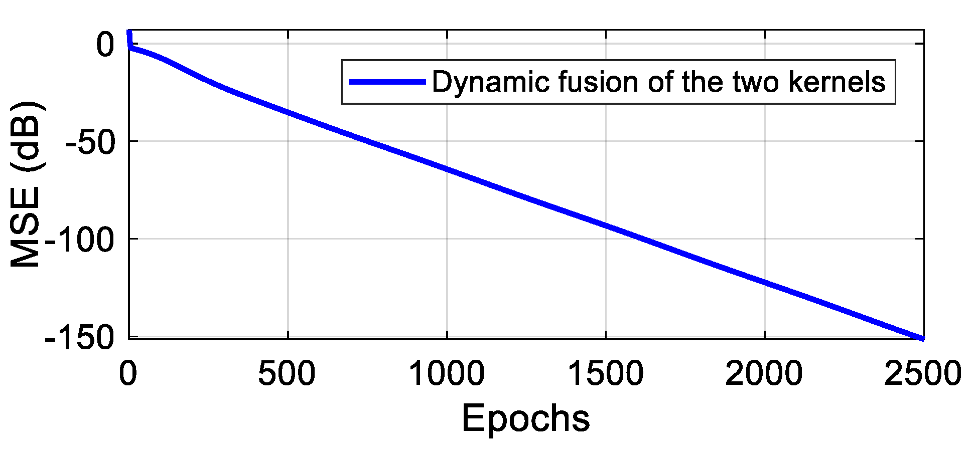
The variation of weights ω 1   &   ω 2 with respect to the number of iterations is given in Figure 6. It can be observed that after 70 epochs, there is a corresponding flip in the mixing parameters of the kernel, and further after 400 epochs, the mixing parameters become stable. Further, the mean square error curve for the dynamic fusion of cosine and Euclidean kernels to train the input data with RBFN is depicted in Figure 7. The MSE of the kernel is observed to be around −150 dB when trained for 2500 epochs which exhibited better performance than the manual fusion and cosine kernel but trailed behind the Euclidian kernel. This is explained by plotting a comparison between MSEs of all the kernels.
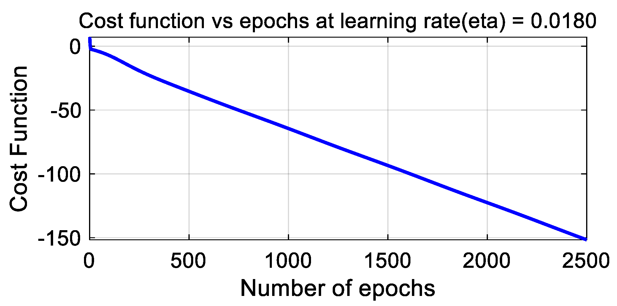
Figure 8 depicts the mean square error for all the approaches adapted for developing this algorithm. From Figure 8, it can be observed that the cosine kernel is outperformed by the Euclidean kernel by achieving a minimum mean square error of around −280 dB. It can also be observed that the mean square error of the dynamic fusion of kernels is −150 dB, which is below the Euclidean kernel error. This is due to the fact of overfitting during the training process. This condition merely provides Euclidean kernel with high training efficiency and least mean square error but fails in the phase of implementation and testing. Further, the dynamic fusion of kernel-based RBFN has a decreasing cost function or loss function, which depicts the performance of the classifier. The cost function from (22) associated with calculating the mixing parameters with a dynamic fusion of kernels is depicted in Figure 9.
The results in Table 3 support the argument of why Euclidean kernel cannot be adopted for training and testing of RBFN. Further, a comparative analysis regarding the weights assigned for every kernel and their effect on training and testing efficiency of the fault data is depicted in Table 3.

5.3. Fault Detection Results

The effectiveness of the developed fault classification algorithm was analyzed by integrating it with the PV system layout discussed in section VI A. The voltage and current measurements obtained from the system were provided as an input to the signal processing unit. The signal processing unit extracts the features of the signal in real-time and inputs them to the classification algorithm. The classification algorithm matches the input data with the trained algorithm to detect the type of fault and localize it.
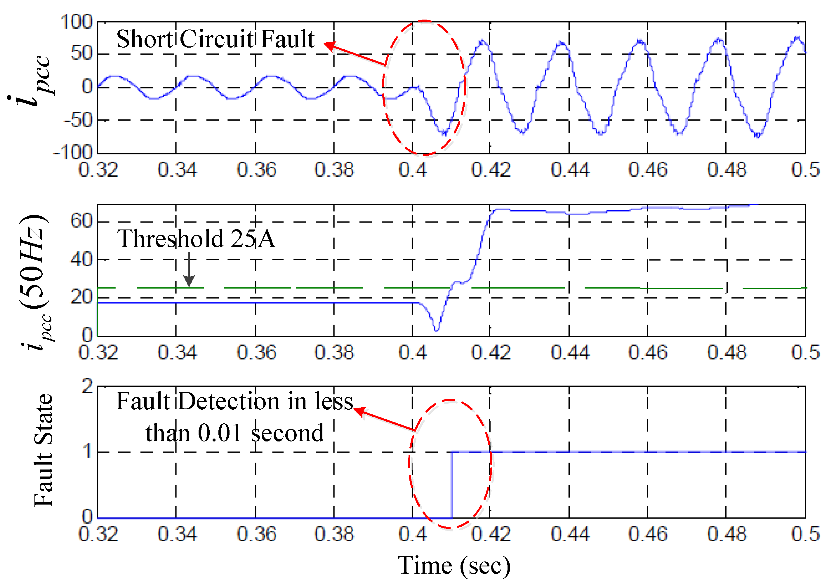
Figure 10 depicts the short circuit fault in the diode of the boost converter. The system is initially allowed to operate normally, and at t = 0.4 s, the boost converter diode is shorted. The effect of injecting short circuit fault on the boost converter diode is observed on the load current of the PV system. A threshold of 25 A for load current is set for fault detection using the trained classifier. The trained classified continuously monitors the 50 Hz component of load current i s . Once the fault is injected, the trained classifier takes 0.01   s to classify the fault.
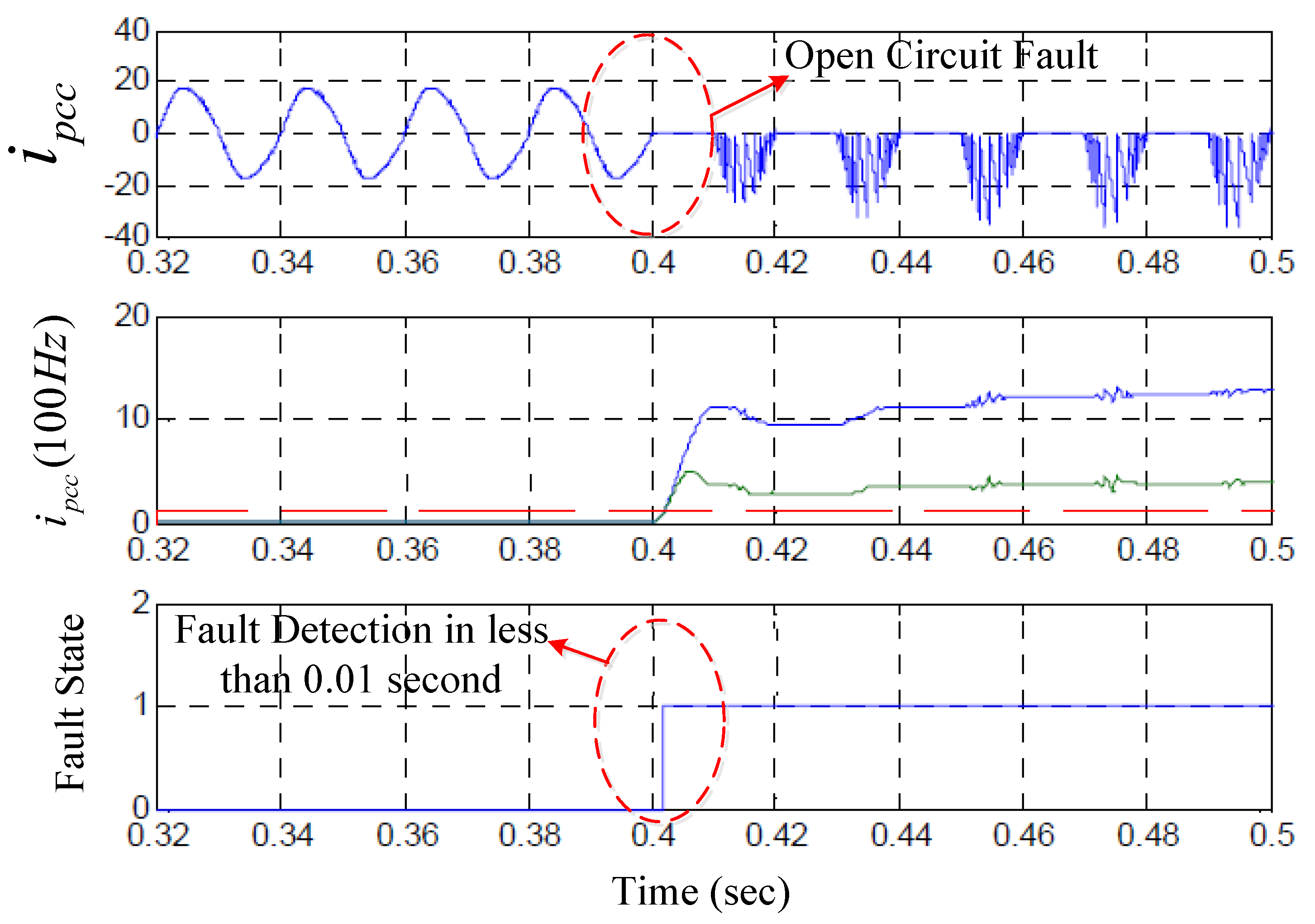
Figure 11 depicts the open circuit fault in the inverter. Initially, the system operates normally, and at t = 0.4 s, switch s1 of the inverter is opened. This creates an open circuit fault in the inverter. The effect of creating an open circuit fault is observed by continuously monitoring the load current i s . The threshold is set around 1A, and the trained classifier detected the fault in less than 0.01   s .
To test the robustness of the developed classification algorithm, different noise conditions were generated in the simulated system. The error of signal measurement sensors and environment noise were considered as additive white Gaussian noise (AWGN) in this research. In order to examine the robustness of the fault locating algorithm for different noise conditions, the fault location performance was tested with input signals containing various signal-to-noise ratio (SNR) values between 20 and 50 dB. In general, a typical SNR value of 30 dB is equivalent to a peak noise magnitude of nearly 3.5% of the voltage signal [38].
The performance of the fault locator for various PV faults in noisy conditions was analyzed in this research. However, only the results of the converter faults are discussed. Results of the fault location algorithm for converter faults using the voltage and current waveform contaminated with various levels of noise are presented in Table 4.
It is noted that although the accuracy decreases with the noise level, a satisfactory fault locating success rate can be achieved even though the input signals contain different levels of noise. Table 4 shows that overall accuracy of 97.52% could still be obtained even with a high noise level of 50 dB. Thus, it is clear that the proposed fault location algorithm has a robust performance.

6. Conclusions

This paper builds a generalized approach for fault classification of the photovoltaic system. The developed methodology performs feature extraction utilizing a wavelet-based approach and classification using an RBFN classifier. Further, the classifier is enhanced by performing manual fusion between the distinctive properties of cosine and Euclidean kernels for RBFN, which depicted a significant improvement when compared to the conventional kernels. During the manual fusion process, the weights are arbitrarily assigned using the trial and error method without any prior information about the system. Further, the problem with the manual fusion of these kernels is overcome by developing a new framework to optimize the weights. The developed approach depicted training efficiency of 100% and testing efficiency of 97.05%, which is better than conventional methods. At this level, the trained classifier is tested with short circuit and open circuit faults, which depicted a very less detection time. In order to check the real-time performance of the developed algorithm, a single-phase standalone PV system along with additive white Gaussian noise is considered. The experimental results depicted an overall accuracy of 97.52%, even with a high noise level of 50 dB.

Author Contributions

Conceptualization, methodology, software, validation, and formal analysis—V.S.B.K. and M.A.K.; Investigation—V.S.B.K. and M.A.K.; Resources, and data curation—V.S.B.K., M.A.K. and A.H.; writing—original draft preparation, writing—review and editing, and visualization—V.S.B.K. and M.A.K.; supervision—A.H. and F.B.; project administration—A.H. and F.B. All authors have read and agreed to the published version of the manuscript.

Funding

This research received no external funding.

Conflicts of Interest

The authors declare no conflict of interest.

References

  1. Parida, B.; Iniyan, S.; Goic, R. A review of solar photovoltaic technologies. Renew. Sustain. Energy Rev. 2011, 94, 779–791. [Google Scholar] [CrossRef]
  2. Shahsavari, A.; Akbari, M. Potential of solar energy in developing countries for reducing energy-related emissions. Renew. Sustain. Energy Rev. 2018, 90, 275–291. [Google Scholar] [CrossRef]
  3. Dumnic, B.; Liivik, E.; Milicevic, D.; Popadic, B.; Katic, V.; Blaabjerg, F. Fault Analysis and Field Experiences of Central Inverter Based 2 MW PV Plant. In Proceedings of the 2018 20th European Conference on Power Electronics and Applications (EPE’18 ECCE Europe), Riga, Latvia, 17 September 2018; pp. 1–10. [Google Scholar]
  4. Kurukuru, V.S.B.; Haque, A.; Khan, M.A. Fault Detection in Single-Phase Inverters Using Wavelet Transform-Based Feature Extraction and Classification Techniques. In Applications of Computing, Automation and Wireless Systems in Electrical Engineering; Springer: Singapore, 2019; pp. 649–661. [Google Scholar]
  5. Haque, A.; Bharath, K.V.S.; Khan, M.A.; Khan, I.; Jaffery, Z.A. Fault diagnosis of Photovoltaic Modules. Energy Sci. Eng. 2019. [Google Scholar] [CrossRef] [Green Version]
  6. Kurukuru, V.S.B.; Haque, A.; Khan, M.A.; Tripathy, A.K. Fault classification for Photovoltaic Modules Using Thermography and Machine Learning Techniques. In Proceedings of the 2019 International Conference on Computer and Information Sciences (ICCIS), Aljouf, Saudi Arabia, 3 April 2019; pp. 1–6. [Google Scholar]
  7. Ahmad, S.; Hasan, N.; Kurukuru, V.S.B.; Khan, M.A.; Haque, A. Fault Classification for Single Phase Photovoltaic Systems using Machine Learning Techniques. In Proceedings of the 2018 8th IEEE India International Conference on Power Electronics (IICPE), Jaipur, India, 13–15 December 2018; pp. 1–6. [Google Scholar]
  8. Zhao, Y.; De Palma, J.F.; Mosesian, J.; Lyons, R.; Lehman, B.; Zhao, Y.; De Palma, J.F.; Mosesian, J.; Lyons, R.; Lehman, B. Line–line fault analysis and protection challenges in solar photovoltaic arrays. IEEE Trans. Ind. Electron. 2013, 60, 3784–3795. [Google Scholar] [CrossRef]
  9. Nasrin, R.; Hasanuzzaman, M.; Rahim, N.A. Effect of high irradiation on photovoltaic power and energy. Int. J. Energy Res. 2018, 42, 1115–1131. [Google Scholar] [CrossRef]
  10. Hu, Y.; Zhang, J.; Cao, W.; Wu, J.; Tian, G.Y.; Finney, S.J.; Kirtley, J.L. Online Two-Section PV Array Fault Diagnosis with Optimized Voltage Sensor Locations. IEEE Trans. Ind. Electron. 2015, 62, 7237–7246. [Google Scholar] [CrossRef] [Green Version]
  11. Fatama, A.Z.; Haque, A.; Khan, M.A. A Multi Feature Based Islanding Classification Technique for Distributed Generation Systems. In Proceedings of the 2019 International Conference on Machine Learning, Big Data, Cloud and Parallel Computing (COMITCon), Faridabad, India, 14 Feberary 2019; pp. 160–166. [Google Scholar]
  12. Chen, K.Y.; Chen, L.S.; Chen, M.C.; Lee, C.L. Using SVM based method for equipment fault detection in a thermal power plant. Comput. Ind. 2011, 62, 42–50. [Google Scholar] [CrossRef]
  13. Morente-Molinera, J.A.; Mezei, J.; Carlsson, C.; Herrera-Viedma, E. Improving Supervised Learning Classification Methods Using Multigranular Linguistic Modeling and Fuzzy Entropy. IEEE Trans. Fuzzy Syst. 2017, 25, 1078–1089. [Google Scholar] [CrossRef]
  14. Zhao, Y.; Ball, R.; Mosesian, J.; de Palma, J.F.; Lehman, B. Graph-Based Semi-supervised Learning for Fault Detection and Classification in Solar Photovoltaic Arrays. IEEE Trans. Power Electron. 2014, 30, 2848–2858. [Google Scholar] [CrossRef]
  15. Li, L.; Ding, S.X.; Yang, Y.; Peng, K.; Qiu, J. A fault detection approach for nonlinear systems based on data-driven realizations of fuzzy kernel representations. IEEE Trans. Fuzzy Syst. 2018, 26, 1800–1812. [Google Scholar] [CrossRef]
  16. Aftab, W.; Moinuddin, M.; Shaikh, M.S. A novel kernel for RBF based neural networks. Abstr. Appl. Anal. 2014, 2014, 176253. [Google Scholar] [CrossRef]
  17. Tchakoua, P.; Wamkeue, R.; Ouhrouche, M.; Slaoui-Hasnaoui, F.; Tameghe, T.; Ekemb, G. Wind turbine condition monitoring: State-of-the-art review, new trends, and future challenges. Energies 2014, 7, 2595–2630. [Google Scholar] [CrossRef] [Green Version]
  18. Jordan, D.C.; Silverman, T.J.; Sekulic, B.; Kurtz, S.R. PV degradation curves: Non-linearities and failure modes. Prog. Photovolt. Res. Appl. 2017, 25, 583–591. [Google Scholar] [CrossRef] [Green Version]
  19. King, D.L.; Boyson, W.E.; Kratochvil, J.A. Analysis of factors influencing the annual energy production of photovoltaic systems. In Proceedings of the Conference Record of the Twenty-Ninth IEEE Photovoltaic Specialists Conference, New Orleans, LA, USA, 19–24 May 2002; pp. 1356–1361. [Google Scholar]
  20. Petrone, G.; Spagnuolo, G.; Teodorescu, R.; Veerachary, M.; Vitelli, M. Reliability Issues in Photovoltaic Power Processing Systems. IEEE Trans. Ind. Electron. 2008, 55, 2569–2580. [Google Scholar] [CrossRef]
  21. Khan, M.A.; Haque, A.; Kurukuru, V.S.B. An Efficient Islanding Classification Technique for Single Phase Grid Connected Photovoltaic System. In Proceedings of the 2019 International Conference on Computer and Information Sciences (ICCIS), Aljouf, Saudi Arabia, 3–4 April 2019; pp. 1–6. [Google Scholar]
  22. He, J.; Yu, B. Continuous wavelet transforms on the space L2 (R, H; dx). Appl. Math. Lett. 2004, 17, 111–121. [Google Scholar] [CrossRef] [Green Version]
  23. Mallat, S. A Wavelet Tour of Signal Processing, 3rd ed.; The Sparse Way; Academic Press: Cambridge, MA, USA, 2008. [Google Scholar]
  24. Stéphane, M. Time Meets Frequency. In A Wavelet Tour of Signal Processing; Elsevier: Amsterdam, The Netherlands, 2009; pp. 89–153. [Google Scholar]
  25. Han, M.; Guo, W.; Mu, Y. A modified RBF neural network in pattern recognition. In Proceedings of the 2007 International Joint Conference on Neural Networks, Orlando, FL, USA, 12–17 August 2007; pp. 2527–2532. [Google Scholar]
  26. Wang, W.; Xu, Z.; Lu, W.; Zhang, X. Determination of the spread parameter in the Gaussian kernel for classification and regression. Neurocomputing 2003, 55, 643–663. [Google Scholar] [CrossRef]
  27. Mai-Duy, N.; Tran-Cong, T. Numerical solution of Navier-Stokes equations using multiquadric radial basis function networks. Int. J. Numer. Methods Fluids 2001, 37, 65–86. [Google Scholar] [CrossRef]
  28. Mongillo, M. Choosing Basis Functions and Shape Parameters for Radial Basis Function Methods. SIAM Undergrad. Res. Online 2011, 4, 190–209. [Google Scholar] [CrossRef]
  29. Danielsson, P.E. Euclidean distance mapping. Comput. Graph. Image Process. 1980, 14, 227–248. [Google Scholar] [CrossRef] [Green Version]
  30. Meza, J.C. Steepest descent. Wiley Interdiscip. Rev. Comput. Stat. 2010, 2, 719–722. [Google Scholar] [CrossRef]
  31. Khan, M.A.; Haque, A.; Kurukuru, V.S.B. Performance Assessment of Stand-Alone Transformerless Inverters. 2020. Available online: https://onlinelibrary.wiley.com/doi/abs/10.1002/2050-7038.12156 (accessed on 7 January 2020).
  32. Khan, M.A.; Haque, A.; Kurukuru, V.S.B. Control and Stability Analysis of H5 Transformerless Inverter Topology. In Proceedings of the 2018 International Conference on Computing, Power and Communication Technologies (GUCON), Greater Noida, India, 28–29 September 2018; pp. 310–315. [Google Scholar]
  33. Khan, M.A.; Haque, A.; Kurukuru, V.S.B. Hybrid Voltage Control for Stand Alone Transformerless Inverter. In Proceedings of the IEEE International Conference on Power Electronics, Intelligent Control and Energy 2018 (ICPEICES), New Delhi, India, 22–24 October 2018. [Google Scholar]
  34. Daubechies, I. Ten Lectures of Wavelets; Springer: Berlin/Heidelberg, Germany, 1992; p. 357. [Google Scholar]
  35. Kim, D.W.; Lee, K.; Lee, D.; Lee, K.H. A kernel-based subtractive clustering method. Pattern Recognit. Lett. 2005, 26, 879–891. [Google Scholar] [CrossRef]
  36. Sarimveis, H.; Alexandridis, A.; Bafas, G. A fast training algorithm for RBF networks based on subtractive clustering. Neurocomputing 2003, 51, 501–505. [Google Scholar] [CrossRef]
  37. Yang, P.; Zhu, Q.; Zhong, X. Subtractive clustering based RBF neural network model for outlier detection. J. Comput. 2009, 4, 755–762. [Google Scholar] [CrossRef]
  38. Uyar, M.; Yildirim, S.; Gencoglu, M.T. An effective wavelet-based feature extraction method for classification of power quality disturbance signals. Electr. Power Syst. Res. 2008, 78, 1747–1755. [Google Scholar] [CrossRef]
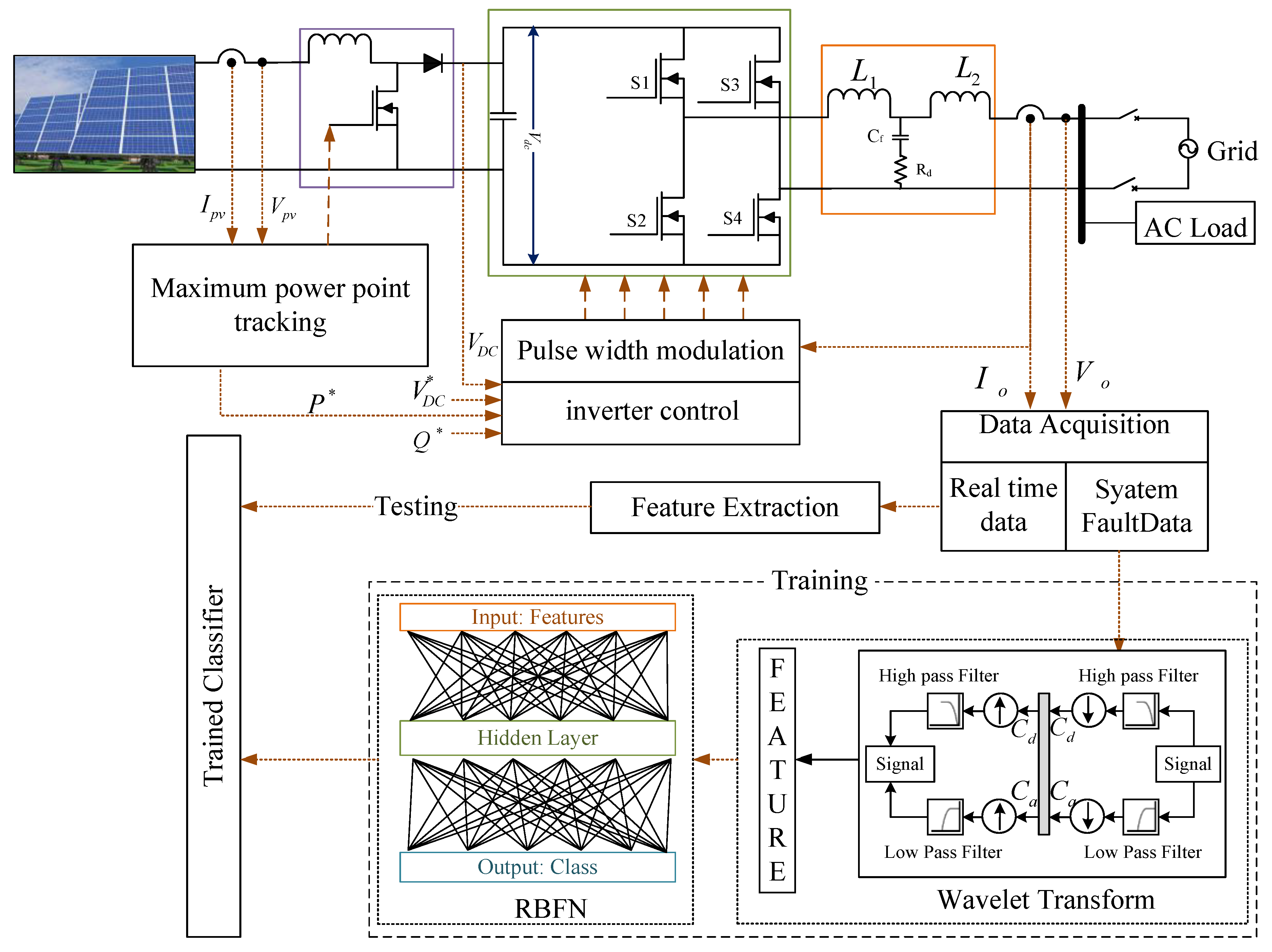
Figure 1. Proposed fault classification process is standalone PV system.
Energies 13 00308 g001
Figure 2. Faults in a photovoltaic system.
Energies 13 00308 g002
Figure 3. Structure of the Radial Basis Function Neural Network.
Energies 13 00308 g003
Figure 4. Faults simulated in the single-phase two-stage standalone PV system.
Energies 13 00308 g004
Figure 5. Mean Square Error curves of the training phase (a) Cosine Kernel, (b) Euclidean Kernel, (c) Manual fusion of Cosine and Euclidean Kernel.
Energies 13 00308 g005
Figure 6. Mixing parameters for dynamic fusion of kernels.
Energies 13 00308 g006
Figure 7. Mean square error curve of the training phase of the dynamic fusion of kernels.
Energies 13 00308 g007
Figure 8. Comparison of mean square error curves of the training phase of the different kernels for pattern recognition.
Energies 13 00308 g008
Figure 9. Cost function vs. eta (Epochs at learning rate) for mixing parameters.
Energies 13 00308 g009
Figure 10. Boost converter diode short circuit fault.
Energies 13 00308 g010
Figure 11. Inverter switch open circuit fault.
Energies 13 00308 g011
Table 1. Fault Mode and their potential causes and effects.
Fault TypePotential CausePotential Effect
Module Failure (loss of electrical function)Open contacts, Short circuit and arcingNo energy output
Impairment of electric functionHigh series resistance, low shunt resistance, aging, shading, soilingReduced energy output, hot spot damage
Junction box/bypass diode open contactsDisconnections, improper installation, corrosion,No energy output
Short, arc in contactsDamaged insulation, aging, and lightning.No energy output, thermal damages, fire
Inverter fails to transferContact damage, excessive heating of switches, software failure with gating pulsesDistorted or No energy output
Degraded outputMPPT unbalance, Extreme weather conditionsReduced energy output
Spurious tripBad system configuration, corrosion, aging, lack of maintenanceNo energy output
Table 2. Faults analyzed in the simulated PV system.
ComponentOperating ConditionDescription
PV System (1 kW)Normal Operation (N. O)Operated under standard test conditions.
PV ModulePartial Shading (Fault 1)Low power output from the modules
cell bypass (Fault 2)Low power output from the modules
PV ArrayLine to Line Fault (Fault 3)Negative current from the faulted string (back-fed current)
Ground Faults (Fault 4)Undesirable condition of current flowing through the equipment grounding conductor in the circuits carrying DC power
Boost converterInductance open circuit (Fault 5)Inductor is disconnected from the boost converter circuit resulting in a maximum DC component of the VI (voltage current characteristic) curve.
DC link capacitance open (Fault 6)The positive point of the DC link capacitor is disconnected, which results in a highly abnormal DC component.
Diode open (Fault 7)One terminal of boost converter diode is disconnected, which results in a nullified frequency of the component.
Diode short circuit (Fault 8)Boost converter diode is short-circuited by using a cable, which results in a change of voltage magnitude.
Switch open (Fault 9)The MOSFET is disconnected or open-circuited due to bond wire lift off, resulting in a nullified frequency of the component.
Switch short circuit (Fault 10)The MOSFET is shorted, which results in the minimum DC component of the IV curve.
Switches (s1, s2, s3, and s4) open (Fault 11)The switches of inverter were disconnected one at a time along with the diode, and the corresponding effects were observed.
InverterSwitches (s1, s2, s3, and s4) short circuit (Fault 12)The power switches and diode of inverter were short-circuited one at a time, and the corresponding effects were observed.
Combination of open and short-circuit switches (Fault 13)Open and short circuit combinations of switches in both the converter circuits were tested, and the corresponding system operation is observed.
Table 3. Results of the training and testing process for different kernels.
Kernel TypeTraining ProcessTesting Process ω 1 ω 2
Cosine100%94.11%0.570.429
Gaussian Euclidian100%58.82%0.5730.426
Manual Fusion100%94.16%0.50.5
Dynamic Fusion100%97.05%0.5760.426
Table 4. Testing efficiency for various faults under different noise ratios.
Fault LocationTesting Efficiency
20 dB30 dB40 dB50 dB
No Fault100%98.84%97.61%97.59%
Boost ConverterFault 198.72%98.68%97.28%97.52%
Fault 298.63%96.23%98.39%98.25%
InverterFault 199.16%96.35%97.28%96.94%
Fault 296.44%97.22%96.47%97.34%