Comparative Risk Assessment for Fossil Energy Chains Using Bayesian Model Averaging ^†

Abstract

The accident risk of severe (≥5 fatalities) accidents in fossil energy chains (Coal, Oil and Natural Gas) is analyzed. The full chain risk is assessed for Organization for Economic Co-operation and Development (OECD), 28 Member States of the European Union (EU28) and non-OECD countries. Furthermore, for Coal, Chinese data are analysed separately for three different periods, i.e., 1994–1999, 2000–2008 and 2009–2016, due to different data sources, and highly incomplete data prior to 1994. A Bayesian Model Averaging (BMA) is applied to investigate the risk and associated uncertainties of a comprehensive accident data set from the Paul Scherrer Institute’s ENergy-related Severe Accident Database (ENSAD). By means of BMA, frequency and severity distributions were established, and a final posterior distribution including model uncertainty is constructed by a weighted combination of the different models. The proposed approach, by dealing with lack of data and lack of knowledge, allows for a general reduction of the uncertainty in the calculated risk indicators, which is beneficial for informed decision-making strategies under uncertainty.

1. Introduction

In the present-day world, the energy sector, including its associated infrastructure, is considered critical since it is the foundation for commodities and services. Since the 2000s, accidents in the energy sector have become a strong concern by policy makers and the general public for two main reasons. First, a number of unusally disastrous events occurred with correspondingly high media coverage (e.g., the gas well explosion in Chongqing, China in 2003, the Deep-Water Horizon Oil Spill in 2010, the Fukushima Nuclear Disaster in 2011, the Amuay refinery accident in 2012, the Soma coal mine accident in 2014, etc.). Second, accident risks have become recognized as an important aspect to evaluate the safety, security and sustainability of energy technologies, as well as in the context of critical infrastructure protection, resilience and policy formulation by decision makers [1,2,3,4]. Therefore, a comprehensive assessment of accident risks and their potential consequences is of great relevance for highly industrialized countries as well as emerging economies and developing countries [5].

The most common approach to analyze the risk of accidents in the energy sector relies on quantitative measures such as aggregated risk indicators (e.g., fatality rates) [6,7,8], allowing to compare energy chains in a comparative and comprehensive manner [6]. In this context, the calculation of objective risk indicators comprises a valuable element to support decision makers in the assessment of current and future technology portfolios [9]. Hence, there is a clear need for more and better data, and accordingly, improved uncertainty quantification for accident risk indicators, because they are the basis to support decision-makers and risk managers in their efforts to design and implement better risk management strategies, risk mitigation and prevention measures processes [10,11,12]. More recently, resilience-driven strategies have been proposed for environmental systems (e.g., marine ecosystems) that are synergistically based on risk assessment to appropriately protect against uncertain and unexpected events such as, for example, oil spills [13]. In the past years, numerous overviews and summaries about conceptual and methodologial treatments of uncertainty within risk assessment have been published [14,15,16,17,18,19]. This is related to the increasing interest in uncertainty estimation, which is of great importance to consider possible random fluctuations, i.e., caused by lack of data. In fact, as the number of historical observations decreases, the uncertainty increases. This is mainly shown for extreme accidents, where few events are commonly observed.

In the context of accident risk in the energy sector, only recently activities related to the treatment of uncertainties in a consistent way have been developed. In particular, in [20], credibility intervals (e.g., 5–95%) were firstly constructed for point estimates using a Chi-square distribution [21]; however, without considering that the uncertainty is a combination, among others, of epistemic and aleatory factors [22]. In order to consider a more complex uncertainty assessment, [13,23,24,25] analysed the risk of accidents in different energy chains chains using a Bayesian inference. In this way, the authors could estimate the risk indicators and their uncertainties, since the latter is intrinsically assessed through a Bayesian approach. In fact, a Bayesian data analysis is a fully probabilistic approach, since it accounts for both epistemic and aleatory uncertainties. The posterior distribution in a Bayesian analysis is given by the product of an a priori distribution, which defines the lack of knowledge (epistemic uncertainty), and a likelihood function, which describes the randomness of the data (aleatory uncertainty) [26]. Generally, the likelihood function is specified by experts or through the scientific community agreement [27]. Therefore, the likelihood function could be affected by both aleatory and epistemic, due to subjectivity involved in its choice, uncertainties.

Based on these premises, Bayesian Model Averaging (BMA) has been proposed in order to take into account for model uncertainty by considering a set of possible models that could describe a dataset [28]. In BMA, the average posterior distribution is given as the sum of the products of each posterior distribution estimated for each considered model with its corresponding weight. First proposed by [29], in order to include model uncertainty in the Bayesian analysis, the interest in BMA has grown since then based on both improved computational power and technical developments [30]. In this context, BMA has been applied in different scientific disciplines, such as risk assessment [24,31,32], ecology [33], social research [34], extreme values analysis [35], climate projections [36], forecasting and prediction purposes [37,38], management purposes [39], CO₂ storage related uncertainty quantifications [40], spatial models [41], etc.

In the analysis proposed in [24], the BMA concept has only been applied to the severity distribution to assess accident risk indicators in the energy sector for the period 1970–2008. In contrast, the method has been extended and completed within the current study. In particular, the analysis covers severe (e.g., ≥5 fatalities) accidents in Coal, Oil and Natural gas. energy chains for the years 1970–2016. Historical observations have been collected from the Paul Scherrer Institute (PSI)’s ENergy-related Severe Accident Database (ENSAD), see Section 2. First, based on the definition of risk as product of frequency and severity, the BMA method is applied to both of these risk parameters used in the assessment. Similar to [24], for the severity distribution model the BMA is applied to a set of models commonly used in hazard, risk assessment and survival analysis [42,43]. Furthermore, for the frequency model in this study, the BMA is applied to a group of counting models, which are commonly used to simulate discrete distributions [42,44,45] (Section 3). Therefore, in contrast to [24], results are presented here for both frequency and severity distributions in which aleatory and epistemic uncertainties are considered. Subsequently, BMA frequency and severity results are combined in a comparative risk assessment framework similar to [20] for different energy chains and country groups (Organization for Economic Co-operation and Development (OECD), non-OECD, 28 Member States of the European Union (EU28)). Finally, the results are compared to the risk calculated using an empirical approach, where the arithmetical average of fatalities and its related frequency are estimated (Section 4). This is used to validate the usefulness of the proposed method for accident risk assessment in the energy sector.

2. Data

2.1. ENSAD

The ENergy-related Severe Accident Database (ENSAD) collects accidents in the energy sector that occurred in various energy chains since 1970, taking a worldwide and full-chain perspective [46,47,48]. In ENSAD, data on all energy-related accidents is collected and classified into energy chains, e.g., Coal (including Lignite), Oil and Natural Gas, and activities within those chains. In general, an energy chain may comprise the following stages: exploration, extraction, processing, storage, transportation, power and/or heat generation, waste treatment and disposal. However, not all these stages are relevant for a specific energy chain [48]. In addition, other type of information, such as georeferenced location, types of consequences (e.g., human health, environmental and economic impacts), etc., are coded in ENSAD to achieve a comprehensive global coverage of severe accidents [48]. ENSAD has been developed using proprieatory (commercial) and publicly available (non-commercial) primary information sources, such as industrial databases, technical reports, journal and newspaper articles, websites, etc., ENSAD focuses on severe accidents since industries, stakeholders, decision-makers, etc., are more concerned about them, although small accidents have been collected for specific projects [49]. In ENSAD, seven consequence types (e.g., ≥5 fatalities, ≥10 injuries, etc.) are taken into account, and an accident is considered to be severe if it meets the threshold value for at least one of them [48]. Although different types of consequences are collected in ENSAD, in this study, particular attention has been given to fatalities in fossil energy chains for the period 1970–2016. Fatalities have been chosen, since they generally comprise the most reliable consequence indicator with regard to completeness and accuracy of the data [5].

2.2. Country Groups

Comparative results can be provided at different levels, from individual countries to different country groups [8,20]. However, the feasible level of resolution is normally determined by the amount of available data in a given study. Therefore, often the intermediate level of country groups is chosen because it allows differentiation between well defined entitites [20]. In this study, three major country groups, namely OECD, non-OECD and EU28, have been selected due to their differences in regulatory frameworks and safety culture. Similar to [20], as a first approximation, for all the considered country groups accidents have been allocated to each of them considering the present time member states, i.e., avoiding temporal variation in membership. Furthermore, Coal China have been separated from Coal non-OECD since it has been shown that data before 1994 are affected by significant underreporting [50]. Furthermore, Chinese coal data were separated in three time periods for 1994–1999, 2000–2008 and 2009–2016, because data of the first period is based on official Chinese data [50], the second one uses freely available Chinese information sources and the third one is principally based on news reports.

Table 1. Total numbers of severe (≥5 fatalities) accidents and their respective fatalities for selected energy chain and country group combinations in the years 1970–2016.

Energy Chain	Country Group	Number of Accidents	Number of Fatalities
Coal	OECD	110	2927
	non-OECD w/o China	222	6143
	EU28	50	1360
	China 1994–1999	817	11,059
	China 2000–2008	1182	14,662
	China 2009–2016	275	2435
Oil	OECD	199	3780
	non-OECD	494	17,832
	EU28	167	1186
Natural Gas	OECD	124	1420
	non-OECD	123	2127
	EU28	41	411

summarizes the severe accidents considered in this study.

2.3. Frequency and Fatality Distributions

Risk can be defined in different way, depending on the specific aim and the topic of the analysis [51]. In this study, risk is defined as the product of the frequency and the severity, as commonly used in natural sciences and engineering [20]. The frequency is defined by the number of accidents per year, while the severity indicates the consequence magnitude of an accident, which in this study is described by the number of fatalities, see Section 2.1. Frequency and fatality distributions for each energy chain show different statistical behaviour (Figures S1–S6 in the Supplementary Material). The frequency distribution (Figures S1–S3) is influenced by technological and regulatory differences and changes within each chain as well as country groups. On the other hand, the fatality distribution stretches over a broad range as shown in Figures S4–S6. In all cases, the distributions are right-skewed (skewness > 0), meaning that most of the accidents are located at the left side of the mean, with catastrophic (extreme) events located to the right of the distribution.

2.4. Normalization

The normalization factor, in terms of unit of energy produced, is used to obtain a comparable risk measure across energy chains and country groups. In this study, risk is normalized by the average production per year for each energy chain and country group in The Gigawatt-electric-year (GWeyr) (

Table 2. Overview of the total and average annual production (GWeyr) for the analyzed energy chains and country groups for the years 1970–2016 [52]. In this study, the average annual production is used for normalization pourposes.

Energy Chain	Country Group	Total Production (GWeyr)	Average Annual Production (GWeyr)
Coal	OECD	21,853	465
	non-OECD w/o China	19,377	412
	EU28	6799	145
	China 1994–1999	1877	313
	China 2000–2008	4559	507
	China 2009–2016	6600	825
Oil	OECD	19,383	412
	non-OECD	53,968	1148
	EU28	2488	53
Natural Gas	OECD	17,707	377
	non-OECD	22,220	473
	EU28	3667	78

). The GWeyr is a common unit to use for normalized indicators in technology assessment. It is estimated starting from the energy produced in Mtoe (Milion tons of oil equivalent) collected in [52] and by considering a generic efficiency factor of 0.35 [46] to convert from thermal energy to its electrical output equicalent as follows:

$$\mathrm{GWeyr}=\frac{\mathrm{Mtoe}\times 11630}{24\times 365}\times 0.35=\frac{\mathrm{GWh}}{24\times 365}\times 0.35$$

(1)

Furthermore, the average annual production has been chosen, since results for the risk are provided in terms of expected (average) frequency and fatalities.

3. Method

The Bayesian Model Averaging (BMA) is an extension of the classical Bayesian analysis. In the latter, the posterior distribution $p(\theta | y)$ for a parameter of interest (e.g., expected fatalities) is commonly sampled through Markov Chain Monte-Carlo (MCMC) method from the product of an a priori distribution $p\left(\theta \right)$, which describes what is known before observing the data, and the likelihood function (model) representing the data $L\left(y;\theta \right)$ [53]:

$$p(\theta |y)\propto L\left(y;\theta \right)p\left(\theta \right)$$

(2)

Therefore, Bayesian analysis is a fully probabilistic approach, since it considers both epistemic (through the prior distribution) and aleatory (through the model) uncertainties. However, inference based on a single model does not consider model uncertainty related to the subjective choice of the likelihood function. In this context, to reduce these uncertainties BMA is applied [28,30].

In BMA, the posterior distribution of a parameter of interest is derived over some space of possible models instead of only one. Let us consider M as a set of potential models of interest M_j, with $M_j \in M$. If θ is the parameter of interest, and the likelihood corresponding to the model M_j is given by $L\left(y;\theta , M_j\right)$, then Equation (2) can be rewritten as:

$$p(\theta |y)\propto \sum _{j=1}^{J}p(\theta |y,M_j)p(M_j|y)$$

(3)

This is the weighted average of the posterior distribution under each model M_j, where the weights are determined by the posterior model probabilities $p \left(M_j\right| y)$. Furthermore, the posterior density under M_j can be rewritten as [40]:

$$p(\theta |y,M_j)\propto L\left(y;\theta ,M_j\right)p(\theta |M_j)$$

(4)

This is similar to Equation (2), where $p(\theta | M_j)$ is the a priori distribution under M_j, which in this study is modeled as non-informative due to the lack of knowledge [24], and $L\left(y; \theta , M_j\right)$ is the likelihood function. Similar to Equation (2), this posterior distribution can be estimated by using a sampling approach, i.e., MCMC algorithms [38]. On the other hand, in Equation (3), the posterior probability for model M_j is given by [28]:

$$p(M_j|y)=\frac{m(y|M_j)p\left(M_j\right)}{{\sum }_{i=1}^{J}m(y|M_i)p\left(M_i\right)}$$

(5)

where $p\left(M_j\right)$ represents the weight of the model M_j. In this study, $p\left(M_j\right)=1/J$, with j = 1, …, J, i.e., giving equal probability to each model before the observation of the data. Furthermore, $m(y | M_j)$ is the marginal density of the observations under M_j, i.e., the probability computed integrating the likelihood multiplied by the prior distribution of the parameters over the parameter space [38]:

$$m(y | M_j)= {\int }^{}{L}_j\left({\theta }_j; y\right)p({\theta }_j| M_j)d{\theta }_j$$

(6)

This integral can be difficult to compute, because a closed form might not be always available. In fact, in BMA, the relationship between the likelihood function and the model list could be significantly different depending if the data generating the model belongs to the set of selected models (M-close), if the model exists and it is known to be out of the model list, but intractable (M-complete) or difficult to conceptualize (M-open) [54]. In this context, depending on the type of relationship between the likelihood function and the model list, in the literature different methods have been developed to compute the integral in Equation (6) or even approximate Equation (5) [30]; among them, there is the Kullback–Leibler (KL) divergence [55], the Median Probability Model [56], the Stacking method [54], the Watanabe-Akaike Information Criterion (WAIC) method [57], the Bayesian Information Criterion (BIC) method [31] and the MCMC algorithms [58].

In this study, and for both frequency and severity distributions, the model exists; however, it is not clear if it belongs to the list of selected models or not. In this context, the relationship between the likelihood function and the model list is considered as M-open, since not enough information or knowledge about the real models are given for both distributions, i.e., they are difficult to conceptualize. Therefore, one of the best methods to assess Equation (5) is the one that maximizes the expected utility with respect to the true model. This is commonly done by using the KL divergence, the WAIC or the BIC methods, since they maximize the likelihood, reducing the conceptual and computational issues related to the specification of the posterior probability for model M_j explicit form [54]. In particular, the BIC method is employed in this study, since it is adequate when non-informative priors, as considered in this study due to lack of knowledge, are assumed over the entire model space [43]. In fact, by looking at Equation (2), if the prior is non-informative, the posterior distribution can be approximated to the likelihood function as $p(\theta | y) ~ L\left(y; \theta \right)$. In a similar manner, in Equation (6), the introduction of an a priori distribution can be bypassed. Under these conditions, the posterior model weight can be described in terms of BIC as follows [58]:

$$p(M_j|y)=\frac{\exp \left(-0.5\times BI{C}_j\right)}{{\sum }_{i=1}^J\exp \left(-0.5\times BI{C}_i\right)}$$

(7)

where $BI{C}_j= -2L_j\times p_j\times logN$, with N the sample size of the training set, p is the total number of parameters and L is the log-likelihood. Moreover, the lower the BIC score the better the model fits the dataset. Therefore, as higher the BIC score as lower the weight will be given to $p(M_j | y)$.

4. Results and Discussions

The BMA method is applied to both the frequency, in terms of accidents per average annual production in GWeyr (Table 2), and severity, in terms of fatalities per accident, to subsequently estimate the accident risk in the form of aggregated indicators, i.e., fatalities per GWeyr. In other words, the accident risk is estimated in terms of mean and 5–95% quantiles of the mean by multiplying the mean and the 5–95% quantiles of the frequency by the ones of the severity. All calculations were carried out for the different fossil energy chains (Coal, Oil and Natural Gas) and country groups (OECD, non-OECD, EU28).

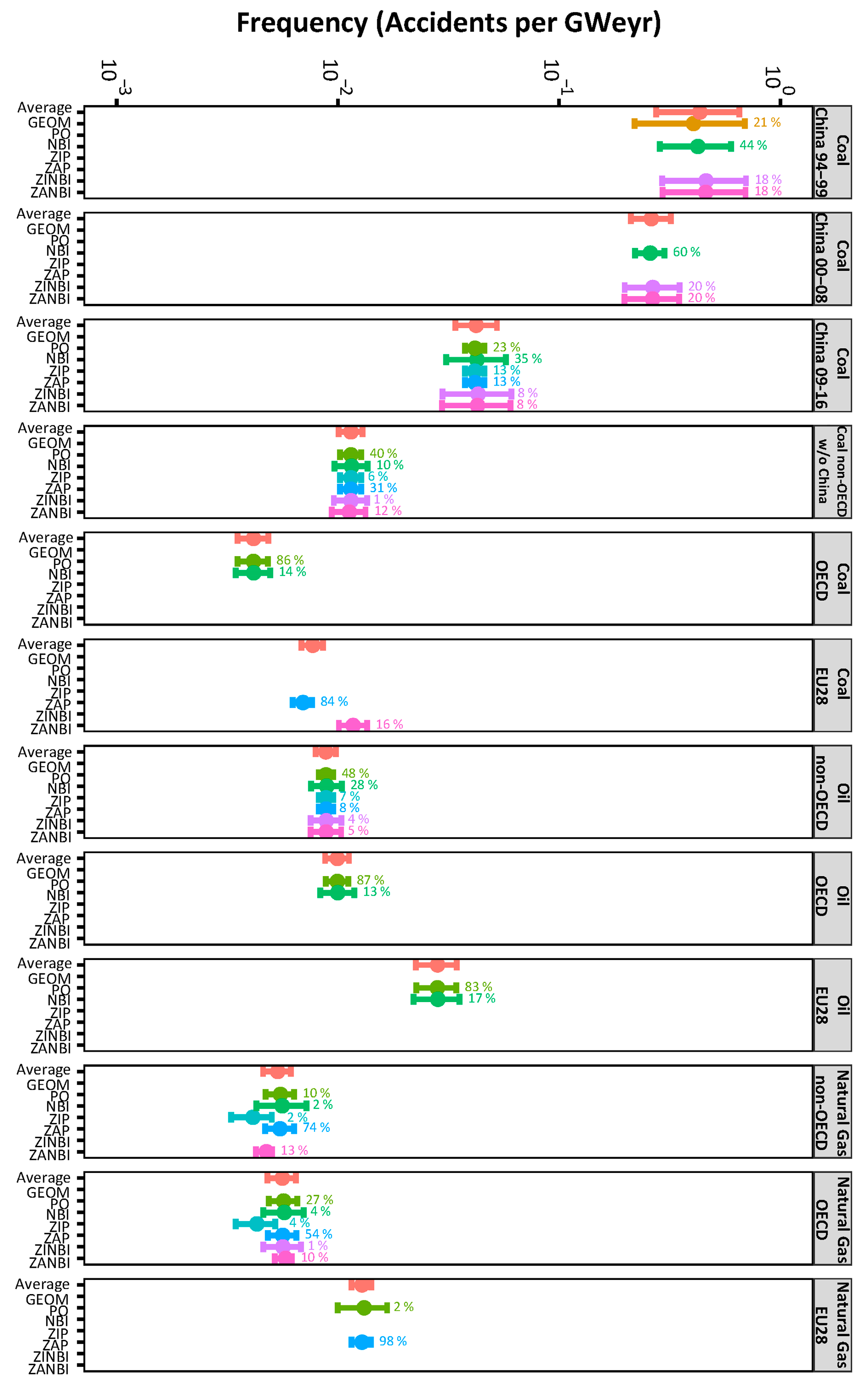
4.1. Frequency Distributions

The frequency is measured as the number of accidents per average annual production in GWeyr (Figures S1–S3). In the ENSAD database, severe accidents can be considered rare events and their behaviour as discrete in statistical terms. Based on this premise, a unique model describing the frequency is difficult to establish, which is why the BMA method is applied (Section 3). In this context, the model space for frequency is specified by a selection of counting models, which are commonly used to simulate discrete distributions [42,44,45]. The geometric (GEOM), Poisson (PO), negative binomial (NBI), zero-inflated Poisson (ZIP), zero-altered Poisson (ZAP), zero-inflated negative binomial (ZINBI) and zero-altered negative binomial (ZANBI) are the models considered in this study (

Table 3. Summary of goodness of fit (Bayesian Information Criterion (BIC) score) and relative posterior model weight (Weight) for the frequency distributions collected for different fossil energy chains and country groups. In bold the weights of each model contributing equal or more than 0.01%, and thus selected for further analysis. The green cells highlighted the different contribution of each model (the lighter the higher). GEOM = Geometric; PO = Poisson; NBI = Negative Binomial; ZIP = Zero-Inflated Poisson; ZAP = Zero-Altered Poisson; ZINBI = Zero-Inflated Negative Binomial; ZANBI = Zero-Altered Negative Binomial.

Energy Chain	Country Group	Results	Distributions
			GEOM	PO	NBI	ZIP	ZAP	ZINBI	ZANBI
Coal	China 1994–1999	BIC	74	323	73	324	324	75	75
		Weight	0.21	0.00	0.44	0.00	0.00	0.18	0.18
	China 2000–2008	BIC	110	137	94	139	139	97	97
		Weight	0.00	0.00	0.60	0.00	0.00	0.20	0.20
	China 2009–2016	BIC	75	59	58	60	60	61	61
		Weight	0.00	0.23	0.35	0.13	0.13	0.08	0.08
	non-OECD w/o China	BIC	242	207	211	212	208	214	210
		Weight	0.00	0.40	0.10	0.06	0.31	0.01	0.12
	OECD	BIC	322	266	270	620	490	630	513
		Weight	0.00	0.86	0.14	0.00	0.00	0.00	0.00
	EU28	BIC	115	88	92	92	77	95	81
		Weight	0.00	0.00	0.00	0.00	0.84	0.00	0.16
Oil	non-OECD	BIC	313	258	259	262	262	263	263
		Weight	0.00	0.48	0.28	0.07	0.08	0.04	0.05
	OECD	BIC	386	312	315	473	572	501	590
		Weight	0.00	0.87	0.13	0.00	0.00	0.00	0.00
	EU28	BIC	178	147	150	254	310	366	371
		Weight	0.00	0.83	0.17	0.00	0.00	0.00	0.00
Natural Gas	non-OECD	BIC	164	131	134	134	127	138	130
		Weight	0.00	0.10	0.02	0.02	0.74	0.00	0.13
	OECD	BIC	192	161	165	165	160	169	163
		Weight	0.00	0.27	0.04	0.04	0.54	0.01	0.10
	EU28	BIC	90	74	1763	77	66	2304	1973
		Weight	0.00	0.02	0.00	0.00	0.98	0.00	0.00

).

Table 3 shows the posterior model weight for the BMA based on the BIC method. The results shows that the models describing the data best, meaning they had the lowest BIC scores, are different due to the different distributions of historical observations among energy chains and country groups (Figures S1–S3). Based on this premise, for some cases, namely Coal China 2009–2016 and non-OECD w/o China, Oil non-OECD and Natural Gas OECD, all considered models, except for the GEOM one, contribute with a different weight to the BMA result. On the other hand, for both Coal China 1994–1999 and 2000–2008 the NBI, ZINBI and ZANBI contribute to the result, with GEOM contributing also for the period 1994–1999; for Coal OECD and Oil OECD and EU28 only PO and NBI contributes; Coal EU28 can be described with ZAP and ZANBI; for Natural Gas non-OECD, the entire set of models except for GEOM and ZINBI are contributing, while for Natural Gas EU28, only PO and ZAP contribute.

For each model with weight ≥0.01 (Table 3), the posterior distribution using an MCMC Gibbs sampler has been assessed [59]. Furthermore, following the BIC method applied to BMA, non-informative prior distributions have been applied to the parameters of interest, e.g., frequency [58]. The MCMC algorithm runs for three chains and 100,000 iterations each, following a burn-in of 30,000 updates. The convergence of the simulated chains has been proven by using a Gelman-Rubin diagnostic [60]. The final posterior distribution of the parameter of interests has finally be evaluated by summing up the weighted posterior distributions associated to each model with weight ≥0.01 following Equation (3).

Figure 1 depicts the contribution of each weighted model to the results of the accidents frequency normalized by the average annual production in GWeyr for various fossil energy chain and country group combinations. For each case, the mean and the 5–95% credibility interval are shown for the final BMA result (Average) and the contributors of each posterior distribution to the final BMA. For all Coal China (1994–1999, 2000–2008 and 2009–2016), the NBI model is the dominant contributor, which gained more weight for the 2000–2008 period with respect to 1994–1999 and 2009–2016. It is interesting to see that although the GEOM model for Coal China 1994–1999 has larger credibility interval with respect to the other contributors, its effect on the average is minimal, since the NBI contributions is much larger. This is also shown in the case of Coal China 2000–2008, where the NBI has lower credibility interval than the other contributors (ZINBI and ZANBI), but their effects are minimal on the average. On the other hand, for China Coal China 2009–2016, the credibility interval of the average is practically the average of the credibility interval contributions from the the largest ones (NBI, ZANBI and ZINBI) and the lowest (PO, ZIP and ZAP). Furthermore, it is interesting to note that the contributors of Coal China 1994–1999 and 2000–2008 are similar, unless for Coal China 1994–1999 that includes also the GEOM model. This could be explained by the fact that the GEOM model consider equal probability of having an accident at each time step (e.g., year) [61]. Therefore, in the case of Coal China 1994–1999 where the distribution of the number of accidents per year is almost constant (Figure S1a), unless for two similar picks in 1996 and 1998, the GEOM model performs better than, for example, in the case of Coal China 2000–2008, where the number of accidents varies in time (Figure S1b). On the other hand, for Coal China 2009–2016 the average is built based on most of the considered model, similar to other energy chains and country groups (e.g., Coal non-OECD w/o China and Oil non-OECD). This is related to the different distribution and number of accidents along the considered period with respect to Coal China 1994–1999 and 2000–2008. For the rest of Coal related country groups (non-OECD w/o China, OECD and EU28), the major contributor differs. While in the case of Coal non-OECD w/o China, the average is built based on most of the considered models with PO being the major contributor, for OECD and EU28 the average is based on two contributors only. For Coal OECD the major contributor is PO, forllowed by NBI, while for Coal EU28 is ZAP, followed by ZANBI. Therefore, for Coal OECD and EU28, the PO (86% of the contribution) and ZAP model (84% of the contribution), respectively, could be considered close, in relative terms, to the “true” model. Based on the dominant model, these results clearly show the need to separate Coal China from non-OECD due to their different statistical behavior in terms of number of accidents per year.

In case of Oil, the major contributor results to be PO for non-OECD, OECD and EU28. However, while in the case of Oil non-OECD the contribution to the average is given by the entire set of models considered in this study except for GEOM, the contribution to the average for Oil OECD and EU28 is given, among PO, by NBI only. This suggest that the PO model can be considered an adequate representation of the “true” model for both Oil OECD and Oil EU28, since the contribution of NBI in both cases (13% and 17%, respectively) is minimal. It should be noted that for the Oil chain, similar to the Coal chain except for Coal EU28, in all cases the mean value of each model in each country group is similar, resulting in a similar average for the BMA result of the country group. On the other hand, the credibility intervals of each contributor to the average are different, which means that the individual model weights have a strong influence on the credibility interval of the BMA average. Therefore, this is a clear indication of the usefulness of the proposed approach for the modelling of accident frequencies. Furthermore, the proposed approach clearly show the differences of dominant model among different country groups, which justify the need of separation of the different sets due to their different statistical behaviors. Similar conclusions can be drawn for the Natural Gas energy chain, where the major contributors to the BMA average are the ZAP model for non-OECD (79%), OECD (54%) and EU28 (97%). For Natural Gas non-OECD and OECD, almost all models contribute to the BMA result. In case of EU28 the contributions of PO (2%) to the BMA average are minimal compared to ZAP, suggesting that the ZAP model can be considered an adequate representation of the “true” model. Furthermore, as for the previous cases, also for Natural Gas the contributions of different models differs among different country groups justifying the separation used in this study.

When focusing on the average BMA values shown in Figure 1, it is clear that the Chinese Coal chain has the highest normalized frequency. However, between the different time periods, i.e., 1994–1999, 2000–2008 and 2009–2016, the normalized frequency is decresing, approaching the other non-OECD countries. This result is explained by the last decade policy of the Chinese government on closing small private mines in order to move the entire Coal production to more safe and regulated large mines [62,63]. For this reason, Coal China should be treated separately to gain information on the advancement of the safety and regulatory approach adopted by the Chinese government. Furthermore, Coal accident frequencies are lowest in OECD, closely followed by EU28, and highest for non-OECD without China, but still almost one order of magnitude lower than for Coal China. For both Oil and Natural Gas, EU28 performs worse than non-OECD and OECD, while for the latter two no significant difference is found. This could be explained by the significant lower production of both Oil and Natural Gas in EU28 with respect to OECD and non-OECD countries (Table 2), which is not compensating the number of accidents in the country group (Table 1).

4.2. Fatality Distributions

As shown in Figures S4–S6, the fatality distributions for each energy chain and country group of interest are right skewed. Therefore, in the context of BMA a set of possible right skewed models with maximum three parameters to avoid overfittig have been considered [42,43]. Based on this premise, a logit (LO), a reverse Gumbel (RG), a generalized Pareto (GP), a lognormal (LOGNO), a Weibull (WEI) and an inverse Gaussian (IG) model are considered (

Table 4. Summary of goodness of fit (BIC score) and relative posterior model weight (Weight) for the fatality distributions collected for different fossil energy chains disaggregated by country groups. In bold: the weights of each model contributing equal or more than 0.01%, and thus, selected for further analysis. The green cells highlighted the different contribution of each model (the lighter the higher). LO = Logit; RG = Reverse Gumbel; GP = Generalized Pareto; LOGNO = Log-Normal; WEI = Weibull; IG = Inverse Gaussian.

Energy Chain	Country Group	Results	Distributions
			IG	LO	RG	GP	LOGNO	WEI
Coal	China 1994–1999	BIC	335	497	473	341	328	336
		Weight	0.03	0.00	0.00	0.00	0.95	0.02
	China 2000–2008	BIC	381	582	549	396	387	403
		Weight	0.95	0.00	0.00	0.00	0.05	0.00
	China 2009–2016	BIC	144	199	188	165	140	142
		Weight	0.12	0.00	0.00	0.00	0.68	0.20
	non-OECD w/o China	BIC	245	354	322	274	253	274
		Weight	0.97	0.00	0.00	0.00	0.03	0.00
	OECD	BIC	160	213	190	188	163	181
		Weight	0.85	0.00	0.00	0.00	0.15	0.00
	EU28	BIC	76	95	85	102	78	87
		Weight	0.68	0.00	0.00	0.00	0.32	0.00
Oil	non-OECD	BIC	418	570	528	443	428	454
		Weight	0.99	0.00	0.00	0.00	0.01	0.00
	OECD	BIC	200	288	264	219	205	220
		Weight	0.93	0.00	0.00	0.00	0.07	0.00
	EU28	BIC	86	114	105	101	89	94
		Weight	0.93	0.00	0.00	0.00	0.07	0.00
Natural Gas	non-OECD	BIC	143	204	186	159	148	160
		Weight	0.89	0.00	0.00	0.00	0.11	0.00
	OECD	BIC	116	174	162	127	121	127
		Weight	0.92	0.00	0.00	0.00	0.08	0.00
	EU28	BIC	46	65	63	62	49	47
		Weight	0.93	0.00	0.00	0.00	0.07	0.00

).

Table 4 shows two models, the Inverse Gaussian (IG) and the Lognormal (LOGNO), describing the data best for all considered datastes. This results from the general long tail of the fatality distributions for the different energy chains and country groups (Figures S4–S6). In fact, among the selected models, both IG and LOGNO distributions are able to model heavy tail datasets, meaning they are capable to assess the probability of the distribution for very extreme events [64]. In addition, in case of Coal China 1994–1999 and Coal China 2009–2016, the Weibull distribution needs to be considered as well in the assessment of the posterior distribution.

As in Section 4.1, the MCMC algorithm is used to assess the parameters posterior distribution for each model once the weights are estimated (Table 4), In this study, two indicators have been considered: the expected fatalities per accident and the number of fatalities exceeded in 1% of all accidents (“extreme” fatalities per accident). Figure 2 depicts the contribution of each weighted model to the results of both indicators for the various fossil energy chain and country group combinations. For each case, the mean and the 5–95% credibility interval are shown for the final BMA result (Average) and the contributors of each posterior distribution to the final BMA. Overall, IG is the larger contributor to the average posterior distribution results, except for Coal China 1994–1999 and Coal China 2009–2016 where it contributes only for 3% and 12%, respectively. In fact, in both Coal China 1994–1999 and Coal China 2009–2016, LOGNO results to be the dominant model (97% and 68%, respectively) that is in contrast with Coal China 2000–2008 justifying the differentiation needed between these three time periods in the Coal China energy chain. For both expected and “extreme” fatalities per accident, LOGNO generally exhibits larger credibility intervals compared to IG and WEI for each energy chain and country group. However, since in most of the cases the IG model weight is significantly higher than LOGNO, the effect on the credibility intervals of the Average result is minimal. Furthermore, it is interesting to note that the contribution of IG is generally higher in the case of non-OECD with respect to OECD and EU28, except for Natural Gas where the non-OECD distribution does not exhibit a clear extreme value, i.e., significantly larger than the second highest number of fatalities (Figure S6). This could be explained by the larger extreme values in non-OECD with respect to OECD and EU28. In fact, IG is performing better in case of fat tails (i.e., presence of extreme values) with respect to LOGNO, since the failure rate of IG becomes constant for very low probabilities, while LOGNO tend to zero [65]. This means that in presence of extreme values, IG results more suitable than LOGNO.

Figure 2a shows the expected fatalities per accident for the final BMA (Average) of the various energy chains and country groups. For Coal China, the expected fatalities per accident increase slightly from 1994–1999 to 2000–2008, and then drop about two times in the period 2009–2016. In contrast, accident frequencies were decreasing over all three periods (see Figure 1). These finding suggest that the Chinese government policy to move the production from small, private mines to more regulated large ones had a continuous, positive impact on accident frequuencies. However, the potential consequences became more severe due to the larger number of workers present in larger mines until improved safety measures were in place [62,63]. Average severity of Coal OECD, EU28 and non-OECD w/o China is similar to the BMA (Average) for China 1994–1999 and 2000–2008, which is attributable to generally larger mine sizes in these regions. Within the Oil chain, expected fatalities are about seven times higher compared to Oil OECD and EU28. In the case of Natural Gas, EU28 performs best, OECD intermediate and non-OECD worst. When looking at extreme events (i.e., fatalities exceeded in 1% of all accidents, the same patterns were observed as for average expected fatalities (Figure 2b).

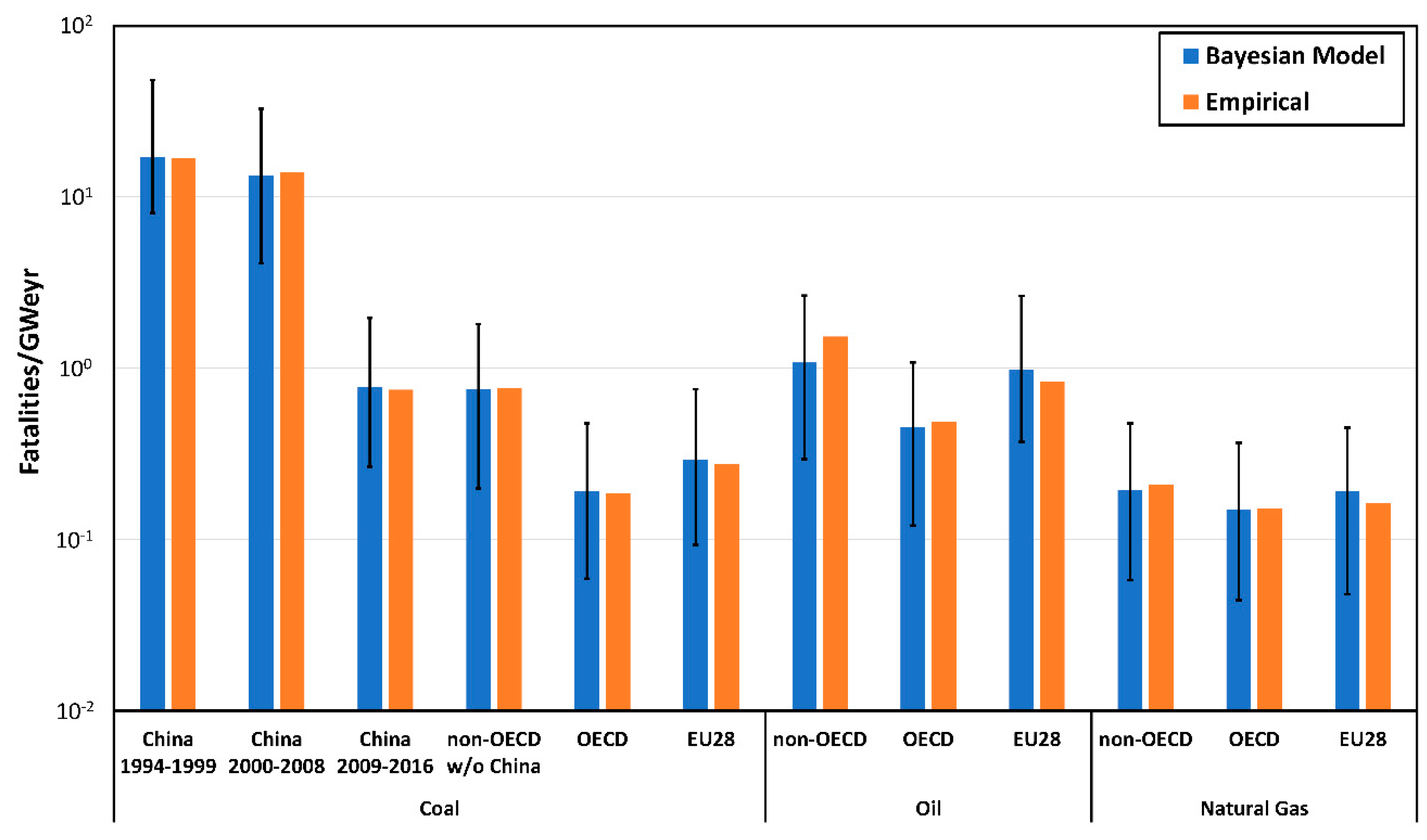
4.3. Risk Assessment for Expected and “Extreme” Scenarios

Finally, the results for accident frequencies (i.e., number of accidents per average annual production in GWeyr) and severity of the resulting consequences (i.e., expected fatalities per accident) were combined to compare overall risk between different energy chains and country groups. Two scenarios were considered, namely, the mean or expected scenario expressed as the expected number of fatalities per GWeyr, and the extreme scenario, defined by the threshold exceeded for a specific return frequency (i.e., exceeded at 1% of the accidents per GWeyr). In both cases, this is done by multiplying the results for frequency in Section 4.1 with the ones for severity in Section 4.2. Both indicators are based on accidents recorded in the period 1970–2016, except for Coal China, where three separate periods (1994–1999, 2000–2008 and 2009–2016) are considered due to different completeness of the datasets. In this context, comparative analysis among expected values could be made taking into account that for all energy chains, unless Coal China, effects such as technological improvements and change in safety regulamentations are not taken into account, while in the Coal China periods, they are potentially affecting the results [20]. Furthermore, to validate the BMA results, the expected fatalities and the fatalities exceeding 1% of the accidents are additionally estimated using an empirical approach. In particular, the validation consists in a check if the results from the empirical approach fall into the confidence levels modelled using the BMA approach. If this is the case, then the BMA result can be considered statistically correct. In terms of empirical analysis, the expected fatalities are estimated as an arithmetical mean, while the fatalities exceeding the 1% of the accidents are estimated as the number of fatalities at the 99% quantile of the historical distribution (Figures S4–S6).

In Figure 3, the expected fatalities per GWeyr are shown. Overall, the results given by the proposed approach are in line with the empirical estimation, since the latter are all located within the credibility interval, proving the validity of the model. Furthermore, this proves the usefulness of the Bayesian analysis, since it can produce results for the entire quantile range, whereas this is not the case for the empirical result. It is interesting to see that in most of the cases the empirical results are very close to the modelled mean risk.

In general, the highest average risk is found for Coal China 1994–1999 followed by Coal China 2000–2008 and Coal China 2009–2016, which is similar to Coal non-OECD w/o China. This indicates that the policy of the Chinese government to close small private mines at the expense of large, state-owned mines leads to improves safety levels [62,63]. For the other energy chains, Oil non-OECD has the highest risk, followed by Oil EU28, Coal China 2009–2016 and Coal non-OECD w/o China. Furthermore, Oil OECD is performing slightly worse than Coal EU28. Natural Gas OECD performs best, followed by Coal OECD, Natural Gas non-OECD and Natural Gas EU28, which perform similarly. These results clearly show that non-OECD countries perform worse than OECD and EU28 as expected. This is caused by a general lack in safety culture with respect to OECD and EU28 countries, which are quite similar. However, it is important to note that although for OECD and EU28 the results are based on sets of data that could be considered complete, non-OECD results are subjected to a potential underreporting. For example, this is expected in the case of Coal non-OECD w/o China, since large coal producers such as India [66] only in recent years initiated a comprehensive and complete recording of accidental events in coal mines [67]. In addition, OECD performs better than EU28 in all the considered energy chains. This is explained by the fact that EU28 is producing significantly less Coal, Oil and Natural Gas than OECD and non-OECD countries (Table 2). Therefore, the expected number of fatalities per production (GWeyr) for the considered energy chains in EU28 are higher than in OECD. Furthermore, among energy chains, Natural Gas is performing generally better compared to Oil and Coal.

Finally, by considering the modelled 5–95% credibility interval, the results show no significant difference in the risk of Coal China 2009–2016 and Coal non-OECD w/o China, Coal OECD and EU28 and Natural Gas for all country groups. This means that by considering either the upper (95%) or the lower (5%) bound, the ranks amongs the abovementioned energy chain and country group combinations do not change. However, significant differences are found between the considered periods for Coal China and the other energy chains and groups. However, when considering the upper bound (95%) for Oil non-OECD, the result is comparable with Coal China 2000–2008, while when considering its lower bound (5%), the result is comparable with Coal China 2009–2016 and Coal non-OECD w/o China. Furthermore, when considering the lower bound of Coal China 2009–2016 and Coal non-OECD w/o China, the results are moving toward the other energy chains and groups, while when considering its upper bound, the risk is moving toward Oil non-OECD, i.e., worsening of its ranking.

In Figure 4 the fatalities exceeded at 1% of accidents per GWeyr are shown. Generally, the empirical results are within the credibility interval modelled using the BMA approach and, thus, validating it. However, in all cases, but for different extents, the empirical results differ from the modelled mean risk. In some cases the empirical results are slightly lower than the mean estimated with BMA (e.g., Coal China 2000–2008). In this case, the difference is strongly related to the significant large number of historical observations with relatively small consequences in the severe context, see Figures S4–S6. In fact, the relatively small consequences of most accidents compensate the few large consequences events along the distribution tail, resulting in a shift of all the quantiles towards a smaller number of fatalities for the 1% quantile. In other words, the value for fatalities exceeding 1% of accidents is moving toward the mean of the distribution, resulting in a lower value for the BMA. This shows the usefulness of the BMA, which accounts for both uncertainty and outliers that strongly affect the empirical approach [68]. In cases where the empirical approach shows slightly higher averages compared to BMA (e.g., Oil non-OECD), its results are strongly affected by few extreme values, which cause a shift of the distributions towards higher quantiles. In fact, the presence of outliers has a significant effect on the empirical mean value, resulting in a large difference to the BMA expected value, where posterior distributions are more resistant to outliers [31].

Overall, the highest average risk occurs with Coal China 1994–1999, followed by Coal China 2000–2008 and by Oil non-OECD. For the other energy chains and country groups, Oil EU28 performs as worst, closely followed by Coal non-OECD w/o China and then by Coal China 2009–2016 and Oil OECD. Furthermore, Natural Gas EU28 performs best, followed by Natural Gas OECD, Natural Gas non-OECD and Coal OECD. Similar to the expected scenario, for each energy chain, non-OECD is performing as worse with respect to OECD and EU28. However, although for OECD and EU28 the results are based on sets of data that could be considered complete, non-OECD results are subjected to a potential underreporting. Furthermore, Natural Gas is generally performing better than Oil and Coal.

Finally, by considering the 5–95% credibility interval, results show no significant difference among OECD and EU28 results for all considered energy chains. Furthermore, no significant difference is also found between the pairs Coal China 1994–1999 and Coal China 2000–2008, Coal China 2009–2016 and Coal non-OECD w/o China.

5. Conclusions

In this study, the Bayesian Model Averaging (BMA) method was implemented for the comparative risk assessment of accidents in fossil energy chains. For this purpose, the BMA framework is applied to comprehensive, global data available from PSI’s ENSAD database. The BMA approach can be used to identify trends and patterns more robustly than classical statistical approaches; nevertheless, interpretation of the results continues to require delving into the underlying data. Furthermore, BMA has the advantage that it allows estimating accident frequencies and severities including uncertainty, expressed in terms of credibility intervals, and dealing with lack of data and lack of knowledge by averaging the posterior distribution over a pre-defined model space. This is of great importance when dealing with complex systems where a “true” model could not be indentified. In fact, BMA allowing the use of multiple models at once implies the possibility to assess the data closer to the “true” model avoiding potential biases of subjective nature intrinsically included in the common method of using a single model defined by experts [23]. Therefore, BMA allows, on the one hand, a general reduction of the uncertainty in the results, which would be beneficial for informed decision-making strategies, and, on the other hand, the consideration of extreme events. In fact, by using a single model to assess the distribution of historical observations might result in a poor fit in the tails due to the presence of few data [24]. In this context, the method proposed in here allows the use of a set of models, which might increase (depending on the complexity of the dataset) the robustness of the risk indicator also for extreme events.

The “top down” approach presented here can also be useful to complement conventional, detailed “bottom-up” models of risk quantification that are commonly used for individual facilities with specific operational processes and site-specific conditions. Ultimately, the developed approach provides a integrated framework that comprehensively covers accident risks in energy chains, and allows estimating specific risk indicators for every quantile of a distribution, including the most extreme (e.g., 95%) where the rare events are expected, and not just for the average as in the case of the empirical approach. Such information are of great interest for different stakeholders and can play an essential role in different decision-making processes. Among others, risk indicators, including their uncertainties, could be used in a holistic sustainability assessment for energy systems, where they are commonly considered in the social pillar of sustainability [1,69]; as indicators for resilience assessment [70]; to assess different types of potential scenarios, i.e., expected and extreme, as input for National Risk Assessment studies [71,72]; for insurance and reinsurance industry purposes such as, for example, to better diversify the reinsurance classifications for different refineries [73]; in other industries purposes such as, for example to regionalize the accident risk for safety assessment purposes [74].

In the second step of the analysis, the frequency and severity distributions were used to compute two distinct risk indicators for the various energy chains (coal, oil, natural gas) and country groups combinations (OECD, non-OECD, EU28). The indicator “expected fatalities per GWeyr” provides an estimate of the average, whereas the indicator “fatalities exceeded in 1% of accidents per GWeyr” represents an extreme risk scenario. Overall, the highest risk was found for both indicators of Coal China in two of the considered periods and Oil non-OECD. However, the decrease in indicators values between Coal China 1994–1999, 2000–2008 and 2009–2016 indicates an improvement in the Chinese coal mines. The closure of small, private mines and strengthening of safety regulations in the past decade are frequently identified as contributors to these safety improvements [62,63]. For the remaining chain and country group combinations, non-OECD generally performed worse than OECD and EU28, except for natural gas where the differences in indicator values were not significant due to generally large uncertainties. In summary, the natural gas chain performs better than the coal and oil chains.

In future work, the scope of the proposed modelling framework will be expanded to cover the following aspects: (1) incorporate other energy chains (e.g., hydropower), for a more comprehensive comparison among energy chains; (2) evaluate additional types of consequences (e.g., injuries), which could also be used for the assessment of, for example, external costs of accidents [20] in a total cost assessment of energy chains or to identify higher external costs of accidents that need to be internalized, for example through insurance, by industries; (3) increase the resolution of risk, i.e., by differentiating it for the different activities within the energy chain, and within each activity, for example, by considering the differentiation in risk among open pit and underground coal mines [75]; (4) extend the BMA framework to spatial problems. i.e., by introducing spatial effects in the model, to be used by industries to identify locations with higher accident risks to mitigate it.

References

1. Roth, S.; Hirschberg, S.; Bauer, C.; Burgherr, P.; Dones, R.; Heck, T.; Schenler, W. Sustainability of electricity supply technology portfolio. Ann. Nucl. Energy 2009, 36, 409–416. [Google Scholar] [CrossRef]
2. Rosner, R.; Burgherr, P.; Spada, M.; Lordan, R. Resilient Energy Infrastructures: Energy Security and Sustainability Implications. In Proceedings of the 6th International Disaster and Risk Conference (IDRC), Davos, Switzerland, 28 August–1 September 2016; pp. 532–535. [Google Scholar]
3. Zio, E. The Future of Risk Assessment. Reliab. Eng. Syst. Saf. 2018, 177, 176–190. [Google Scholar] [CrossRef] [Green Version]
4. Cinelli, M.; Spada, M.; Kadziński, M.; Miebs, G.; Burgherr, P. Advancing Hazard Assessment of Energy Accidents in the Natural Gas Sector with Rough Set Theory and Decision Rules. Energies 2019, 12, 4178. [Google Scholar] [CrossRef] [Green Version]
5. Burgherr, P.; Eckle, P.; Hirschberg, S. Comparative assessment of severe accident risks in the coal, oil and natural gas chains. Reliab. Eng. Syst. Saf. 2012, 105, 97–103. [Google Scholar] [CrossRef]
6. Burgherr, P.; Eckle, P.; Hirschberg, S. Severe accidents in the context of energy security and critical infrastructure protection. In Reliability, Risk and Safety—Back to the Future; Ale, B.J.M., Papazoglou, I.A., Zio, E., Eds.; Taylor & Francis Group: London, UK, 2010; pp. 456–464. [Google Scholar]
7. Burgherr, P.; Hirschberg, S.; Spada, M. Comparative Assessment of Accident Risks in the Energy Sector. In Handbook of Risk Management in Energy Production and Trading; Kovacevic, R.M., Pflug, G.C., Vespucci, M.T., Eds.; Springer: New York, NY, USA, 2013; Volume 199, pp. 475–501. [Google Scholar]
8. Spada, M.; Paraschiv, F.; Burgherr, P. A comparison of risk measures for accidents in the energy sector and their implications on decision-making strategies. Energy 2018, 154, 277–288. [Google Scholar] [CrossRef] [Green Version]
9. Burgherr, P.; Spada, M.; Kalinina, A.; Vandepaer, L.; Lustenberger, P.; Kim, W. Comparative Risk Assessment of Accidents in the Energy Sector within Different Long-Term Scenarios and Marginal Electricity Supply Mixes. In Proceedings of the 29th European Safety and Reliability Conference, Hannover, Germany, 22–26 September 2019; Beer, M., Zio, E., Eds.; Research Publishing: Hannover, Germany, 2019; pp. 1525–1532. [Google Scholar]
10. Edjossan-Sossou, A.M.; Deck, O.; Al Hleib, M.; Verdel, T. A decision-support methodology for assessing the sustainability of natural risk management strategies in urban areas. Nat. Hazards Earth Syst. Sci. 2014, 14, 3207–3230. [Google Scholar] [CrossRef] [Green Version]
11. Novelo-Casanova, D.A.; Suárez, G. Estimation of the Risk Management Index (RMI) using statistical analysis. Nat. Hazards 2015, 77, 1501–1514. [Google Scholar] [CrossRef]
12. Lambrechts, D.; Blomquist, L.B. Political–security risk in the oil and gas industry: The impact of terrorism on risk management and mitigation. J. Risk Res. 2017, 20, 1320–1337. [Google Scholar] [CrossRef] [Green Version]
13. Spada, M.; Ferretti, V. Toward the integration of uncertainty and probabilities in spatial multi-criteria risk analysis: An application to tanker oil spills. In Safety and Reliability—Safe Societies in a Changing World; Haugen, S., Barros, A., Gulijk, C.V., Kongsvik, T., Vinnem, J., Eds.; CRC Press: London, UK, 2018. [Google Scholar]
14. Renn, O. Concepts of Risk: An Interdisciplinary Review. Part 2: Integrative Approaches. GAIA 2008, 17, 196–204. [Google Scholar] [CrossRef]
15. Riddel, M. Uncertainty and measurement error in welfare models for risk changes. J. Environ. Econ. Manag. 2011, 61, 341–354. [Google Scholar] [CrossRef]
16. Cox, L.A., Jr. Confronting Deep Uncertainties in Risk Analysis. Risk Anal. 2012, 32, 1607–1629. [Google Scholar] [CrossRef]
17. Aven, T. On Funtowicz and Ravetz’s “Decision Stake-System Uncertainties” Structure and Recently Developed Risk Perspectives. Risk Anal. 2013, 33, 270–280. [Google Scholar] [CrossRef]
18. Bier, V.M.; Lin, S.-W. On the Treatment of Uncertainty and Variability in Making Decisions About Risk. Risk Anal. 2013, 33, 1899–1907. [Google Scholar] [CrossRef]
19. Pasman, H.; Rogers, W. The bumpy road to better risk control A Tour d’Horizon of new concepts and ideas. J. Loss Prev. Process Ind. 2015, 35, 366–376. [Google Scholar] [CrossRef]
20. Burgherr, P.; Hirschberg, S. Comparative risk assessment of severe accidents in the energy sector. Energy Policy 2014, 74 (Suppl. 1), S45–S56. [Google Scholar] [CrossRef]
21. Härtler, G. Statistische Methoden für die Zuverlässigkeitsanalyse; VEB Verlag Technik: Berlin, Germany, 1983; p. 230. [Google Scholar]
22. Cox, L.A., Jr. Risk Analysis of Complex and Uncertain Systems; Springer: New York, UA, USA, 2009; Volume 129, p. 453. [Google Scholar]
23. Eckle, P.; Burgherr, P. Bayesian Data Analysis of Severe Fatal Accident Risk in the Oil Chain. Risk Anal. 2013, 33, 146–160. [Google Scholar] [CrossRef]
24. Spada, M.; Burgherr, P.; Hirschberg, S. Comparative Assessment of Severe Accidents Risk in the Energy Sector: Uncertainty Estimation Using a Combination of Weighting Tree and Bayesian Hierarchical Models. In Proceedings of the 12th Probabilistic Safety Assessment and Management (PSAM12), Honolulu, HI, USA, 22–27 June 2014. [Google Scholar]
25. Kalinina, A.; Spada, M.; Burgherr, P. Application of a Bayesian hierarchical modeling for risk assessment of accidents at hydropower dams. Saf. Sci. 2018, 110, 164–177. [Google Scholar] [CrossRef]
26. Koch, K.-R. Introduction to Bayesian Statistics; Springer: Berlin, Germany, 2010; p. 250. [Google Scholar]
27. Birrell, P.J.; Ketsetzis, G.; Gay, N.J.; Cooper, B.S.; Presanis, A.M.; Harris, R.J.; Charlett, A.; Zhang, X.S.; White, P.J.; Pebody, R.G.; et al. Bayesian modeling to unmask and predict influenza A/H1N1pdm dynamics in London. Proc. Natl. Acad. Sci. USA 2011, 108, 18238–18243. [Google Scholar] [CrossRef] [Green Version]
28. Apputhurai, P.; Stephenson, A.G. Accounting for uncertainty in extremal dependence modeling using Bayesian model averaging techniques. J. Stat. Plan. Inference 2011, 141, 1800–1807. [Google Scholar] [CrossRef]
29. Leamer, E.E. Specification Searches: Ad Hoc Inference with Nonexperimental Data; John Wiley & Sons Inc.: New York, NY, USA, 1978; p. 370. [Google Scholar]
30. Fragoso, T.M.; Bertoli, W.; Louzada, F. Bayesian Model Averaging: A Systematic Review and Conceptual Classification. Int. Stat. Rev. 2018, 86, 1–28. [Google Scholar] [CrossRef] [Green Version]
31. Shao, K.; Gift, J.S. Model Uncertainty and Bayesian Model Averaged Benchmark Dose Estimation for Continuous Data. Risk Anal. 2013, 34, 101–120. [Google Scholar] [CrossRef]
32. Rios Insua, D.; Banks, D.; Rios, J. Modeling Opponents in Adversarial Risk Analysis. Risk Anal. 2015, 36, 742–755. [Google Scholar] [CrossRef]
33. Dormann, C.F.; Calabrese, J.M.; Guillera-Arroita, G.; Matechou, E.; Bahn, V.; Bartoń, K.; Beale, C.M.; Ciuti, S.; Elith, J.; Gerstner, K.; et al. Model averaging in ecology: A review of Bayesian, information-theoretic, and tactical approaches for predictive inference. Ecol. Monogr. 2018. [Google Scholar] [CrossRef] [Green Version]
34. Raftery, A.E. Bayesian model selection in social research. Sociol. Methodol. 1995, 25, 111–163. [Google Scholar] [CrossRef]
35. Bottolo, L.; Consonni, G.; Dellaportas, P.; Lijoi, A. Bayesian Analysis of Extreme Values by Mixture Modeling. Extremes 2003, 6, 25–47. [Google Scholar] [CrossRef]
36. Bhat, K.S.; Haran, M.; Terando, A.; Keller, K. Climate Projections Using Bayesian Model Averaging and Space–Time Dependence. J. Agric. Biol. Environ. Stat. 2011, 16, 606–628. [Google Scholar] [CrossRef]
37. Zhang, W.; Yang, J. Forecasting natural gas consumption in China by Bayesian Model Averaging. Energy Rep. 2015, 1, 216–220. [Google Scholar] [CrossRef] [Green Version]
38. Zou, Y.; Lord, D.; Zhang, Y.; Peng, Y. Application of the Bayesian Model Averaging in Predicting Motor Vehicle Crashes; Bureau of Transportation Statistics: College Station, TX, USA, 2017.
39. Tsai, F.T.C. Bayesian model averaging assessment on groundwater management under model structure uncertainty. Stoch. Environ. Res. Risk Assess. 2010, 24, 845–861. [Google Scholar] [CrossRef]
40. Jia, W.; McPherson, B.; Pan, F.; Dai, Z.; Xiao, T. Uncertainty quantification of CO2 storage using Bayesian model averaging and polynomial chaos expansion. Int. J. Greenh. Gas Control 2018, 71, 104–115. [Google Scholar] [CrossRef]
41. Dearmon, J.; Smith, T.E. Gaussian Process Regression and Bayesian Model Averaging: An Alternative Approach to Modeling Spatial Phenomena. Geogr. Anal. 2016, 48, 82–111. [Google Scholar] [CrossRef]
42. Reis, D.S., Jr.; Stedinger, J.R. Bayesian MCMC flood frequency analysis with historical information. J. Hydrol. 2005, 313, 97–116. [Google Scholar] [CrossRef]
43. Bailer, A.J.; Noble, R.B.; Wheeler, M.W. Model uncertainty and risk estimation for experimental studies of quantal responses. Risk Anal. 2005, 25, 291–299. [Google Scholar] [CrossRef] [PubMed]
44. Ridout, M.; Demetrio, C.G.B.; Hinde, J. Models for Count Data with Many Zeros. International Biometric Conference; The International Biometric Society: Cape Town, South Africa, 1998; p. 13. [Google Scholar]
45. Parent, E.; Bernier, J. Bayesian POT modeling for historical data. J. Hydrol. 2003, 274, 95–108. [Google Scholar] [CrossRef]
46. Hirschberg, S.; Spiekerman, G.; Dones, R. Severe Accidents in the Energy Sector; Paul Scherrer Institut: Villigen, Switzerland, 1998; p. 340. [Google Scholar]
47. Burgherr, P.; Spada, M.; Kalinina, A.; Hirschberg, S.; Kim, W.; Gasser, P.; Lustenberger, P. The Energy-related Severe Accident Database (ENSAD) for comparative risk assessment of accidents in the energy sector. In Safety and Reliability Theory and Applications; Čepin, M., Bris, R., Eds.; CRC Press: Portoroz, Slovenia, 2017; p. 205. [Google Scholar]
48. Kim, W.; Burgherr, P.; Spada, M.; Lustenberger, P.; Kalinina, A.; Hirschberg, S. Energy-related Severe Accident Database (ENSAD): Cloud-based geospatial platform. Big Earth Data 2018, 2, 368–394. [Google Scholar] [CrossRef] [Green Version]
49. Spada, M.; Burgherr, P.; Boutinard Rouelle, P. Comparative risk assessment with focus on hydrogen and selected fuel cells: Application to Europe. Int. J. Hydrogen Energy 2018, 43, 9470–9481. [Google Scholar] [CrossRef]
50. Burgherr, P.; Hirschberg, S. Assessment of severe accident risks in the Chinese coal chain. Int. J. Risk Assess. Manag. 2007, 7, 1157–1175. [Google Scholar] [CrossRef]
51. Aven, T. The risk concept—Historical and recent development trends. Reliab. Eng. Syst. Saf. 2012, 99, 33–44. [Google Scholar] [CrossRef]
52. British Petroleum Company (BP). BP Statistical Review of World Energy; BP: London, UK, 2018. [Google Scholar]
53. Brooks, S.; Gelman, A.; Jones, G.L.; Meng, X.L. Handbook of Markov Chain Monte Carlo; Chapman & Hall/CRC: Boca Raton, FL, USA, 2011; pp. 1–600. [Google Scholar]
54. Yao, Y.; Vehtari, A.; Simpson, D.; Gelman, A. Using Stacking to Average Bayesian Predictive Distributions (with Discussion). Bayesian Anal. 2018, 13, 917–1007. [Google Scholar] [CrossRef]
55. Wang, C.-P.; Ghosh, M. A Kullback-Leibler Divergence for Bayesian Model Diagnostics. Open J. Stat. 2011, 1, 172–184. [Google Scholar] [CrossRef] [Green Version]
56. Piironen, J.; Vehtari, A. Comparison of Bayesian predictive methods for model selection. Stat. Comput. 2016, 27, 711–735. [Google Scholar] [CrossRef] [Green Version]
57. Watanabe, S. Asymptotic Equivalence of Bayes Cross Validation and Widely Applicable Information Criterion in Singular Learning Theory. J. Mach. Learn. Res. 2010, 11, 3571–3594. [Google Scholar]
58. Wasserman, L. Bayesian Model Selection and Model Averaging. J. Math. Psychol. 2000, 44, 92–107. [Google Scholar] [CrossRef] [Green Version]
59. Andrieu, C.; de Freitas, N.; Doucet, A.; Jordan, M.I. An introduction to MCMC for machine learning. Mach. Learn. 2003, 50, 5–43. [Google Scholar] [CrossRef] [Green Version]
60. Gelman, A.; Rubin, D.B. Inference from Iterative Simulation Using Multiple Sequences. Stat. Sci. 1992, 7, 457–511. [Google Scholar] [CrossRef]
61. Srivastava, R.C. On Some Characterizations of the Geometric Distribution. In Statistical Distributions in Scientific Work; Taillie, C., Patil, G.P., Baldessari, B.A., Eds.; NATO Advanced Study Institutes Series (Series C: Mathematical and Physical Sciences); Springer: Dordrecht, The Netherlands, 1981; pp. 349–355. [Google Scholar]
62. Wu, L.; Jiang, Z.; Cheng, W.; Zuo, X.; Lv, D.; Yao, Y. Major accident analysis and prevention of coal mines in China from the year of 1949 to 2009. Min. Sci. Technol. (China) 2011, 21, 693–699. [Google Scholar] [CrossRef]
63. Geng, F.; Saleh, J.H. Challenging the emerging narrative: Critical examination of coalmining safety in China, and recommendations for tackling mining hazards. Saf. Sci. 2015, 75, 36–48. [Google Scholar] [CrossRef]
64. Trigui, I.; Laourine, A.; Affes, S.; Stephenne, A. The Inverse Gaussian Distribution in Wireless Channels: Second-Order Statistics and Channel Capacity. IEEE Trans. Commun. 2012, 60, 3167–3173. [Google Scholar] [CrossRef]
65. Chhikara, R.S.; Folks, J.L. The Inverse Gaussian Distribution as a Lifetime Model. Technometrics 1977, 19, 461–468. [Google Scholar] [CrossRef]
66. International Energy Agency (IEA). Energy Statistics of Non-OECD Countries; IEA: Paris, France, 2015; p. 771. [Google Scholar]
67. Maiti, J.; Khanzode, V.V.; Ray, P.K. Severity analysis of Indian coal mine accidents—A retrospective study for 100 years. Saf. Sci. 2009, 47, 1033–1042. [Google Scholar] [CrossRef]
68. Thelwall, M. The precision of the arithmetic mean, geometric mean and percentiles for citation data: An experimental simulation modelling approach. J. Informetr. 2016, 10, 110–123. [Google Scholar] [CrossRef] [Green Version]
69. Volkart, K.; Weidmann, N.; Bauer, C.; Hirschberg, S. Multi-criteria decision analysis of energy system transformation pathways: A case study for Switzerland. Energy Policy 2017, 106, 155–168. [Google Scholar] [CrossRef]
70. Gasser, P.; Suter, J.; Cinelli, M.; Spada, M.; Burgherr, P.; Hirschberg, S.; Kadziński, M.; Stojadinovic, B. Comprehensive resilience assessment of electricity supply security for 140 countries. Ecol. Ind. 2020, 110, 105731. [Google Scholar] [CrossRef]
71. Spada, M.; Burgherr, P.; Hohl, M. Toward the validation of a National Risk Assessment against historical observations using a Bayesian approach: Application to the Swiss case. J. Risk Res. 2018, 22, 1323–1342. [Google Scholar] [CrossRef]
72. Federal Office for Civil Protection (FOCP). Disasters and Emergencies in Switzerland: Risk Report 2015; Federal Office for Civil Protection (FOCP): Bern, Switzerland, 2015. [Google Scholar]
73. Burgherr, P.; Cinelli, M.; Spada, M.; Blaszczynski, J.; Słowiński, R.; Pannatier, Y. Risk assessment of worldwide refinery accidents using advanced classification methods: Effects of refinery configuration and geographic location on outcome risk levels. In Safety and Reliability—Safe Societies in a Changing World; Haugen, S., Barros, A., Gulijk, C.V., Kongsvik, T., Vinnem, J., Eds.; CRC Press: London, UK, 2018. [Google Scholar]
74. Burgherr, P.; Spada, M.; Kalinina, A.; Page, P. Regionalized risk assessment of accidental oil spills using worldwide data. In Safety and Reliability of Complex Engineered Systems: ESREL 2015; Podofilini, L., Sudret, B., Stojadinovic, B., Zio, E., Kröger, W., Eds.; CRC Press: Zurich, Switzerland, 2015. [Google Scholar]
75. Spada, M.; Burgherr, P. An aftermath analysis of the 2014 coal mine accident in Soma, Turkey: Use of risk performance indicators based on historical experience. Accid. Anal. Prev. 2016, 87, 134–140. [Google Scholar] [CrossRef]
Figure 1. For each energy chain and country group combination, normalized accident frequencies are reported for the selected set of distributions as well as the Bayesian Model Averaging (BMA) (Average), including mean, 5% and 95% quantiles, and percent contributions (weights).
Energies 13 00295 g001
Figure 2. For each energy chain and country group combination, expected fatalities per accident are shown for the selected set of distributions as well as the BMA (Average), including mean, 5% and 95% quantiles and percent contributions (weights). (a) Expected fatalities in log scale. (b) Fatalities exceeded in 1% of all accidents in log scale.
Energies 13 00295 g002
Figure 3. Risk for the Expected Scenario in terms of fatalities per GWeyr modelled using a BMA and an empirical approach.
Energies 13 00295 g003
Figure 4. Risk for the Extreme Scenario in terms of fatalities per GWeyr modeled using a BMA and an empirical approach.
Energies 13 00295 g004