Article

Energy Modeling of a Refiner in Thermo-Mechanical Pulping Process Using ANFIS Method

1
Department of Mechanical Engineering, School of Engineering, Aalto University, 14400 Espoo, Finland
2
Department of Energy, Lappeenranta University of Technology, 95992 Lappeenranta, Finland
*
Author to whom correspondence should be addressed.
Energies 2020, 13(19), 5113; https://doi.org/10.3390/en13195113
Submission received: 27 August 2020 / Revised: 24 September 2020 / Accepted: 28 September 2020 / Published: 1 October 2020
(This article belongs to the Special Issue Applications of Fuzzy Logic in Renewable Energy Systems)

Abstract

:
In the pulping industry, thermo-mechanical pulping (TMP) as a subdivision of the refiner-based mechanical pulping is one of the most energy-intensive processes where the core of the process is attributed to the refining process. In this study, to simulate the refining unit of the TMP process under different operational states, the idea of machine learning algorithms is employed. Complicated processes and prediction problems could be simulated and solved by utilizing artificial intelligence methods inspired by the pattern of brain learning. In this research, six evolutionary optimization algorithms are employed to be joined with the adaptive neuro-fuzzy inference system (ANFIS) to increase the refining simulation accuracy. The applied optimization algorithms are particle swarm optimization algorithm (PSO), differential evolution (DE), biogeography-based optimization algorithm (BBO), genetic algorithm (GA), ant colony (ACO), and teaching learning-based optimization algorithm (TLBO). The simulation predictor variables are site ambient temperature, refining dilution water, refining plate gap, and chip transfer screw speed, while the model outputs are refining motor load and generated steam. Findings confirm the superiority of the PSO algorithm concerning model performance comparing to the other evolutionary algorithms for optimizing ANFIS method parameters, which are utilized for simulating a refiner unit in the TMP process.

Graphical Abstract

1. Introduction

Due to rising energy prices, environmental concerns, and carbon taxes, energy is becoming one of the critical considerations for large energy consumers [1]. The pulp and paper industry is in the fourth place of the most extensive industrial energy consumer worldwide. The pulp and paper industry contributes to approximately 6% and 2% percent of final industrial energy consumption and carbon dioxide emissions, respectively. In total, 6.87 EJ of total energy consumption was attributed to the pulp and paper industry in 2007 [2,3,4]. Nowadays, thermo-mechanical pulping (TMP) is the most predominant type of mechanical pulping process [5]. Thermo-mechanical pulping is of the extreme energy-intensive processes with a low energy efficiency close to 10 to 15% [6]. Mechanical pulping is an electricity-intensive process in which refiners are the essential units in the pulping process, consuming electricity by the electric motors [2,7,8]. An increase in the electricity price and carbon emission taxes, along with environmental concerns, have committed the pulp mills to increase the energy efficiency to keep their market share and profitability [9,10,11]. In addition, a higher quality of pulp is wanted for pulp mills to retain their position in the competitive market [12]. The refining is declared as the most energy-consuming processes where 80% of the mill total energy consumption is attributed to this process [13]. The refiner is the core and backbone of the thermo-mechanical pulping process. In these hydraulic machines, the rotor and stator crush and beat the pulp fibers in a repeated cycle. Refiners have the same principle for operation; however, they are different in terms of configurations. Wood chips are inserted between two rotating metal discs, and rotary energy is transferred to the pulp by patterned fragments of the plates [14]. Since the refining process is highly affected by different refining variables which are not controllable in some cases such as disturbance variables, it is not an easy task to develop an optimal refining control strategy [15]. In general, the pulp and paper process is highly complicated and integrated. The process consists of several interconnected operations and recycles loops. Moreover, there are many constraints such as fuel and power prices, environmental issues, availability, the performance of equipment, production schedules, and process variability that extremely harden the process of energy optimization in these units [16]. There are several factors such as rotational speed, crossing angle, refining gap, bar dimensions, pulp consistency, etc. influencing the pulp and paper properties. Implementing all these factors into theoretical or thermodynamic equations for defining the refining process (system identification) is approximately impossible. Artificial intelligence (AI) is an alternative powerful data-based method for energy modeling of complicated system and processes. An accurate simulation and prediction of the refining process is achievable by utilizing AI methods.
The majority of the previous studies in the pulp industry have been conducted on the use of analytical methods for the TMP process analysis. Analytical methods like thermodynamic analysis and numerical methods are complicated, time-consuming, and sometimes with low accuracy and hard to employ in many practical applications for complex systems or processes. However, for the initial design of a system where no data is accessible, numerical analysis and experimental models are of high power and value. Khokhar [17] utilized numerical analysis (CFD simulation) to model a simple groove refiner. For the simulation, Khokhar considered pulp as a single-phase Newtonian fluid having 100 times more viscosity comparing to water. Ping et al. [18] used ANSYS CFX to simulate a high consistency refiner for the purpose of reducing refining energy consumption. The findings show an impressive ability of numerical analysis to investigate the torque and pressure of the refiner discs and also calculating refining motor load. Huhtanen and Karvinen [19] studied the performance of non-Newtonian fluid dynamics in papermaking. The purpose of their research is to investigate the application of the non-Newtonian fluid models for simulating the pulp suspension in a turbulent and laminar flow. By studying inter-fiber refining and the energy consumption distribution in the refiner plate gap, Illikainen [14] obtained new information about mechanisms of thermo-mechanical pulp refining in the inner area of a refiner disc utilizing experimental test. Elahimehr et al. [20] introduced an experimental structure to analyze the effect of manipulated refining variables such as the refiner plate gap, dilution water, plate pattern, and speed on the LC refiner performance. Mithrush [21] experimentally investigated the transport phenomena inside a low consistency disc refiner. The main purpose of his research is to examine the effects of operating parameters of refiner on the flow field. Results show a linear relationship between stator backflow velocities and the pressure differential across the refiner.
On the other hand, with the development of artificial intelligence, analyzing complex systems with high accuracy is facilitated [22]. Machine learning is a subdivision of artificial intelligence that is currently undergoing growth and is a very active field in computer science [23]. The purpose of machine learning is to build computer systems learning from experiences and are able to adapt to their surroundings just by relying on data patterns instead [24,25]. In many cases, theoretical modeling of a mechanical system is time-consuming and needs a vast knowledge about the detailed processes happening in the system. On the other hand, the validation of theoretical analyzes is always controversial, and in many cases, requires costly experimental tests. Simula and Alhoniemi [26] performed data-driven analysis for the behavior of a continuous pulp digester. They used a neural network algorithm named Self-Organizing Map (SOM) for the analysis and visualization of high-dimensional data. They revealed the parameter dependencies by implementing the visualizations. Ciesielski and Olejnik [27] applied the neural network approach to predict the paper properties of refined chemical pulp. Their findings confirm a good correlation between the experimental and simulated data. Huaijing [28] used identification technique and time series analysis rather than mechanistic analysis for characterizing system disturbances and to find a dynamic stochastic model to control the two-stage TMP plant. They considered Motor load, Production rate, and refining consistency as manipulated variables to control refining specific energy consumption and refining intensity. Lama et al. [29] performed controllability and resiliency analysis to develop a model of a refining unit to analyze internal interactions that happen in the regulatory operation of TMP refiners. Musavi and Qiao [30] suggested a radial basis function (RBF) neural network for prediction of pulp quality. Their results show significant accuracy in predicting the pulp quality factor ( k # ) in the digester. Molga and Cherbanski [31] conducted research on investigating the ability of the multi-layer networks to simultaneously model the chemical reaction and mass transfer in the liquid-liquid reacting system. They defined the hybrid first principle neural-network model to describe batch and semi-batch stirred tank reactors that operate in different operating conditions. Their proposed approach results in good accuracy and flexibility. Dufour et al. [32] trained a feedforward neural network with a two-layer perceptron for pulp digester to appraise the impact of changes in feedstocks properties.
Understanding and controlling the TMP process is paramount in any pulp and paper industry. In the context of the TMP process, to control the specific energy consumption and pulp quality, it is essential to recognize the non-linear hidden relationships among the refining input and output variables. Therefore it is necessary to have an accurate identification model to adopt an efficient control strategy to handle the process in an optimal way. Accordingly, the main purpose of this research is to develop an accurate refining simulation (identification) model that can be further used for the purpose of energy efficiency analysis and development by implementing an energy-efficient control strategy.
In many cases, industrial processes are complex and are affected by a large number of variables that create a multivariate structure in the problem. However, many producers still practice the traditional univariate statistical process control methods and face difficulties in recognizing the hidden non-linear pattern between process variables. This is while AI methods are proved to have a huge capability to simulate and model multivariate industrial processes such as the thermo-mechanical pulping process. In this study, for the first time, AI methods are proposed and developed to simulate the refining motor load and generated steam of the refiner in the TMP process. To achieve this target, the adaptive neuro-fuzzy inference system (ANFIS) is incorporated with various evolutionary optimization algorithms to obtain the maximum prediction accuracy. The employed evolutionary optimization algorithms are: biogeography-based optimization algorithm (BBO), teaching learning-based optimization algorithm (TLBO), particle swarm optimization algorithm (PSO), genetic algorithm (GA), ant colony (ACO), and differential evolution (DE). Notwithstanding the many studies concerning AI methods, no study has yet been developed to compare the performance of the aforementioned evolutionary algorithms incorporating with ANFIS method.

2. Thermo-Mechanical Pulping Process

Figure 1 shows the schematic of the studied system where a single disc refiner is connected to the heat recovery unit to supply the district heating network from the energy coming from the generated steam during the refining process. The basic target of pulping is to make fibers free from the lignin and then to suspend the fibers in water. Lignin is a natural polymer that fastens the fibers together in wood. In mechanical pulping fibers are separated mainly through mechanical forces. Unlike chemical pulping, mechanical pulping is based more on mechanical forces to develop and separate wood fibers. Refiners are mechanical devices correcting the morphology of fibers in wood. In the refining process, the energy source to apply mechanical force to the pulp is electricity. The large part of electrical energy consumption in refiners electric motor generates heat by producing steam.
The refining dilution water is vaporized by the heat generated in the refiner during the refining process and makes the suspension of chips and water to the fiber–steam suspension [33]. The process becomes more complicated by changes in refining variables such as refiners plate condition (plate erosion) and seasonal variations in raw wood chips composition (such as moist content). Refiner plates are designed to gently soften the lignin in wood pieces and separate the fibers. The typical speed for a refiner rotating plate is about 1200   rpm to 1800   rpm . Refiners plate are controlled precisely to be at the distance of 0.05 2   mm depending on the desired pulp quality and system operating condition [34].

3. Intelligent Method

Machine learning and intelligent techniques are potent approaches to model complex systems as a black box. Among different intelligent learning models, the ANFIS method has a high potential of generating solutions for learning problems with superb accuracy. ANFIS model parameters can be optimized, utilizing optimization algorithms to enhance the efficiency of the prediction. In this study, six different heuristic optimization algorithms have been examined to promote the efficiency of the Anfis method in terms of accuracy in prediction.

3.1. Adaptive Neuro-Fuzzy Inference System (ANFIS)

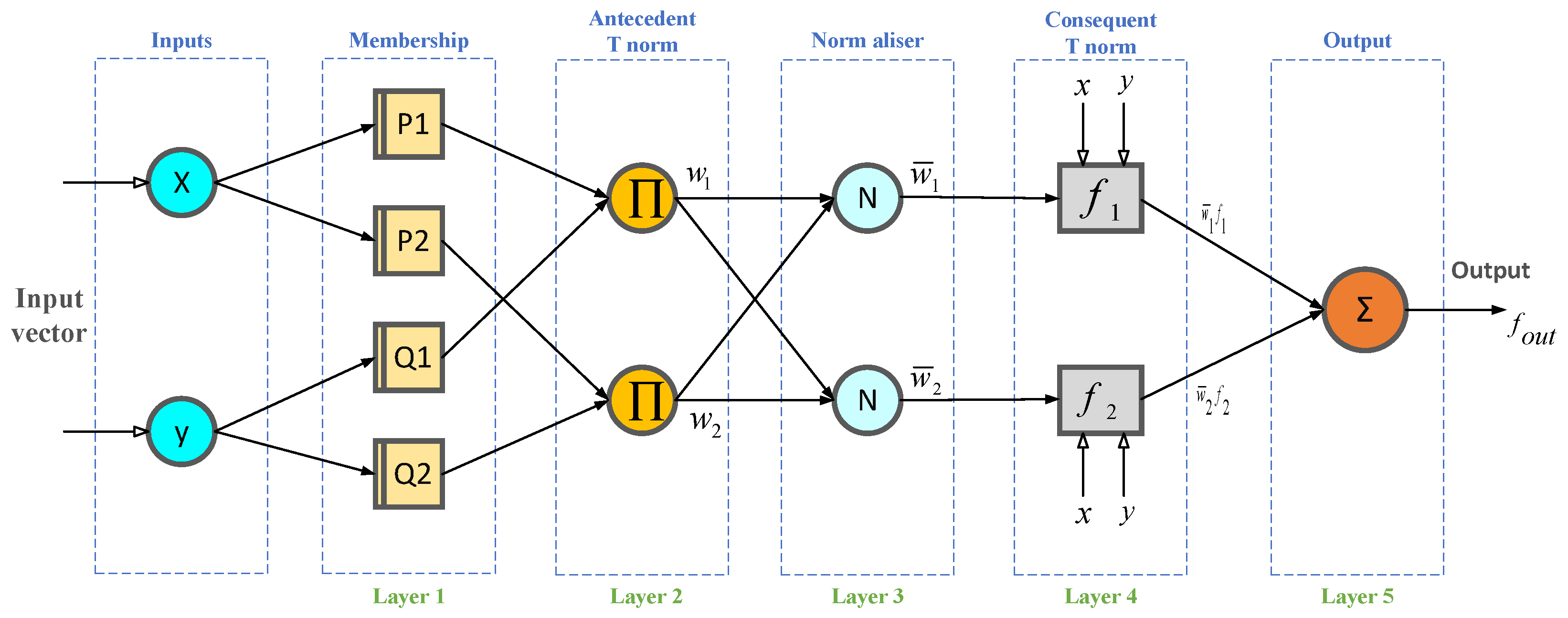
ANFIS method consists of neural networks and fuzzy systems, and defines patterns between the input and output vector by benefiting from the hybrid learning method to determine the optimal distribution of the membership functions [35]. The ANFIS method is constructed by fuzzification, inference engine, and defuzzification [36]. ANFIS method integrates both neural networks and fuzzy logic principle and inherits the advantages of both in a single framework. This method is addressed as a neuro-fuzzy system. Five layers are considered to create the ANFIS inference system. Each ANFIS layer consists of multifold nodes and has been characterized by the node function. The inputs of each layer are determined by the output of the prior layer.
The Sugeno-Takaki model is commonly used to reduce the computational cost as well as pinpointing differences with other models. Two rules for the first order two-rule Sugeno fuzzy inference system is provided in Equations (1) and (2). The neural network and fuzzy system are combined by Radial basis function and Sugeno-Takaki fuzzy inference. Figure 2 illustrates a simplified version of an ANFIS formation, with only two inputs and one output. The adaptive nodes (which are tunable nodes) and fixed nodes are marked as square and circle in Figure 2, respectively [37].
I f   x   i s   P 1   a n d   y   i s   Q 1   f 1 = r 1 x + t 1 y + c 1
I f   x   i s   P 2   a n d   y   i s   Q 2 f 2 = r 2 x + t 2 y + c 2
where A and B are the fuzzy sets, x and y are the ANFIS inputs, f i ( x . y ) is a first-order polynomial regression.
The description of node function for ANFIS layers (presented in Figure 2) is provided in the following. Equations (3) and (4) provide the calculation term for the node’s output in layer 1, which is the fuzzification layer [35].
L O 1 i = μ A j ( x )   ,   f o r   j = 1 , 2
L O 1 i = μ B j 2 ( y )   ,   f o r   j = 3 , 4
where A and B are the semantic tags, x and y are the input nodes, μ x and μ y are membership functions. The Gaussian membership functions are limited from 0 to 1 and presented in Equation (5) or in a different form in Equation (6).
μ ( x ) = 1 1 + ( x c j a j ) 2 b j  
μ ( x ) = exp { ( x c j a j ) 2 }  
In which x is the model input and { a j , b j , c j } are premise parameters. Based on the values of the premise parameters, the membership function’s shape differs. Nodes in layer 2, which is a rule layer, are fixed and determine the firing strength ( w j ) of a rule. Node output is the multiplication of the node input signal (Equation (7)).
L O 2 i = w j = μ A j ( x )   μ B j ( y )   ,   f o r   j = 1 , 2
Layer 3 nodes are fixed node that computes the firing strength of the jth rule to all rules. Equation (8) provides the output of the jth node in layer 3.
L O 3 j = w ¯ j = w j w 1 + w 2   ,   f o r   j = 1 , 2
The Defuzzification layer is layer 4; Equation (9) shows the function of each node in layer 4, consisting of adaptive nodes.
L O 4 j = w ¯ j f j = w ¯ j ( r j x + t j y + c j )   ,   f o r   j = 1 , 2
In which w ¯ i is the layer 3 output, { p i . q i . r i } are the resultant parameters, and f 1 and f 2 are the fuzzy if-then rules (Equations (1) and (2)).
The final output layer is layer 5, where the node sums the receiving signals from layer 4, which is explained in Equation (10).
L O 5 j = w ¯ j f j = j w j f j j w j   = o v e r a l l   o u t p u t ,   f o r   j = 1 , 2
Linear combination of the resulting parameters gives the final output of the ANFIS, which is explained by Equation (11).
f o u t = w ¯ 1 f 1 + w ¯ 2 f 2 = w 1 w 1 + w 2 f 1 + w 2 w 1 + w 2 f 2 = ( w ¯ 1 x ) p 1 + ( w ¯ 1 y ) q 1 + ( w ¯ 1 ) r 1 + ( w ¯ 2 x ) p 2 + ( w ¯ 2 y ) q 2 + ( w ¯ 2 ) r 2

3.2. Biogeography-Based Optimization Algorithm (BBO)

An evolutionary optimization algorithm named Biogeography-based optimization algorithm is inducted from the geographical distribution of biological organisms and is based on the geographical distribution of biological organisms. This optimization algorithm has common features with other biology-based optimization algorithms like particle swarm and genetic algorithm. Therefore, BBO can be used as an alternative solution for the same problems where PSO and GA are employed. For choosing the best solution, the efficiency of these algorithms can be examined. Mathematical models of the biogeography explain the procedure of migration of one species from one island to another, how new species are generated, and how they extinct. The term “island” refers to any habitat that is geographically isolated from other habitats.
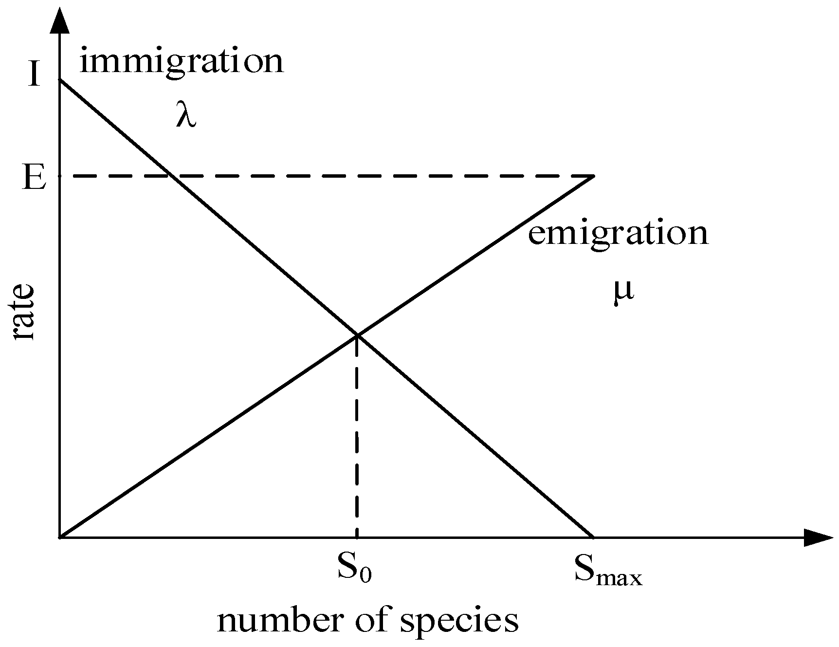
The main parameters of BBO are as follow: habitat suitability index (HIS), the geographical areas that are well-matched for biological species concerning the residence, have a high habitat suitability index (HSI), suitability index variables (SIVs), the immigration rate ( λ ) , the emigration rate ( μ ), the maximum possible immigration rate to the habitat ( I ), the capacity of the habitat to support the species ( S m a x ), the maximum emigration rate ( E ), the balance number of species where immigration and emigration rates are equal ( S 0 ). Figure 3 depicts a model of species abundance in a single habitat. To simplify the species model in a single habitat, immigration and emigration curves are considered to be a straight line, whereas they could be involved curves. Due to the graph, λ   and μ are functions of the number of species in the habitat. The main steps for implementing the BBO algorithm are presented in Figure 4 (further details in [38,39]).

3.3. Teaching Learning-Based Optimization Algorithm (TLBO)

TLBO algorithm was developed by Rao et al. and is a type of evolutionary optimization algorithms. This population-based algorithm is inspired by the effect of a teacher on learners. This method utilizes a population of solutions to obtain a global solution. The individual members of the TLBO algorithm are represented as a group of learners. The algorithm of TLBO is divided into “Teacher Phase” and “Student Phase” part. The process of the TLBO optimization algorithm is outlined in Figure 5. The concept of Teacher Phase originates from the training from the teacher, and the Student Phase is generated by means of learning from the interplay between learners. A desirable teacher is the one who could be able to increase the knowledge of their learners at the same level as themselves. Trainees enhance their knowledge within both the teacher and the learner’s interaction. In [40,41], further details about TLBO can be found.

3.4. Particle Swarm Optimization (PSO)

Particle swarm optimization (PSO) is a heuristic optimization technique which was basically put forward by Kennedy and Eberhart in 1995. The inspiration of the PSO algorithm is relying on the social behavior of birds, insects, and fish and developed from swarm intelligence. To find the foremost solution, several congested particles (candidate solutions) are generated and moved around the search space. The algorithm is launched by producing primitive particles and assessing their preliminary speeds. The movement arrangement of each particle is established on the particle’s experience and the received experience from other particle displacements. The guidance reaches to the swarm when the better sites are identified [42,43]. PSO construction is stated in Figure 6.

3.5. Genetic Algorithm (GA)

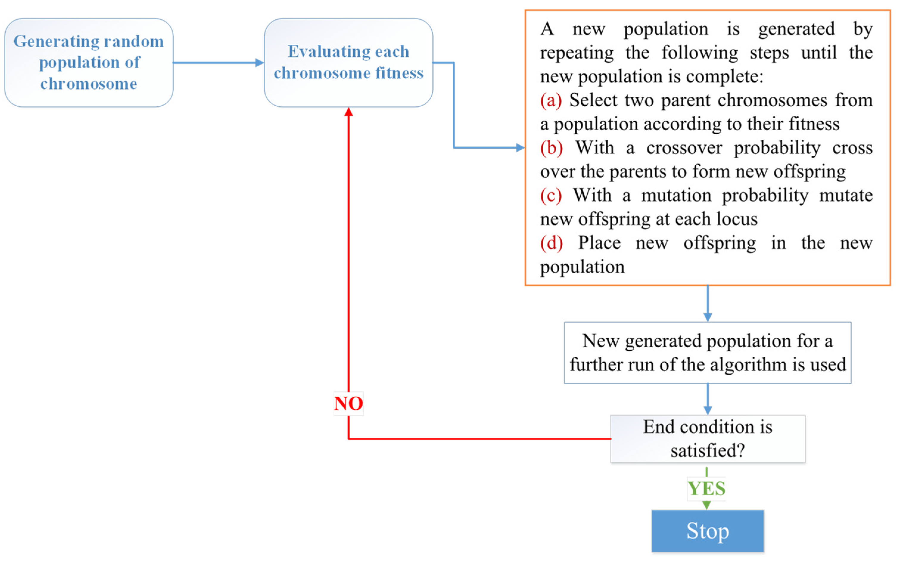
Genetic Algorithm (GA) is a heuristic algorithm commonly used for search and optimization problems, relying on the biological evolution process. In 1960, Holland introduced genetic algorithms based on the evolutionary theory of Darwin. “Natural Selection” and “Genetic Inheritance” are the basic concept for the development of the genetic algorithm. The process begins with a random initial generation of the population and chromosomes as abstract presentations of solution candidates. Population members compete for the right to reproduction. Those who better act in terms of the reduction of the fitness function will be chosen for the next generation. The selection process is organized in a way that only fitter individuals could survive and are selected for the next generation. At the end of each iteration, selected individuals are permitted to generate progeny population for the next iteration of the GA. This iterative behavior is summarized in Figure 7. The optimum solution is obtained after some iterations, where the stopping criteria are satisfied, and the program converges [44,45].

3.6. Ant Colony Optimization Algorithm (ACO)

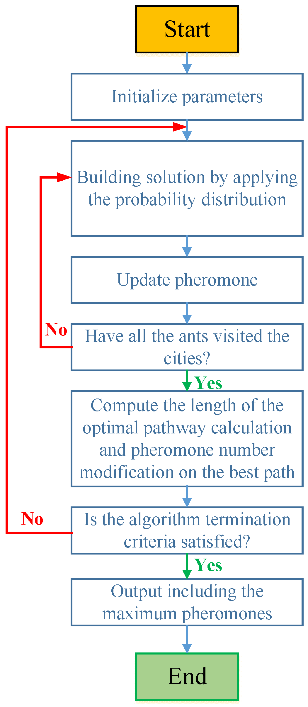
There have been many studies for solving intricate optimization problems by inspiring from complex models of the social habits of animals. Ant colony theory was first introduced by Dorigo in 1992. By the inspiration of the behavior of ant colonies, he proposed an optimization algorithm [46]. The foundation of the ACO algorithm is to detect the most diminutive pathway between the ant den and food. In the food discovering process, some amount of pheromone trail is left by every aunt to facilitate the root identification by others. The probability of a trail to be followed by ants is conditioned on the amount of leaving pheromone. Therefore, the likelihood of choosing pathways with more pheromone is higher. During this process, ants determine the shortest route from the colony to the food sources. The structure of the ACO optimization algorithm is provided in Figure 8.

3.7. Differential Evolution (DE)

Differential evolution (DE) is a sort of metaheuristics method practice to solve the optimization problems (trying to improve the fit solutions), iteratively. This population-based algorithm (presented by Strorn in 1995) has three foremost advantages: independent of the initial parameter values, operating with few control parameters, and fast convergence [47]. DE is a stochastic optimization method and is greatly effective for the optimization problems with non-linear constraints. The main feature that distinguishes DE with other evolutionary algorithms like the genetic algorithm is the mutation arrangement and selection process that form self-adaptive DE [48,49]. Because of the robustness, stability, and ability for global search, DE propelled into one of the powerful optimization algorithms. The iteration of the algorithm starts with four-part: initialization, mutation, crossover, and selection. Different termination criteria like the maximum iterations number, the maximum number of function appraisal, or maximum fulfilling time could be set to stop the process for the optimal solution. Figure 9 provides a flowchart of the DE algorithm [50].

3.8. The Proposed Hybrid Methods for the Refiner Simulation

For the least variation in pulp quality, three input variables could be regulated to control the motor load, pulp consistency, and chip transfer screw speed [51]. The production rate could be simply calculated by multiplying the transfer screw speed ( R ) by a proportionality coefficient. Variation in chip’s density and chip dry solid contents are of the external disturbances affecting the TMP refining process [52].
In this study, to identify the model for predicting motor load and steam generation with the available data sets, four main effective refining variables are taken into account as input parameters of the model. The model input and target variables are provided in Table 1. The AI methods based on the integration of the ANFIS and six different heuristic algorithms are examined to obtain the most accurate system identification. At the first stage of the proposed method, the whole data set is reduced to two-part by creating Train and Test data sets to train the AI network and evaluate the network accuracy, respectively. Training and testing datasets are created to train the data with 70% of the dataset (2952 samples) and test the efficiency of the artificial neural network (ANN) by the remaining 30% of the dataset (1265 samples). From stage 2 to stage 4, the ANFIS model is created, trained, and optimized for the higher accuracy by optimizing the model parameters utilizing six different dominant heuristic optimization algorithms. The final results are evaluated in step 5 to achieve the optimal simulation model. The optimal combination of the ANFIS model and optimization algorithm that has higher accuracy and efficiency is selected as the final model and output of the proposed method. Figure 10 illustrates the proposed data-driven based intelligent simulation approach of the refining process in the thermo-mechanical pulping industry. Descriptions of the performance of each optimization method are provided in previous chapters.
As mentioned in Table 1, The network is constructed based on the ambient temperature ( ) , dilution water ( kg / s ) , plate gap ( mm ) , and chip transfer screw speed (rpm) as input variables (predictive variables), where, except the ambient temperature, other input variables could be considered manipulated variables. The mentioned variables are used to determine refining motor load ( MW ) and refining produced steam (kg/s). A comprehensive dataset with a wide range of variation is provided for this investigation.
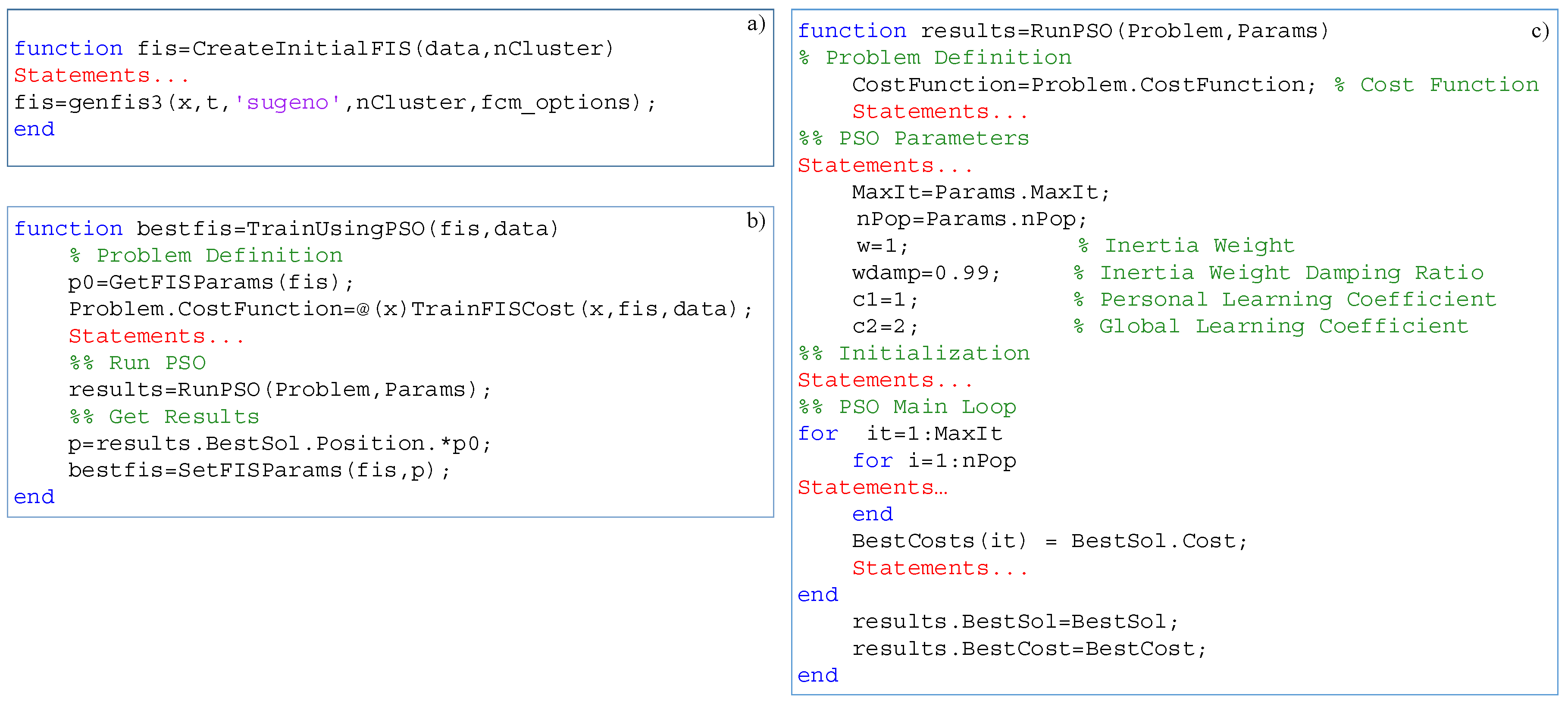
“CreateInitialFIS” function is employed to build an initial fuzzy inference system (FIS) for the model. The fuzzy inference system is constructed based on genfis3 in MATLAB software library (Figure 11a). The concept of fuzzy c-means (FCM) clustering is practiced to model the data behavior where a set of rules are cited. Khosravi et al. [53] compared three types of ANFIS, including ANFIS-FCM (fuzzy c-means), ANFIS-SC (subtracting clustering), and ANFIS-GP (grid partitioning). They reported that ANFIS-FCM performs better than the ANFIS based on SC and GP. For this reason, in this study, the ANFIS model was created based on genfis3 (FCM) in Matlab Software with the number of clusters of 10.
The number of clusters and input data is the input argument of the created function. The AI model is trained by employing different evolutionary algorithms (step 4 in Figure 10). For instance, Figure 11b presents the function of Train Using PSO. The objective of the process is to define the optimum FIS parameters. p 1 0 , p 2 0   ,     ,   p n 0 are the primary values of FIS parameters, while p 1 , p 2   ,     ,   p n introduce the optimal parameters. Equation (12) describes the optimization problem. The finest x value is specified utilizing an evolutionary optimization algorithm (Figure 11c).
p i = x i p i 0

4. Results and Discussion

Empirical models derived from previous studies have been used to validate the measured data. This procedure is described in the data validation section, and in the next section, the artificial intelligence modeling results are presented and discussed.

4.1. Data Validation

In previous researches, plate gap, dilution water, and refining production rate are considered to be key variables to model and simulate the refining energy consumption. The following empirical equation introduces motor load as a function of the refining dilution water flow rate, refining plate gap, and refining production rate [54,55].
M L ( p r , P G , D W ) = k m × Pr D W ( 1 exp ( 10 × P G ) ) ( a b × P G )
In which M ( MW ) is the refining motor load, G ( mm ) is the plate gap, D ( L / min ) is the refining dilution water flow rate, and k m , a and b are parameters of the refiner and belong to the working conditions and the technical characteristics of the refiner.
To validate the measured data, Equation (13) is considered as a reference non-linear regression model [55], which relates the three-input variables to the refining motor power. Since regression coefficients in Equation (13) are specific for each refiner, each of the three regression coefficients is optimized using the genetic optimization algorithm for the least mean absolute percentage error ( M A P E ) .
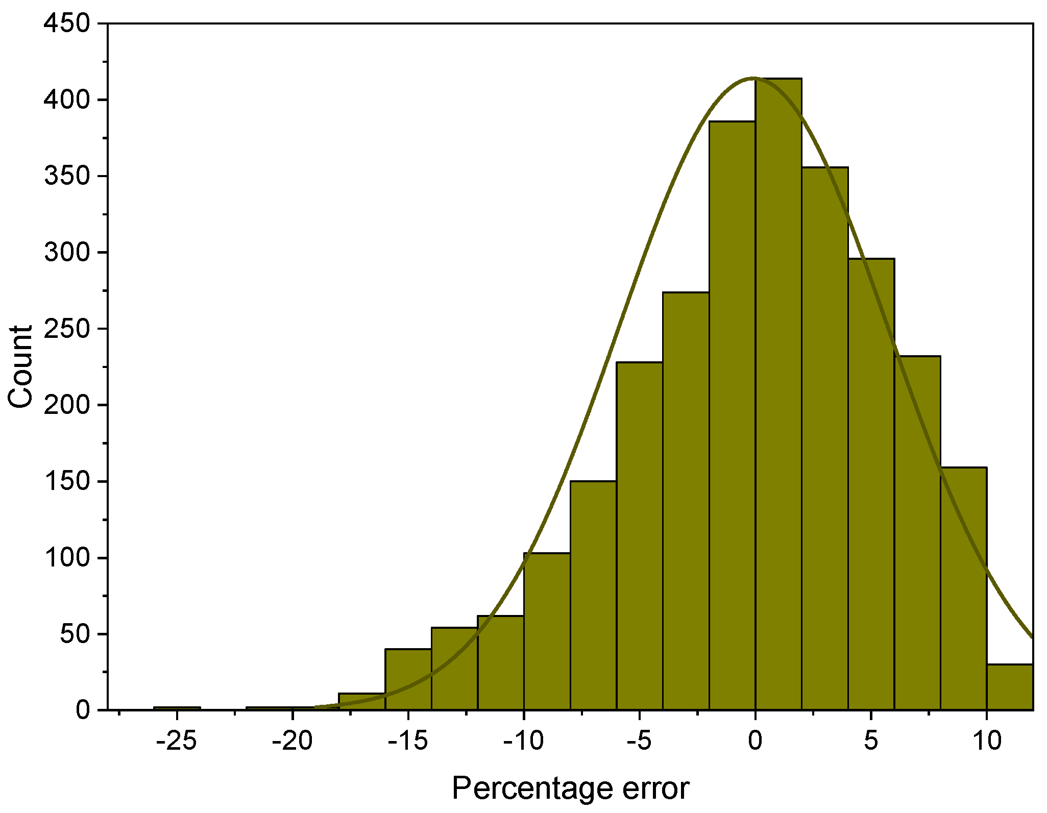
The correlation coefficient ( R ) , mean absolute percentage error ( M A P E ) , and root mean square error ( R M S E ) are used as three criteria for the regression model analysis (Equations (14)–(16)). Table 1 represents the non-linear model specifications for the best fit. Results show that the experimental data are reliable and validated with the empirical model. Table 2 tabulates the evaluation criteria for analyzing the efficiency of the non-linear regression model in predicting refining motor load as well as obtained optimal regression model coefficients from fitting data to the Equation (13). This fact indicates the validity of the measured data for further analysis. In this regard, Figure 12 reports the percentage error histogram of the validated non-linear regression model.
R = i = 1 n ( r i r ¯ ) ( p i p ¯ ) i = 1 n ( r i r ¯ ) i = 1 n ( p i p ¯ )
M A P E = 1 n i = 1 n | r i p i | | r i |
R M S E = 1 n i = 1 n ( r i p i ) 2
where r i ,   p i ,   r ¯ ,   p ¯ , and n are real (target) data, predicted data, an average of target data, average of estimated data, and the quantity of data, respectively.

4.2. Models Comparison

Given that different heuristic optimization algorithms have been investigated to heighten the performance of the ANFIS model, good insight into the efficiency of different optimization methods is essential. For this purpose, the performance indicators of different methods are evaluated in the following. Three performance indicators, namely correlation coefficient ( R ) , mean-squared error ( M S E ) , and root-mean-square error ( R M S E ) are considered as criteria for appraising the precision of the different optimization methods for the best prediction.
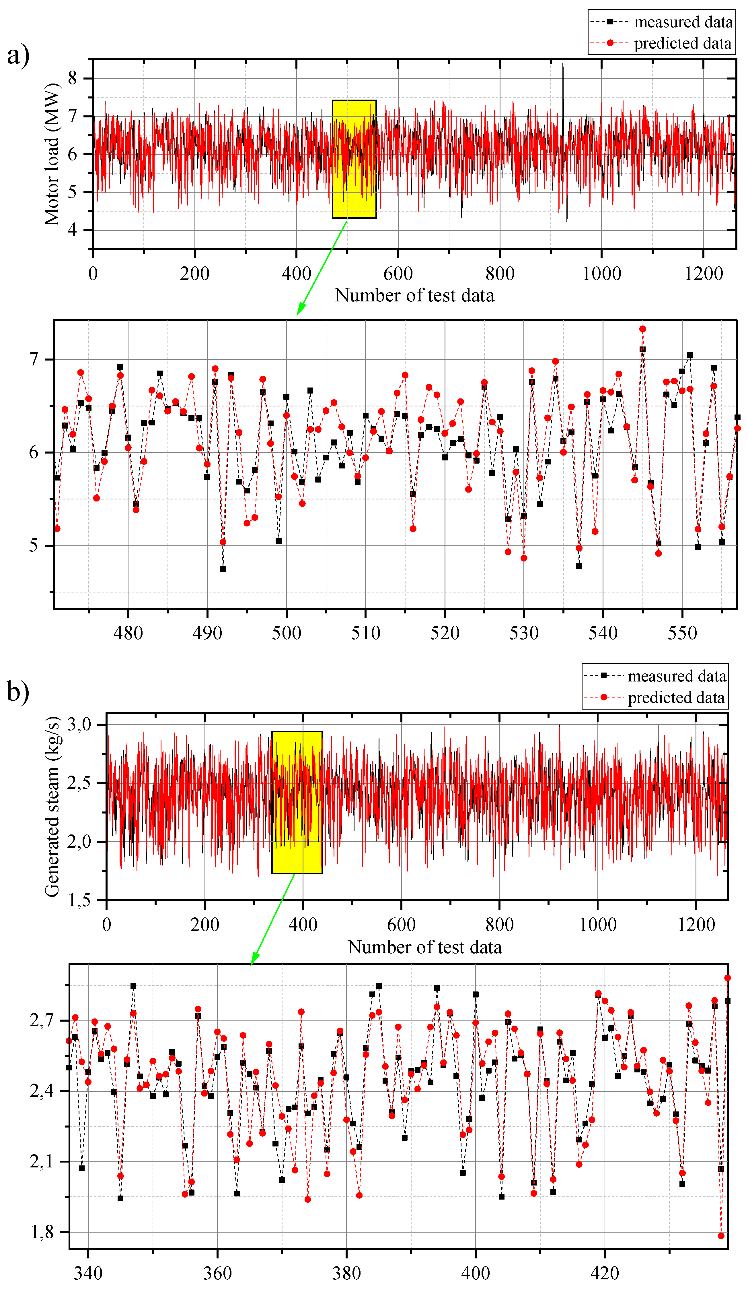
Figure 13 shows the test samples of the BBO algorithm combined with ANFIS to predict the refining motor load electricity consumption (a) and refining generated steam in the refining process (b). Every test data marked as the x-axis in the graph is estimated by a combination of four different variables named ambient temperature, rotor gap, production rate, and dilution water flow rate. The predicted and measured data for motor load and generated steam are given on Y-axis. The lower discrepancy between the measured and estimated data indicates a higher performance and accuracy of the model. The BBO algorithm was implemented based on the following technical parameters: Keep rate =   0.2 ; Number of kept habitats = r o u n d   ( k e e p   r a t e × n u m b e r   o f   t h e   p o p u l a t i o n ) ; Number of new habitats =   n u m b e r   o f   p o p u l a t i o n n u m b e r   o f   k e p t   r a t e . For all models, the number of the population and the number of iterations are considered as 500 . The statistical criteria for the prediction assessment of the BBO model were obtained as: for predicting the motor load, train samples, R M S E   =   0.3235   MW , R   =   0.8590 , and M S E   =   0.1046   MW 2 ; test samples, R M S E   =   0.3235   MW , R   =   0.8590 , and M S E   =   0.1046   MW 2 . To estimate the steam generation, train samples, R M S E   =   0.1319   kg / s , R   =   0.8689 and M S E   =   0.0174   kg 2 / s 2 ; test samples, R M S E   =   0.1325   kg / s , R   =   0.8682 and M S E   =   0.0175   kg 2 / s 2 .
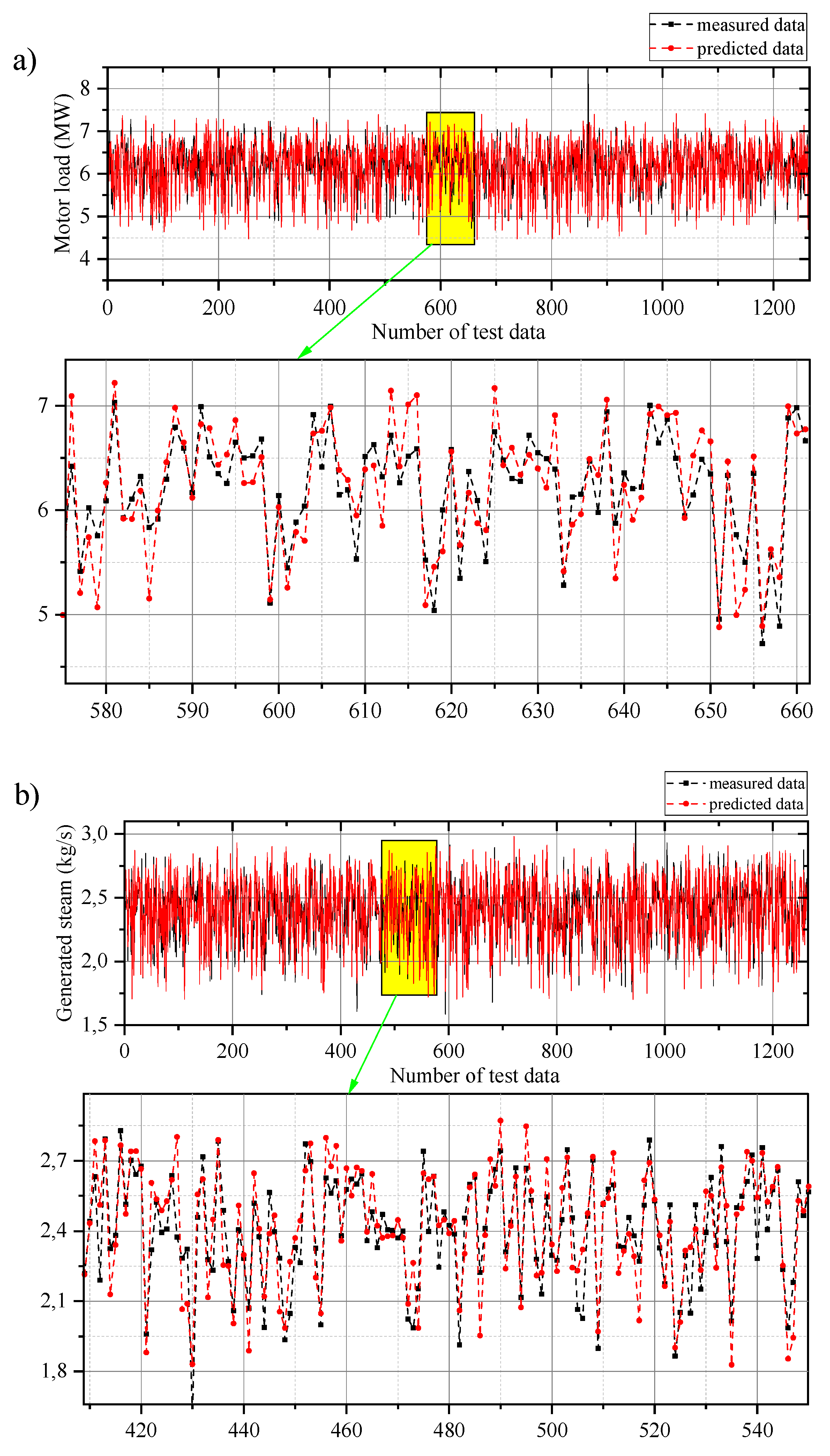
Regarding the accuracy of the model-based-TLBO algorithm, Figure 14 provides a general view of the test data. The TLBO algorithm is a robust and effective optimization method, developed based on the teaching process. In contrast to other evolutionary algorithms, TLBO does not require to adjust any controlling parameters. Two primary stages considered to implement the TLBO algorithm are “teacher phase” and “learner phase.” As stated earlier, three statistical indicators are taken into account to evaluate the accuracy of different models. Prediction performance of the model for estimating the motor load is R M S E   =   0.3488   MW , R   =   0.8472 , and M S E   =   0.1216   MW 2 ; and for predicting the steam generation was R M S E   =   0.1487   kg / s , R   =   0.8607 and M S E   =   0.0211   kg 2 / s 2 for the test data.
Figure 15 delineates the measured data and predicted data for the model PSO-based model testing phase. The model results in a low root mean squared and squared error. The controlling parameters for the PSO algorithm are: inertia weight =   1 , personal learning coefficient =   1 , global learning coefficient = 2 . This model predicted the targets (for the test samples and respectively for motor load and steam generation with R M S E   o f   0.2712   MW and 0.1131   kg / s ; M S E   o f   0.0735   MW 2 and 0.0128   kg 2 / s 2 ; and   R of 0.9052 and 0.9032 .
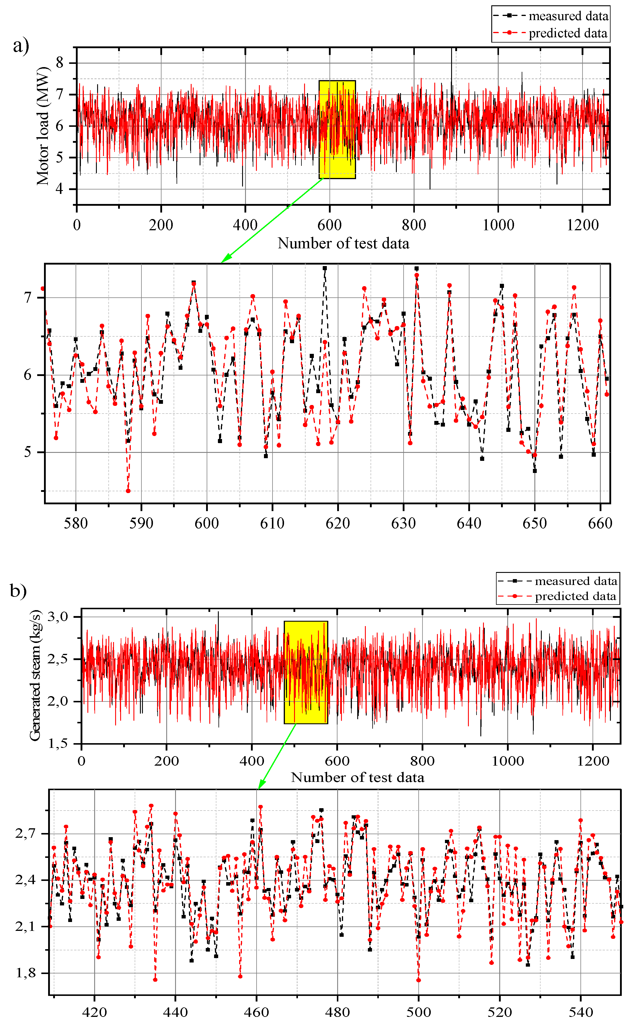
Figure 16 depicts the prediction performance of the GA algorithm for predicting the motor load (a) and produced steam (b) using different input variables. The GA was implemented based on the following structure: crossover percentage =   70 % , mutation percentage =   50 % , mutation rate =   10 % , and selection pressure = 8. The model predicted the motor load with 0.3081 MW RMSE, 0.8677 R and 0.094   MW 2   M S E and estimated the produced steam with 0.1269   kg / s   R M S E , 0.8804   R , and 0.0161   kg 2 / s 2   M S E (for test data).
Based on testing datasets, Figure 17 illustrates the measured and predicted data, employing an ACO-based model. The ACO algorithm was built by an intensification factor of 0.5 and zeta (deviation-distance ratio) of 1. With this structure, predicted data follow the observed data with the R M S E of 0.3416 MW and 0.1362 kg / s ; R of 0.8430 and 0.8624 ; and M S E of 0.1167   MW 2 and 0.01856 kg 2 / s 2 , for motor load and generated steam, respectively.
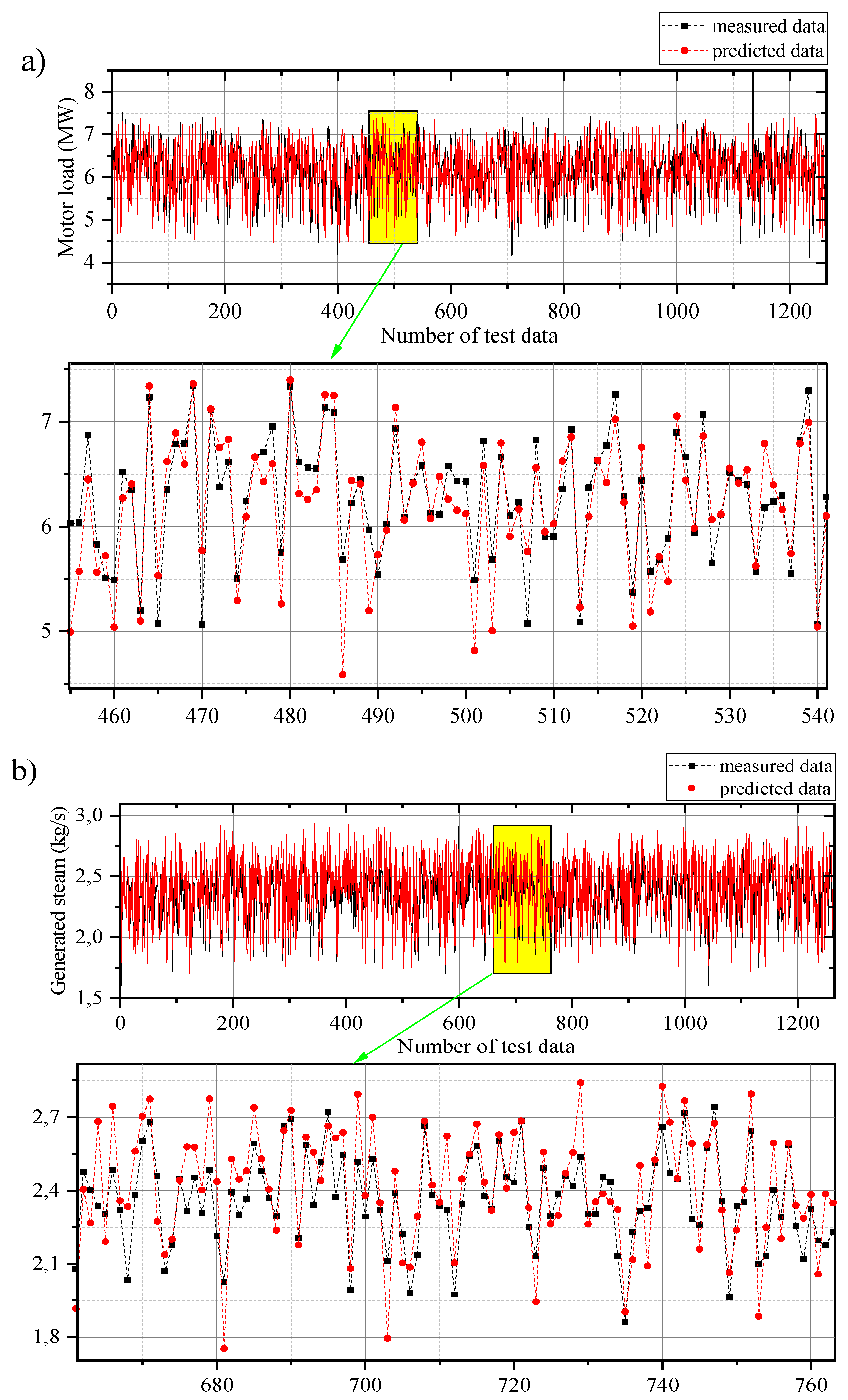
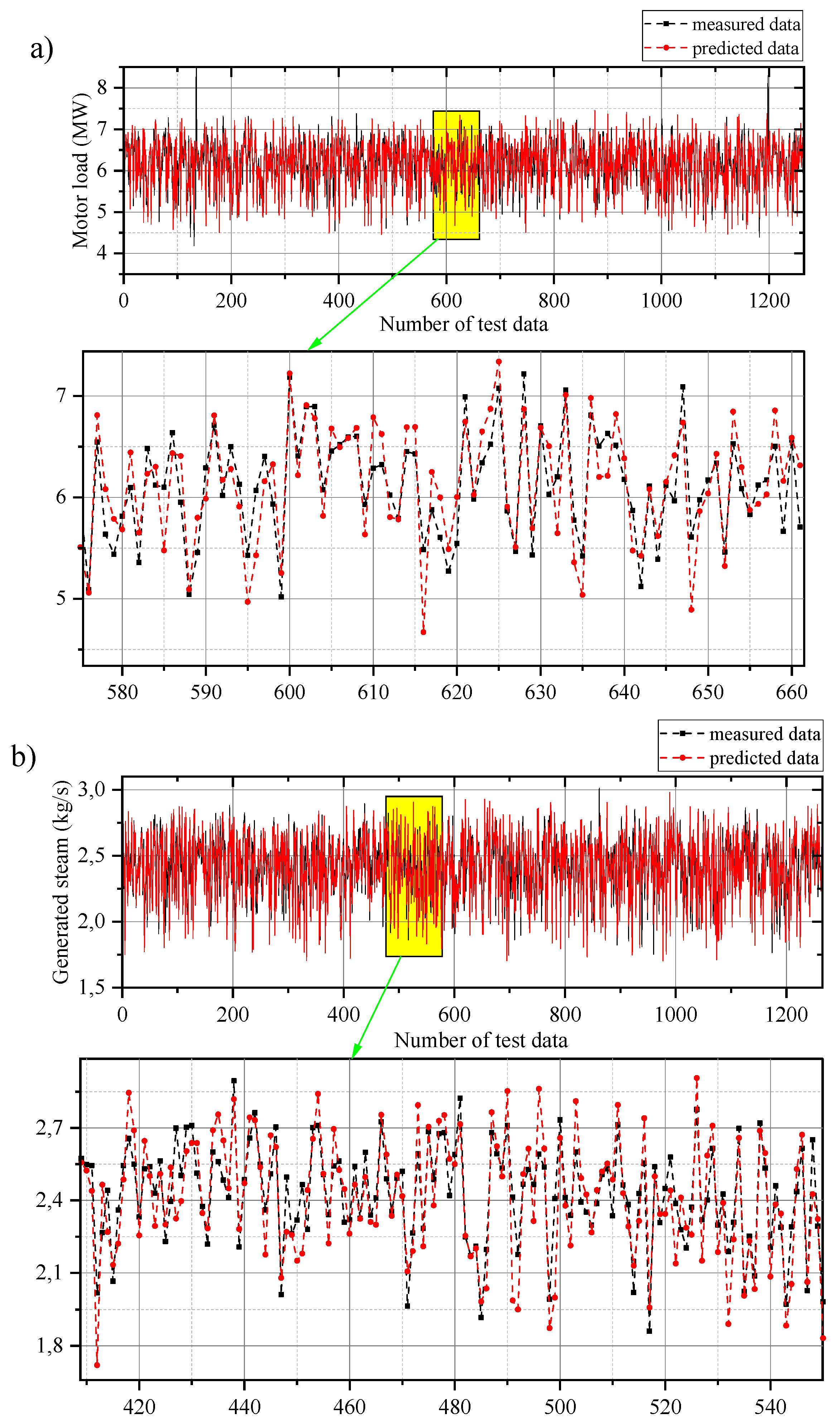
The test phase of the DE method for estimating the targets is shown in Figure 18. The DE parameters have crossover probability =   0.1 , lower bound of scaling factor =   0.2 , and upper bound of scaling factor =   0.8 . With regard to tracking the measured data, the intelligent model follows the measured data accurately, and the statistical parameters were obtained as R M S E   =   0.3398   MW , R   =   0.84 and M S E   =   0.1155   MW 2 (for motor load) and R M S E   =   0.1303   kg / s , R   =   0.8710 and M S E   =   0.0169   kg 2 / s 2 (for generated steam).
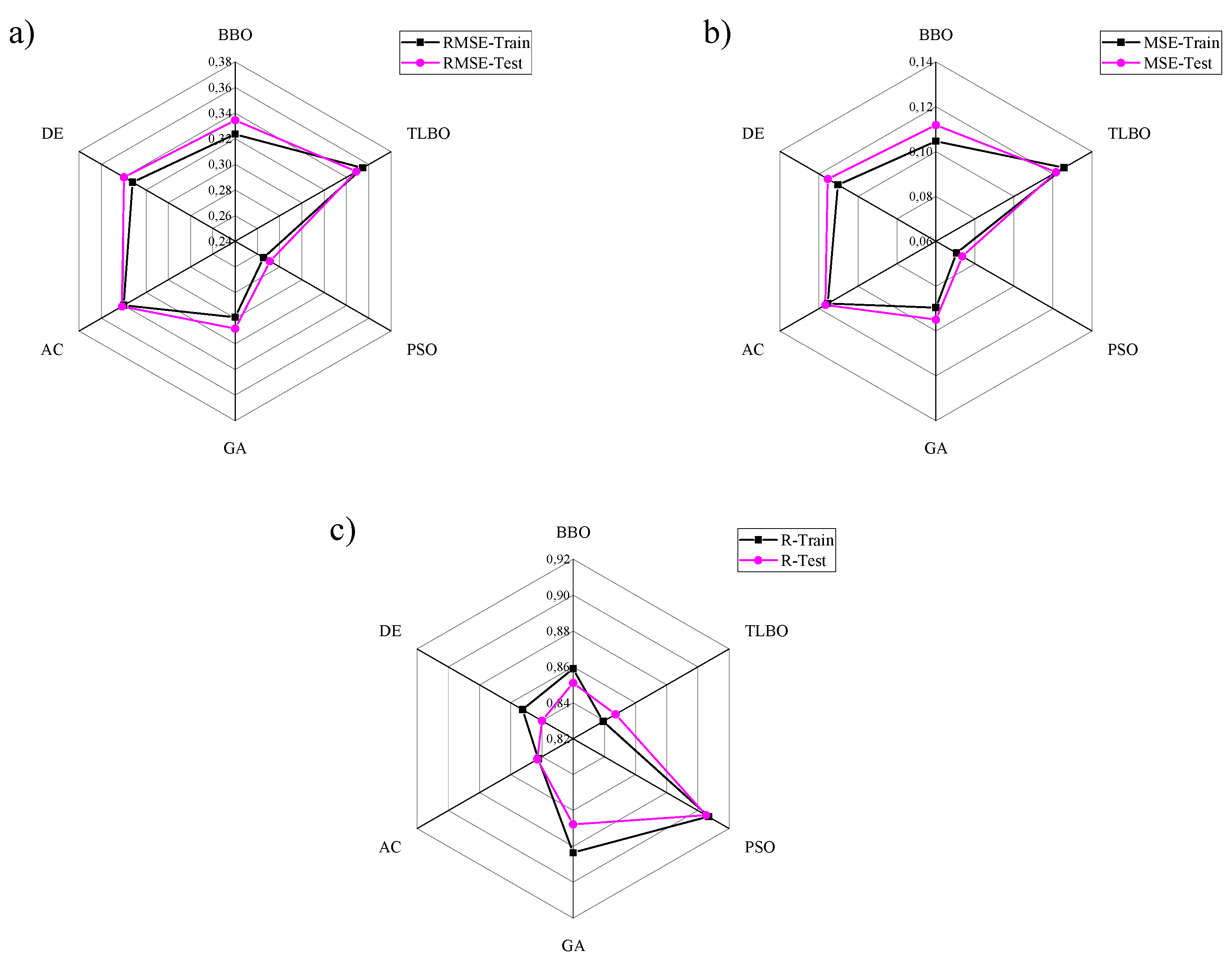
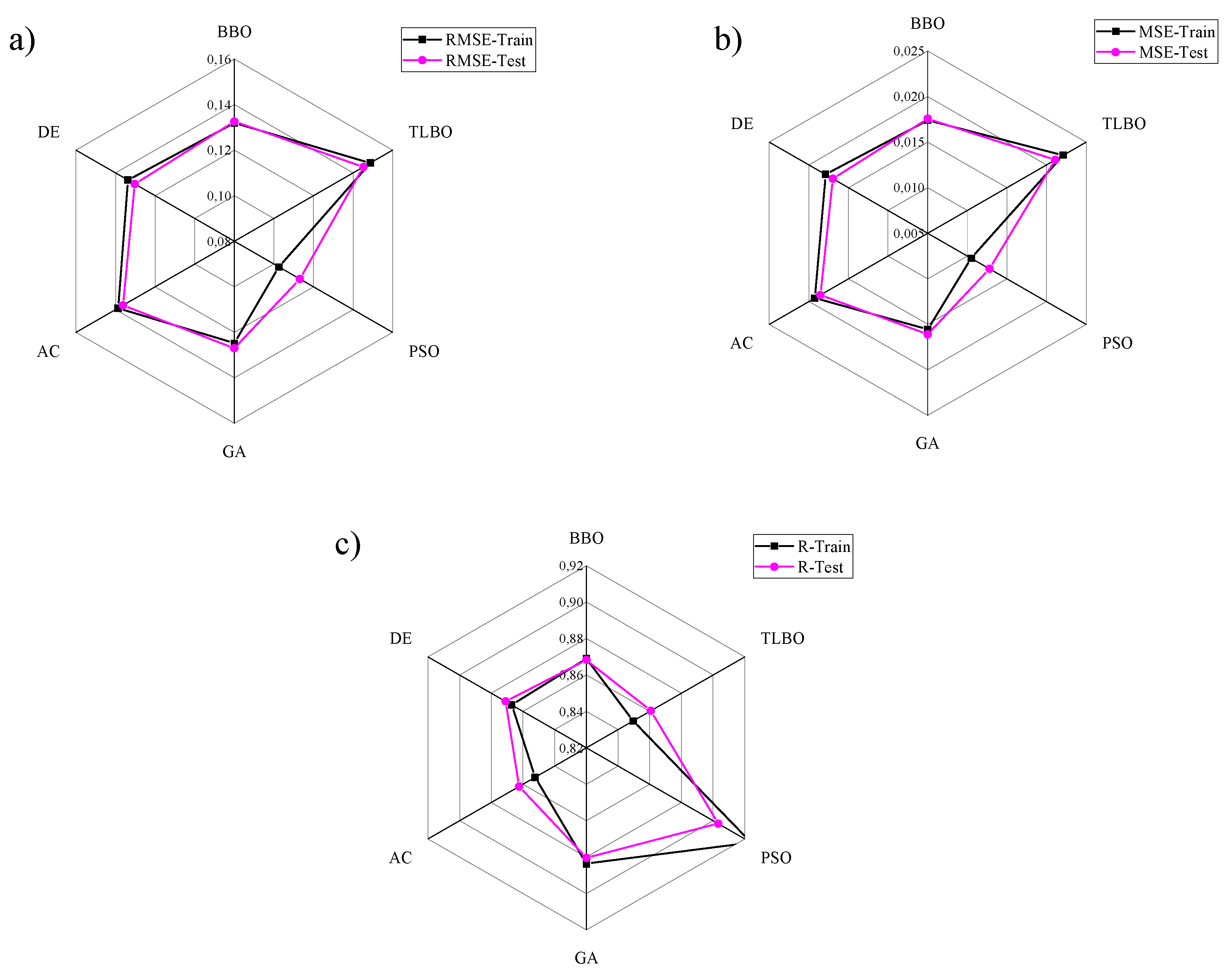
Figure 19 reports the statistic indicators of the six studied models attributing to implement different heuristic optimization algorithms to the ANFIS method for motor load and Figure 20 for generated steam prediction. In order to tabulate the data regarding the refining motor load and generated steam models evaluation criteria in Figure 19 and Figure 20, Table 3 and Table 4 are provided to address the real values of the mentioned variables. For both motor load and generated steam, the PSO algorithm works best in terms of the correlation coefficient ratio, which is 0.9052 for motor load and 0.9032 for generated steam, respectively. The TLBO algorithm shows the weakest performance in R-value. 0.8472 for motor load and 0.8607 for generated steam prediction are the value of the correlation coefficient (R) resulted from the TLBO optimization algorithm integrated to ANFIS. On the other hand, the results for both root mean squared error and mean squared error show similar behavior as the R criterion. So that the PSO algorithm results in the best and the TLBO algorithm in the worst performance for the error criteria. For instance, the RMSE value in motor load prediction is 0.2712   MW for the PSO algorithm and 0.3488   MW for the TLBO algorithm, which respectively shows the best and worst performances in RMSE value. This behavior is also true for the MSE index, as same as RMSE. Such a way that, MSE value for generated steam prediction is 0.0128   kg 2 / s 2 for the PSO algorithm and 0.0211   kg 2 / s 2 for the TLBO algorithm, which is approximately two times greater than the PSO one. Thus, the combination of the ANFIS method and the PSO optimization algorithm determines the best model for predicting motor power consumption and produced steam in the refining process. This model results in better model accuracy evaluation criteria, which imply to be the most suitable model for the purpose of energy efficiency analysis and implementing optimal refining control strategy.

5. Conclusions

TMP process is the most dominant refiner-based mechanical pulping process. Due to harsh conditions inside the pulp refineries, modeling and predicting what exactly is happening during the crushing/beating process is at stake. The efficient mechanism for fiber development is not yet introduced, and mechanical energy transformation to the pulp is not apparent. There are several factors such as rotational speed, crossing angle, refining gap, bar dimensions, and pulp consistency influencing the pulp and paper properties. Implementing all these factors in theoretical or thermodynamic equations for defining the refining process is approximately impossible. Employing an optimal refining control strategy involves system identification, and the more accurate the process simulation model, the more efficient the process control. For this reason, the key objective of this study is to achieve an accurate system identification model for modeling the amount of energy consumed and steam produced in the refining process of thermo-mechanical pulp mill using artificial intelligence methods. Artificial intelligence is an alternative powerful data-based method. Thanks to the now-fast CPUs and high capacities of memories, it is possible to have an accurate prediction of the refining process by employing AI methods. In this research, the refining process is simulated through the hybrid intelligence approach. ANFIS method is used for data training. The efficiency of the six different evolutionary optimization algorithms has been investigated to optimize the network parameters. The PSO and the TLBO algorithm have the best and weakest result in terms of efficiency for optimizing ANFIS parameters both for the objective refining motor load and generated steam prediction, respectively. The model correlation coefficient and root-mean-square error of the optimized model with the PSO algorithm are 0.9052 , 0.2712   MW for motor load prediction, and 0.9032 , 0.1131   kg / s   for generated steam prediction. Another accomplishment of this study is the achievement of a more comprehensive model of the refining process than existing models. For instance, in the available models in the literature, the effect of site ambient temperature on motor load or the effect of refining variables to the steam produced during the refining process has not been investigated. While in this research with the aid of artificial intelligence, a general model for determining the relation of the four different affecting variables (as input variables) to the generated heat and motor load (as output variables) is created. This model can be later used to analyze and improve the energy efficiency of the TMP process by adopting a proper refining control strategy.

Author Contributions

Conceptualization, methodology, writing-original draft, formal analysis, B.T.; formal analysis, software, writing—review & editing, A.K.; data curation, funding acquisition, project administration, supervision, T.L.; conceptualization, investigation, funding acquisition, supervision, H.H.; writing—funding acquisition, E.V.; funding acquisition, supervision, project administration, writing—review & editing, S.S. All authors have read and agreed to the published version of the manuscript.

Funding

The authors gratefully acknowledge the support of the Academy of Finland, grant number 315020.

Conflicts of Interest

The authors declare no conflict of interest.

Nomenclature

TMPThermo-mechanical pulpingVariables
BBOBiogeography-based optimization algorithmMSEMean-square-error
GAGenetic algorithmRMSERoot-mean-square error
PSOParticle swarm optimization algorithmMAPEMean-absolute percentage error
DEDifferential evolution R Correlation coefficient
ACOAnt colony optimization algorithm R 2 Determination coefficient
TLBOTeaching learning-based optimization algorithm M L ( MW ) Refining motor load
ANFISAdaptive neuro-fuzzy inference system D W ( L / min ) Refining dilution water flow rate
RBFRadial basis function P G ( mm ) Refining plate gap
LCLow consistency P r Refining production rate

References

  1. Talebjedi, B.; Behbahaninia, A. Availability analysis of an Energy Hub with CCHP system for economical design in terms of Energy Hub operator. J. Build. Eng. 2021, 33, 101564. [Google Scholar] [CrossRef]
  2. Bajpai, P. Pulp and Paper Industry. In Energy Conserv, 1st ed.; Elsevier: Amsterdam, The Netherlands, 2016. [Google Scholar]
  3. Akhtar, M.; Scott, G.M.; E Swaney, R.; Shipley, D.F. Biomechanical pulping: A mill-scale evaluation. Resour. Conserv. Recycl. 2000, 28, 241–252. [Google Scholar] [CrossRef]
  4. Corcelli, F.; Ripa, M.; Ulgiati, S. Efficiency and sustainability indicators for papermaking from virgin pulp—An emergy-based case study. Resour. Conserv. Recycl. 2018, 131, 313–328. [Google Scholar] [CrossRef]
  5. Gullichsen, J.; Paulapuro, H.; Sundholm, J. Thermomechanical pulping. In Papermaking Science and Technology, Book 5: Mechanical Pulping; Fapet Oy: Jyväskylä, Finland, 1999; pp. 159–218. [Google Scholar]
  6. Ottestam, C.; Salmén, L. Fracture energy of wood; relation to mechanical pulping. Nord. Pulp Pap. Res. J. 2001, 16, 140–142. [Google Scholar] [CrossRef]
  7. Holmberg, J.M.; Gustavsson, L. Biomass use in chemical and mechanical pulping with biomass-based energy supply. Resour. Conserv. Recycl. 2007, 52, 331–350. [Google Scholar] [CrossRef]
  8. Fracaro, G.; Vakkilainen, E.; Hamaguchi, M.; Souza, S.N.M. Energy Efficiency in the Brazilian Pulp and Paper Industry. Energies 2012, 5, 3550–3572. [Google Scholar] [CrossRef]
  9. Johansson, O.; Jackson, M.; Wild, N.W. Three steps to improved TMP operating efficiency. In International Mechanical Pulping Conference; TAPPI: Peachtree Corners, GA, USA, 2007; pp. 356–369. [Google Scholar]
  10. Machani, M.; Nourelfath, M.; D’Amours, S. A mathematically-based framework for evaluating the technical and economic potential of integrating bioenergy production within pulp and paper mills. Biomass Bioenergy 2014, 63, 126–139. [Google Scholar] [CrossRef]
  11. Baruah, D.; Baruah, D.; Hazarika, M.K. Artificial neural network based modeling of biomass gasification in fixed bed downdraft gasifiers. Biomass Bioenergy 2017, 98, 264–271. [Google Scholar] [CrossRef]
  12. Strand, B.C.; Fralic, G. May. Economic benefits from advanced quality control of TMP mills. In Control Systems, Preprints, Conference; Control Systems Conference 2000, 2000; pp. 11–15. [Google Scholar]
  13. Rudie, A.; Sabourin, M. Wood influence on thermomechanical pulp quality: Fibre separation and fibre breakage. J. Pulp Pap. Sci. 2002, 28, 359–363. [Google Scholar]
  14. Illikainen, M. Mechanisms of Thermo-Mechanical Pulp Refining. Ph.D Thesis, University of Oulu, Oulu, Finland, 2008. [Google Scholar]
  15. Tian, H.; Lu, Q.; Gopaluni, B.; Zavala, V.M.; Olson, J.A. An economic model predictive control framework for mechanical pulping processes. Control Eng. Pract. 2019, 85, 100–109. [Google Scholar] [CrossRef]
  16. Zhang, W.; He, J.; Engstrand, P.; Björkqvist, O. Economic Evaluation on Bio-Synthetic Natural Gas Production Integrated in a Thermomechanical Pulp Mill. Energies 2015, 8, 12795–12809. [Google Scholar] [CrossRef] [Green Version]
  17. Khokhar, G.M. Numerical Simulation of the Flow in a Disc Refiner. Master’s Thesis, KTH Royal Institute of Technology, Stockholm, Sweden, 2011. [Google Scholar]
  18. Wang, P.; Yang, J.; Wang, J. Computer simulation of refining process of a high consistency disc refiner based on CFD. AIP Conf. Proc. 2017, 1864, 020079. [Google Scholar]
  19. Huhtanen, J.P.T.; Karvinen, R.J. Interaction of non-Newtonian fluid dynamics and turbulence on the behavior of pulp suspension flows. Annu. Trans. Nord. Rheol. Soc. 2005, 13, 177–186. [Google Scholar]
  20. Elahimehr, A.; Olson, J.A.; Martinez, D.M. Understanding LC refining: The effect of plate pattern and refiner operation. Nord. Pulp Pap. Res. J. 2013, 28, 386–391. [Google Scholar] [CrossRef]
  21. Mithrush, T.L. An Experimental Study of Fluid Flow in a Low Consistency Refiner. Doctoral Dissertation, University of British Columbia, Vancouver, BC, Canada, 2013. [Google Scholar]
  22. Khan, P.W.; Byun, Y.-C.; Lee, S.-J.; Kang, D.-H.; Kang, J.-Y.; Park, H.-S. Machine Learning-Based Approach to Predict Energy Consumption of Renewable and Nonrenewable Power Sources. Energies 2020, 13, 4870. [Google Scholar] [CrossRef]
  23. De Grève, Z.; Bottieau, J.; Vangulick, D.; Wautier, A.; Dapoz, P.-D.; Arrigo, A.; Toubeau, J.-F.; Vallée, F. Machine Learning Techniques for Improving Self-Consumption in Renewable Energy Communities. Energies 2020, 13, 4892. [Google Scholar] [CrossRef]
  24. Bishop, C. Pattern Recognition and Machine Learning; Springer: Berlin/Heidelberg, Germany, 2006. [Google Scholar]
  25. Marcjasz, G. Forecasting Electricity Prices Using Deep Neural Networks: A Robust Hyper-Parameter Selection Scheme. Energies 2020, 13, 4605. [Google Scholar] [CrossRef]
  26. Simula, O.; Alhoniemi, E.; Science, I. SOM Based Analysis of Pulping Process Data. Available online: https://link.springer.com/chapter/10.1007/BFb0100524 (accessed on 30 September 2020).
  27. Ciesielski, K.; Olejnik, K. Application of Neural Networks for Estimation of Paper Properties Based on Refined Pulp Properties. FIBRES Text. East. Eur. 2014, 5, 126–132. [Google Scholar]
  28. Du, H. Multivariable Predictive Control of a TMP Plant. Ph.D. Thesis, University of British Columbia, Vancouver, BC, Canada, 1998. [Google Scholar]
  29. Lama, I.P.M.; Stuart, P. Controllability analysis of a TMP-newsprint refining process. Pulp Pap. Can. 2006, 107, 44–48. [Google Scholar]
  30. Musavi, M.T.; Coughlin, D.R.; Qiao, M. Prediction of wood pulp K with radial basis function neural network. In Proceedings of the ISCAS’95—International Symposium on Circuits and Systems, Seattle, WA, USA, 30 April–3 May 1995; pp. 1716–1719. [Google Scholar]
  31. Molga, E.; Cherbański, R. Hybrid first-principle–neural-network approach to modelling of the liquid–liquid reacting system. Chem. Eng. Sci. 1999, 54, 2467–2473. [Google Scholar] [CrossRef]
  32. Dufour, P.; Bhartiya, S.; Dhurjati, P.S.; Iii, F.J.D. Neural network-based software sensor: Training set design and application to a continuous pulp digester. Control Eng. Pract. 2005, 13, 135–143. [Google Scholar] [CrossRef] [Green Version]
  33. Huhtanen, J.P. Numerical study on refiner flows: Determination of refining efficiency and pulp quality by mixing analogy. In International Mechanical Pulping Conference IMPC; Tippa Press: Minneapolis, MN, USA, 2007. [Google Scholar]
  34. Smook, G.A. Handbook for Pulp and Paper Technologists; Joint Textbook Com mittee of the Paper Industry, Angus Wilde Publications: Vancouver, BC, Canada, 1992; ISBN 0969462816. [Google Scholar]
  35. Stationwala, M.I.; Atack, D.; Wood, J.R.; Wild, D.J.; Karnis, A. The effect of control variables on refining zone conditions and pulp properties. In Proceedings of the 1979 International Mechanical Pulping Conference, Toronto, ON, Canada, 11–14 June 1979. [Google Scholar]
  36. Buragohain, M.; Mahanta, C. A novel approach for ANFIS modelling based on full factorial design. Appl. Soft Comput. 2008, 8, 609–625. [Google Scholar] [CrossRef]
  37. Khosravi, A.; Machado, L.; Nunes, R. Estimation of density and compressibility factor of natural gas using artificial intelligence approach. J. Pet. Sci. Eng. 2018, 168, 201–216. [Google Scholar] [CrossRef]
  38. MacArthur, R.; Wilson, E. The Theory of Biogeography; Princeton University Press: Princeton, NJ, USA, 1967. [Google Scholar]
  39. Simon, D. Biogeography-based optimization. IEEE Trans. Evol. Comput. 2008, 12, 702–713. [Google Scholar] [CrossRef] [Green Version]
  40. Rao, R.V.; Savsani, V.J.; Vakharia, D. Teaching–learning-based optimization: A novel method for constrained mechanical design optimization problems. Comput. Des. 2011, 43, 303–315. [Google Scholar] [CrossRef]
  41. Rao, R.V.; Savsani, V.J.; Vakharia, D. Teaching–Learning-Based Optimization: An optimization method for continuous non-linear large scale problems. Inf. Sci. 2012, 183, 1–15. [Google Scholar] [CrossRef]
  42. Eberhart, R.; Kennedy, J. A new optimizer using particle swarm theory. In Proceedings of the 6th International Symposium on Micro Machine and Human Science, Nagoya, Japan, 3–6 December 2017; pp. 39–43. [Google Scholar]
  43. Khosravi, A.; Koury, R.; Machado, L.; Pabon, J.J. Prediction of wind speed and wind direction using artificial neural network, support vector regression and adaptive neuro-fuzzy inference system. Sustain. Energy Technol. Assess. 2018, 25, 146–160. [Google Scholar] [CrossRef]
  44. Khosravi, A.; Machado, L.; Nunes, R. Time-series prediction of wind speed using machine learning algorithms: A case study Osorio wind farm, Brazil. Appl. Energy 2018, 224, 550–566. [Google Scholar] [CrossRef]
  45. Haider, M.A.; Pakshirajan, K.; Singh, A.; Chaudhry, S. Artificial neural network-genetic algorithm approach to optimize media constituents for enhancing lipase production by a soil microorganism. Appl. Biochem. Biotechnol. 2008, 144, 225–235. [Google Scholar] [CrossRef]
  46. Akhoondzadeh, M. Ant Colony Optimization detects anomalous aerosol variations associated with the Chile earthquake of 27 February 2010. Adv. Space Res. 2015, 55, 1754–1763. [Google Scholar] [CrossRef]
  47. Storn, R.; Price, K. Differential Evolution—A Simple and Efficient Heuristic for global Optimization over Continuous Spaces. J. Glob. Optim. 1997, 11, 341–359. [Google Scholar] [CrossRef]
  48. Abbass, H.; Sarker, R.; Newton, C. PDE: A Pareto-frontier differential evolution approach for multi-objective optimization problems. In Proceedings of the 2001 Congress on Evolutionary Computation (IEEE Cat No 01TH8546), Seoul, Korea, 27–30 May 2001. [Google Scholar]
  49. Karaboğa, D.; Ökdem, S. A simple and global optimization algorithm for engineering problems: Differential evolution algorithm. Turk. J. Electr. Eng. Comput. Sci. 2004, 12, 53–60. [Google Scholar]
  50. Chatterjee, I. Multi-Population-Based Differential Evolution Algorithm for Optimization Problems. Master’s Thesis, New Jersey Institute of Technology, Newark, NJ, USA, 2017. [Google Scholar]
  51. Li, B.; Li, H.; Zha, Q.; Bandekar, R.; Alsaggaf, A.; Ni, Y. Effects of wood quality and refining process on TMP pulp and paper quality. BioResources 2011, 6, 3569–3584. [Google Scholar]
  52. Qian, X.; Tessier, P. A mechanistic model for predicting pulp properties from refiner operating conditions. Tappi J. 1996, 78, 215–222. [Google Scholar]
  53. Khosravi, A.; Koury, R.; Machado, L.; Pabon, J. Prediction of hourly solar radiation in Abu Musa Island using machine learning algorithms. J. Clean. Prod. 2018, 176, 63–75. [Google Scholar] [CrossRef]
  54. Schwartz, H.M.; Chang, G.-K.; Liu, Y.; Phung, T. A method of modeling, predicting and controlling TMP pulp properties. In Proceedings of the 1996 IEEE International Conference on Control Applications IEEE International Conference on Control Applications held together with IEEE International Symposium on Intelligent Contro, Dearborn, MI, USA, 15 September–18 November 1996. [Google Scholar]
  55. Harinath, E.; Biegler, L.; Dumont, G.A. Predictive optimal control for thermo-mechanical pulping processes with multi-stage low consistency refining. J. Process. Control 2013, 23, 1001–1011. [Google Scholar] [CrossRef]
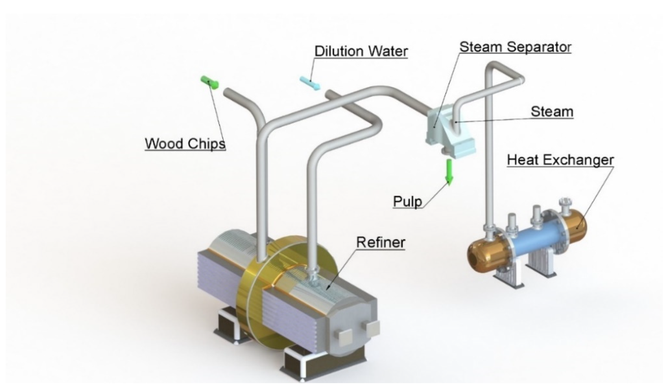
Figure 1. A single-disc refiner connected to the heat recovery unit (studied case).
Energies 13 05113 g001
Figure 2. The structure of the adaptive neuro-fuzzy inference system (ANFIS) method consisting of two rules, two model inputs, one model output.
Energies 13 05113 g002
Figure 3. Single habitat species model.
Energies 13 05113 g003
Figure 4. The main steps for implementing biogeography-based optimization algorithm (BBO) [39].
Energies 13 05113 g004
Figure 5. A schematic diagram of the teaching learning-based optimization algorithm (TLBO) algorithm [41].
Energies 13 05113 g005
Figure 6. Schematic diagram of the particle swarm optimization process.
Energies 13 05113 g006
Figure 7. The design structure of the genetic algorithm.
Energies 13 05113 g007
Figure 8. Structure of ant colony (ACO) optimization algorithm [46].
Energies 13 05113 g008
Figure 9. Differential evolution algorithm flowchart [50].
Energies 13 05113 g009
Figure 10. The structure of the proposed method for refining energy simulation.
Energies 13 05113 g010
Figure 11. (a) creating an initial fuzzy inference system, (b) the function of the particle swarm optimization algorithm (PSO) algorithm for training the ANFIS, and (c) PSO structure.
Energies 13 05113 g011
Figure 12. Histogram of the percentage error of the empirical model used for data validation.
Energies 13 05113 g012
Figure 13. Testing dataset of BBO for predicting motor load (a), and produced steam during the pulp refining process (b).
Energies 13 05113 g013
Figure 14. Test samples of TLBO to estimate motor load (a), and generated steam during the pulp refining process (b).
Energies 13 05113 g014
Figure 15. Test samples of PSO to estimate refining motor load (a), and refining steam generation (b).
Energies 13 05113 g015
Figure 16. Test samples of genetic algorithm (GA) to estimate refining motor load (a), and refining steam generation (b).
Energies 13 05113 g016
Figure 17. Test samples of ACO to estimate refining motor load (a), and refining steam generation (b).
Energies 13 05113 g017
Figure 18. Test samples of differential evolution (DE) to estimate refining motor load (a), and refining steam generation (b).
Energies 13 05113 g018
Figure 19. Comparison of the statistical indicators for six evolutionary algorithms to predict the motor load, (a) RMSE, (b) MSE, and (c) R.
Energies 13 05113 g019
Figure 20. Comparison of the statistical indicators for six evolutionary algorithms to predict the steam generation, (a) RMSE, (b) MSE, and (c) R.
Energies 13 05113 g020
Table 1. Artificial neural network (ANN) model input and target variables.
Refining Plate GapRefining Dilution WaterSite Ambient TemperatureFeeder Screw SpeedRefining Motor LoadRefining Generated Steam
predictor variables
Target variable
Table 2. Data validation analysis for the refiner.
ParameterMeasure
M A P E 0.0460
R 2 0.72
R 0.84
R M S E   ( MW ) 0.35
a 8.655
b 1.719
k m 1.240
Table 3. Model evaluation criteria for six evolutionary algorithms contributing to ANFIS for refining motor load prediction.
Optimization AlgorithmMSE-TrainMSE-TestRMSE-TrainRMSE-TestR-TrainR-Test
TLBO0.12560.12160.35440.34880.83920.8472
BBO0.10460.11180.32350.33440.8590.8511
DE0.11030.11550.33210.33980.85240.840
AC0.11550.11670.33990.34160.84240.843
GA0.089540.094940.299240.308130.88350.8677
PSO0.07050.07350.26550.27120.90680.9052
Table 4. Model evaluation criteria for six evolutionary algorithms contributing to ANFIS to predict the refining steam generation.
Optimization AlgorithmMSE-TrainMSE-TestRMSE-TrainRMSE-TestR-TrainR-Test
TLBO0.02210.02110.14870.14520.84960.8607
BBO0.01740.017570.131940.132560.86890.8682
DE0.017890.016970.13370.13030.86720.871
AC0.019250.018560.13870.13620.85240.8624
GA0.015560.016110.124760.126940.88360.8804
PSO0.01050.01280.10250.11310.9240.9032