Chattering-Free Single-Phase Robustness Sliding Mode Controller for Mismatched Uncertain Interconnected Systems with Unknown Time-Varying Delays

Abstract

Variable structure control with sliding mode can provide good control performance and excellent robustness. Unfortunately, the chattering phenomenon investigated due to discontinuous switching gain restricting their applications. In this paper, a chattering free improved variable structure control (IVSC) for a class of mismatched uncertain interconnected systems with an unknown time-varying delay is proposed. A sliding function is first established to eliminate the reaching phase in traditional variable structure control (TVSC). Next, a new reduced-order sliding mode estimator (ROSME) without time-varying delay is constructed to estimate all unmeasurable state variables of plants. Then, based on the Moore-Penrose inverse approach, a decentralized single-phase robustness sliding mode controller (DSPRSMC) is synthesized, which is independent of time delays. A DSPRSMC solves a complex interconnection problem with an unknown time-varying delay term and drives the system’s trajectories onto a switching surface from the initial time instance. Particularly, by applying the well-known Barbalat’s lemma, the chattering phenomenon in control input is alleviated. Moreover, a sufficient condition is established by using an appropriate Lyapunov theory and linear matrix inequality (LMI) method such that a sliding mode dynamics is asymptotically stable from the beginning time. Finally, a developed method is validated by numerical example with computer simulations.

1. Introduction

In practical control systems, chattering and time delays are common phenomena. These have motivated the study of chattering removal problems and time-delay systems, leading to many useful results [1,2,3,4,5,6,7]. The chattering phenomenon causes reducing of control precision or in the worst-case, drive the system to its resonant [8]. In addition, time delay existence can induce degradation and/or instability in system performance [9,10]. Hence, one of the efficient techniques is the traditional variable structure control (TVSC) theory [11,12,13]. Due to its various attractive features such as quick response, good transient performance, excellent robustness, external disturbances rejection ability, and its insensitivity to uncertainties and parameter variations TVSC has been successfully applied to enhance the stability of the time delay of uncertain systems, as indicated by a large number of quality papers published in the most recent internationally renowned journals and the related references therein [14,15,16,17,18,19].

Based on the advantages of TVSC, the problem of decentralized control design for interconnected systems has attracted significant attention, and several approaches for designing robust state feedback control schemes have been reported [20,21,22,23]. In particular, a robust decentralized sliding mode controller was derived on the basic properties of the Lur’e-Postnikov systems for the interconnected systems with series nonlinearities [21]. By using the well-known closed-loop eigenvalue/eigenvector method, a novel decentralized controller was developed for a class of mismatched uncertain systems [22]. A decentralized robust controller was designed for a class of decentralized multi-input perturbed systems via the multiple-sliding surface [20]. The design problem of robust decentralized adaptive neutral control was investigated for a class of non-affine nonlinear interconnected systems with unknown dead zones and without the uncertainties [23]. Nevertheless, these works did not consider the time delays in the systems, which is important in both theory and real-world applications. Furthermore, the studies assumed that the states of the system are measurable, but in most practical situations, state variables are generally not easy to obtain for many reasons, such as the limitations of available measurement equipment. Therefore, the design problems of a decentralized sliding mode controller (DSMC) based on full order sliding mode estimator (FOSME) and output information using only are necessary for time-delay systems [24,25,26,27,28,29]. An estimator–based DSMC was established for a class of nonlinear interconnected systems with time delays by employing the neural network approximation theory and backstepping design method [24]. Also, following this technique, a decentralized adaptive output feedback controller was presented for a class of time-delay systems with saturating input constraints [28]. An adaptive neural network DSMC based on FOSME was constructed for a class of uncertain nonlinear systems with immeasurable states and unknown time delays [25]. The authors proposed a decentralized adaptive output feedback stabilizer for a class of nonlinear time-delay systems without a priori knowledge of subsystem high-frequency gain signs [26]. A decentralized robust output feedback control scheme was developed by combining the backstepping technique with adaptive fuzzy control theory for a class of strict feedback nonlinear systems [27]. A decentralized fault-tolerant controller was proposed for a class of interconnected nonlinear systems under the Lipschitz condition via the cyclic small gain methodology [29]. However, these studies did not consider the uncertainty in the i–th subsystem. In order to solve this problem, studies [30,31] have proposed a class of time-delay interconnected systems with uncertainty in the state matrix and in interconnections. A DSMC was synthesized to stabilize a class of time-delay systems with nonlinear interconnections by using the Lyapunov-Razumikhin approach [30]. By using the known-well linear matrix inequality (LMI), a DSMC was investigated to be connectively stable with maximized interconnection bounds for a class of interconnected time-delay systems [31]. Unfortunately, limitations of these works to be considered are the uncertainty in the state matrix of system and in interconnections under matching conditions. Recently, there are several interesting studies that focused on the interconnected time-delay systems with mismatched uncertainty in the state matrix or in interconnection such as [14,15,16]. Notably, a FOSME—based decentralized control problem was established by the singular value decomposition approach for a class of interconnected systems of neutral type considering only mismatched uncertainty in the system’s state matrix [14]. A DSMC was proposed based on the Razumikhin–Lyapunov method for a class of interconnected time-delay systems [15]. The problem of decentralized memory static output feedback control design was investigated for a class of nonlinear time-delay interconnected systems with a similar structure under strict Lipschitz constraint [16]. However, the studies [15,16] consider the matched uncertainty in the state matrix and the mismatched uncertainty in interconnections when designing the decentralized output feedback controller under known time delays constraint.

Although the DSMC guarantees robustness for the matched and mismatched uncertain systems with time-varying delays, implementation of the DSMC becomes challenging due to a major disadvantage known as chattering. In the chattering phenomenon, a high-frequency motion makes the state trajectories of the system rapidly oscillating about the sliding surface. It may excite the unmodelled system dynamics and lead to premature wear and tear or even breakdown of the system. In the recent past, a lot of techniques have been investigated to reduce the chattering phenomenon in DSMCs [32,33,34,35]. Among the various solutions to prevent the chattering, the boundary layer [34] is probably the most common method instead of a sign or saturation function [32,33] in order to have a continuous output in the system’s control law. However, the use of this method has two drawbacks. First, when the noise in measurement has a high level, so the effectiveness of the system in boundary layer design is reduced. Second, the finite reaching time from initial states to the switching phase is not ensured when applying the continuous approximation. To solve the problems, the higher-order sliding mode control was investigated for mitigating the chattering in uncertain multi-input and multi-output nonlinear systems [35]. Nevertheless, this technique requires a complex implementation algorithm which is difficult to estimate the high-order derivatives of the system’s states. As a special case of the higher-order sliding mode control, the second-order sliding mode control technique was successfully applied for avoiding the chattering effect with finite-time convergence in the previous works [36,37,38,39]. Recently, a second-order sliding mode controller was designed by combining a proportional-integral term of the sliding variable and an integral sign function term into the control signal [36]. A second-order control scheme was established by using geometric homogeneity and adaptive sliding mode concept [37]. To effectively avoid the chattering, the authors used the low-pass integrator properties in the second-order control input [38]. This algorithm does not need the derivative of the sliding variable; hence, the requirement of designing a differentiator is removed. Thus, the second-order sliding mode control method is easy to implement and less information demand. However, these studies must be assumed to be the second derivative of all state variables that must be existed, even though the mathematical model of systems is the first order. This is not realistic in practice. Another way is to eliminate the chattering that uses a proportional plus integral sliding surface in the controller under a restrictive condition for the bound of the disturbance derivative [39]. Consequently, the presented techniques are still serious in solving the chattering problem. Recently, it was noticed that several researchers introduce new techniques using the well-known Barbalat’s lemma for DSMCs to soothe the chattering problem and keep its control performance [17,18]. However, the methods given in these studies are only available for small scale systems, therefore, they cannot be applied for the complex problem of decentralized control design for interconnected systems with unknown time-varying delay, external disturbance, and mismatched interconnections. As a result, it is the key for decentralized control systems to develop a chattering free improved variable structure control (IVSC) utilizing output signal. The chattering free IVSC is extremely necessary and reaching phase elimination is currently indispensable. In the chattering free IVSC, the sliding mode dynamics of the interconnected system with unknown varying-time delays is asymptotically stable in the zero reaching time.

For the aforementioned reasons, the aim of this paper was the development of a decentralized single-phase robustness sliding mode controller (DSPRSMC) for a class of mismatched uncertain systems with interconnections and unknown time-varying delays via Moore-Penrose inverse approach. The main contributions of this paper are summarized below:

(1)

Propose an IVSC that eliminates the reaching phase by establishing a new sliding function. It enables the plant’s trajectories always start from the initial time instance.

(2)

A DSPRSMC is constructed based on an output signal and the estimated state variables from a reduced-order sliding mode estimator (ROSME). As a result, the robust property of the system is guaranteed and the overall stability of the system is assured.

(3)

The results of existing work [14,15,16,17,18] are extended to a class of interconnected plants with mismatched interconnections and unknown time-varying delays when the reaching phase is eliminated.

(4)

The chattering in control input is alleviated by combining the well-known Barbalat’s lemma and Lyapunov stability theory. Also, computer simulation results are provided to show the feasibility of the proposed scheme as well as to demonstrate the effectiveness of the analytical results.

The outline of this paper is as follows: Section 2 describes the preliminaries of the system, the definition of the sliding function, and the considered problem is formulated, which will be used to find achievements in the next section. Section 3 is the key part in this work including the establishment of ROSME, DSPRSMC design for improving the robustness and performance of the interconnected time-delay system, and mitigating the chattering phenomenon. The stability of the overall system is demonstrated in Section 4 by employing the Lyapunov function and the LMI method. One computer simulation is presented in Section 5 to show the advantages and effectiveness of the developed technique. Finally, conclusions are drawn in Section 6.

The notations that will be used through the paper are standard. $\Vert x(t)\Vert =\sqrt{x^T(t)x(t)}$ denotes the Euclidean norm of a vector and $\Vert A\Vert =\sqrt{{\lambda }_{\max }(A^{T}A)}$ stands for the induced spectral norm of a matrix. $A^T$ and ${\lambda }_{\max }(A)$ are the transpose and maximum eigenvalues of a matrix $A,$ respectively. $A>0$ means that $A$ is real symmetric and positive definite. I and 0 represent the identity matrix and a zero matrix, respectively. $M^{\perp }$ denotes an orthogonal complement of a matrix $M,$ i.e., $M^{\perp T}{M}^{\perp }=I$ and $M{M}^{\perp }=0$ or $M^T{M}^{\perp }=0.$

2. System Descriptions and Problem Formulation

In this section, a general class of the interconnected systems with mismatched uncertainty where are included $L$ subsystems with unknown time-varying delays in the interconnections and external disturbances. The system’s state-space form for each subsystem is described as follows:

$$\begin{array}{ll}{\dot{x}}_i(t)& =\left[A_{ii}+\Delta A_{ii}(t)\right]x_i(t)+B_i\left[u_i(t)+{\varpi }_i(x_i(t),x_i(t-d_i(t)),t)\right]\\ & +{\displaystyle \sum _{\begin{array}{l}j=1\\ j\ne i\end{array}}^L\left[F_{ij}+\Delta F_{ij}{}_{d_j}(t)\right]x_j(t-d_j(t))},\\ y_i(t)=& C_i{x}_i(t),\\ x_i(t)=& {\chi }_i(t),for-{\overline{d}}_i\le t<0,\end{array}$$

(1)

where for the $i^{\mathrm{th}}$ subsystem $x_i\in R^{n_i}$ is the continuous-time state variables of the system, $u_i\in R^{m_i}$ is the control signal, and $y_i\in R^{p_i}$ is measured control output. The character j is the index of interconnection subsystems. The matrices $\Delta A_{ii}(t)=M_{ii}{\Sigma }_{ii}(x_i(t),t)N_{ii}$ and $\Delta F_{ij{d}_j}(t)=$ $D_{ij}{\Sigma }_{ij}(x_i(t),x_i(t-d_j(t)),t)E_{ij}$ show the mismatched uncertainty of the system and mismatched interconnections with unknown time-varying delay in each isolated subsystem, respectively. The matrices ${\Sigma }_{ii}(x_i(t),t)$ and ${\Sigma }_{ij}(x_i(t),x_i(t-d_j(t)),t)$ are unknown functions. The constant matrices $A_{ii},B_i,F_{ij},M_{ii},N_{ii},D_{ij},E_{ij},$ and $C_i$ have known parameters. The term ${\varpi }_i(x_i(t),x_i(t-d_i(t)),t)$ presents the matched disturbances of the plant in the $i^{\mathrm{th}}$ subsystem. The function $d_i(t)$ is the time-varying delay which is assumed to be unknown, non-negative and bounded in ${\Re }^{+},$ that is, ${\overline{d}}_i:={\sup }_{t\in {\Re }^{+}}\left\{d_i(t)\right\}<\infty .$ The character ${\chi }_i(t)$ represents differential vector-valued initial function on $[-{\overline{d}}_i,0].$ The main purpose of this paper is to synthesize a decentralized single-phase robustness sliding mode controller (DSPRSMC) for mismatched uncertain interconnected systems with unknown varying-time delays (Equation (1)) such that the overall of the closed-loop system is asymptotically stable and the chattering in control input is removed. The following is assumed regarding the systems for design the DSPRSMC.

A1:

The matrices $B_i$ and $C_i$ have full rank and $\mathrm{rank}(C_i{B}_i)=m_i.$

A2:

The matched disturbance input satisfies the conditions that there exist nonnegative, but unknown, constants ${\beta }_{1_i}$ and ${\beta }_{1_i}$ such thatfor:

$$\Vert {\varpi }_i(x_i(t),x_i(t-d_i(t)),t)\Vert \le {\beta }_{1_i}+{\beta }_{2_i}\left(\Vert x_i\Vert +\Vert x_i(t-d_i(t))\Vert \right).$$

(2)

A3:

The matrices $\Delta A_{ii}(t)$ and $\Delta F_{ij{d}_j}(t)$ denote the mismatched parameter uncertainties in the state of each isolated subsystem and interconnection elements. We assume that for all $(x_i,t)$ and $(x_j,t)\in R^{n_i}\mathrm{x}R,$

$$\Vert {\Sigma }_{ii}(x_i,t)\Vert \le 1\mathrm{and}\Vert {\Sigma }_{ij}(x_i(t),x_i(t-d_j(t)),t)\Vert \le 1.$$

(3)

Remark 1.

The mathematical model of the system (Equation (1)) is extended from the published studies [15,19,40]. The$\mathrm{rank}(C_i{B}_i)=m_i$in Assumption 1 is a limitation on the triplet$(A_i,B_i,C_i)$and is the existing condition of the output sliding surface. Further, the Assumptions 1–3 are standard assumptions in the existing works of the traditional variable structure control (TVSC) [14,19,41].

Now, we develop a new approach for the design of single-phase to be used in the context of the mismatched uncertain system with unknown time-varying delays for each subsystem. The proposed sliding function is defined as:

$${\sigma }_i(y_i(t),t)={\overline{\sigma }}_i(y_i,t)-{\overline{\sigma }}_i(y_i,0)\exp (-{\alpha }_{i}t),i=1,2,\dots ,L,$$

(4)

where the term ${\overline{\sigma }}_i(y_i,t)=S_i{x}_i=P_i{y}_i$ with $S_i=P_i{C}_i,$ and ${\alpha }_i$ is a positive scalar. In addition, we assume that the sliding matrix $S_i$ must satisfy the following properties:

Property 1:

$(S_i{B}_i)$ is non-singular.

Property 2:

When the reaching phase is eliminated, the states of the plant move into switching surface from the initial time instance. As a result, the reduced-order sliding mode dynamics is asymptotically stable.

Property 3:

Owing to assumption 2 and 3, the sliding mode dynamics must guarantee the invariant property for any uncertainties and external disturbances.

Remark 2.

The equation$S_i=P_i{C}_i$is assumed to be solvable. The sliding surface parameter matrix$S_i$also must satisfy the properties 1–3 where are generally developed from the previous papers [19,42,43].

Remark 3.

In the design of TVSC, the robustness and performance of the system are not ensured in during complete intervals of a control signal. That is, the desired motion of the system has only achieved after the sliding motion has happened. In order to solve the drawback, the switching function is proposed in the Equation (4). From this equation, it is plainly seen that the sliding mode,${\sigma }_i(y_i(t),t)=0,$exists from the beginning time$t=0$and there is no reaching phase which is eliminated. This technique ensures that the system’s state moves into switching surface from the initial time whose the reaching time is equal to zero. This leads to enhancing the robustness of the system which is necessary in sliding mode control design.

To guarantee the properties 1–3, the Moore-Penrose inverse approach is introduced in [42] for designing the DSPRSMC. That is, there are symmetric matrices $R_{1i}\mathrm{and}{R}_{2i}$ exist and satisfy the two following the linear matrix inequalities (LMIs):

$$\begin{array}{c}{\Gamma }_i{R}_{1i}{\Gamma }_i+B_i{R}_{2i}{B}_i^T>0,\\ B_i^{\perp T}\left(A_i{\Gamma }_i{R}_{1i}{\Gamma }_i+{\Gamma }_i{R}_{1i}{\Gamma }_i{A}_i^T\right)B_i^{\perp }<0,\end{array}$$

(5)

where ${\Gamma }_i$ and ${\Gamma }_j$ are $n\mathrm{x}n$ symmetric matrices such that:

$$\begin{array}{l}{\Gamma }_i=I_{i}if{B}_i^{\perp T}{M}_{ii}=0,\\ {\Gamma }_i=I_i-N_{ii}^g{N}_{ii}if{B}_i^{\perp T}{M}_{ii}\ne 0,\end{array}\mathrm{and}\begin{array}{l}{\Gamma }_j=I_{j}if{B}_i^{\perp T}{D}_{ij}=0,\\ {\Gamma }_j=I_j-E_{ij}^g{E}_{ij}if{B}_i^{\perp T}{D}_{ij}\ne 0,\end{array}$$

(6)

where $N_{ii}^g$ and $E_{ij}^g$ are the Moore-Penrose inverse of the matrices $N_{ii}$ and $E_{ij},$ respectively, and $B_i^{\perp }$ is any basis of the null space of the matrix $B_i^T.$

Remark 4.

The term$B_i^{\perp }{M}_{ii}=0$and$B_i^{\perp }{D}_{ij}=0,$that is, the uncertainties of systems and the interconnection are matched. Otherwise, the term$B_i^{\perp }{M}_{ii}\ne 0$and$B_i^{\perp }{D}_{ij}\ne 0,$that is, the uncertainties of systems and the interconnection are mismatched.

The sliding surface matrix guaranteeing properties 1, 2, and 3 are parameterized by:

$$S_i=K_i{B}_i^T{\left({\Gamma }_i{R}_{1_i}{\Gamma }_i+B_i{R}_{2_i}{B}_i^T\right)}^{-1},$$

(7)

where $K_i$ is any $m_i\mathrm{x}{m}_i$ non-singular matrix, and the matrix $H_i={\Gamma }_i{R}_{1_i}{\Gamma }_i+B_i{R}_{2_i}{B}_i^T.$ And the matrix $P_i$ should be selected to satisfy $S_i=P_i{C}_i.$ Now, the transformation matrix ${\mathsf{\Pi }}_i$ is introduced to achieve the regular form from the original uncertain interconnected systems (Equation (1)):

$${\mathsf{\Pi }}_i=\left[\begin{array}{c}{B}_i^{\perp T}\\ K_i{B}_i^T{H}_i^{-1}\end{array}\right],\left[\begin{array}{l}{z}_i\\ {\overline{\sigma }}_i\end{array}\right]={\mathsf{\Pi }}_i{x}_i,$$

(8)

where the dynamic variable $z_i\in R^{n_i-m_i}$ is unmeasurable and the sliding variable ${\overline{\sigma }}_i(y_i,t)\in R^{m_i}$ is measurable. We can see that the inverse form of the matrix ${\mathsf{\Pi }}_i$ is ${\mathsf{\Pi }}_i^{-1}=$ $\left[H_i{B}_i^{\perp }{\left(B_i^{\perp T}{H}_i{B}_i^{\perp }\right)}^{-1}{B}_i{\left(S_i{B}_i\right)}^{-1}\right].$ By employing the above transformation, one can obtain:

$$\begin{array}{ll}\left[\begin{array}{l}{\dot{z}}_i\\ {\dot{\overline{\sigma }}}_i\end{array}\right]=& \left[A_{ii}+\Delta A_{ii}(t)\right]\left[\begin{array}{l}{z}_i(t)\\ {\overline{\sigma }}_i(t)\end{array}\right]{\mathsf{\Pi }}_i^{-1}+B_i\left\{u_i(t)+{\varpi }_i(\left[\begin{array}{l}{z}_i(t)\\ {\overline{\sigma }}_i(t)\end{array}\right]{\mathsf{\Pi }}_i^{-1},\left[\begin{array}{l}{z}_i(t-d_i(t))\\ {\overline{\sigma }}_i(t-d_i(t))\end{array}\right]{\mathsf{\Pi }}_i^{-1},t)\right\}\\ & +{\displaystyle \sum _{\begin{array}{l}j=1\\ j\ne i\end{array}}^L\left[F_{ij}+\Delta F_{ij}{}_{d_j}(t)\right]\left[\begin{array}{l}{z}_j(t-d_j(t))\\ {\overline{\sigma }}_j(t-d_j(t))\end{array}\right]{\mathsf{\Pi }}_j^{-1}}.\end{array}$$

(9)

Also, the above equation can be represented in the regular form as follows:

$$\begin{array}{ll}\left[\begin{array}{l}{\dot{z}}_i(t)\\ {\dot{\overline{\sigma }}}_i(t)\end{array}\right]=& \left[\begin{array}{ll}{\overline{A}}_{ii11}+\Delta {\overline{A}}_{ii11}& {\overline{A}}_{ii12}+\Delta {\overline{A}}_{ii12}\\ {\overline{A}}_{ii21}+\Delta {\overline{A}}_{ii21}& {\overline{A}}_{ii22}+\Delta {\overline{A}}_{ii22}\end{array}\right]\left[\begin{array}{l}{z}_i(t)\\ {\overline{\sigma }}_i(t)\end{array}\right]+\left[\begin{array}{l}0\\ S_i{B}_i\end{array}\right]\left[u_i(t)+{\varpi }_i(x_i(t),x_i(t-d_i(t)),t)\right]\\ & +{\displaystyle \sum _{\begin{array}{l}j=1\\ j\ne i\end{array}}^L\left[\begin{array}{ll}{\overline{F}}_{ij11}+\Delta {\overline{F}}_{ij11d_j}& {\overline{F}}_{ij12}+\Delta {\overline{F}}_{ij12d_j}\\ {\overline{F}}_{ij21}+\Delta {\overline{F}}_{ij21d_j}& {\overline{A}}_{ij22}+\Delta {\overline{F}}_{ij22d_j}\end{array}\right]\left[\begin{array}{l}{z}_j(t-d_j(t)\\ {\overline{\sigma }}_j(t-d_j(t)\end{array}\right]},\end{array}$$

(10)

where:

$$\begin{array}{l}{\overline{A}}_{ii11}+\Delta {\overline{A}}_{ii11}(t)=B_i^{\perp T}\left[A_{ii}+M_{ii}{\Sigma }_{ii}(x_i,t)N_{ii}\right]H_i{B}_i^{\perp }{\left(B_i^{\perp T}{H}_i{B}_i^{\perp }\right)}^{-1},\\ {\overline{A}}_{ii12}+\Delta {\overline{A}}_{ii12}(t)=B_i^{\perp T}\left[A_{ii}+M_{ii}{\Sigma }_{ii}(x_i,t)N_{ii}\right]B_i{\left(S_i{B}_i\right)}^{-1},\\ {\overline{A}}_{ii21}+\Delta {\overline{A}}_{ii21}(t)=K_i{B}_i^T{H}_i^{-1}\left[A_{ii}+M_{ii}{\Sigma }_{ii}(x_i,t)N_{ii}\right]H_i{B}_i^{\perp }{\left(B_i^{\perp T}{H}_i{B}_i^{\perp }\right)}^{-1},\\ {\overline{A}}_{ii22}+\Delta {\overline{A}}_{ii22}(t)=K_i{B}_i^T{H}_i^{-1}\left[A_{ii}+M_{ii}{\Sigma }_{ii}(x_i,t)N_{ii}\right]B_i{\left(S_i{B}_i\right)}^{-1},\\ {\overline{F}}_{ij11}+\Delta {\overline{F}}_{ij11d_j}(t)=B_i^{\perp T}\left[F_{ij}+D_{ij}{\Sigma }_{ij}(x_i(t),x_i(t-d_j(t)),t)E_{ij}\right]H_i{B}_i^{\perp }{\left(B_i^{\perp T}{H}_i{B}_i^{\perp }\right)}^{-1},\\ {\overline{F}}_{ij12}+\Delta {\overline{F}}_{ij12d_j}(t)=B_i^{\perp T}\left[F_{ij}+D_{ij}{\Sigma }_{ij}(x_i(t),x_i(t-d_j(t)),t)E_{ij}\right]B_i{\left(S_i{B}_i\right)}^{-1},\\ {\overline{F}}_{ij21}+\Delta {\overline{F}}_{ij21d_j}(t)=S_i\left[F_{ij}+D_{ij}{\Sigma }_{ij}(x_i(t),x_i(t-d_j(t)),t)E_{ij}\right]H_i{B}_i^{\perp }{\left(B_i^{\perp T}{H}_i{B}_i^{\perp }\right)}^{-1},\\ {\overline{F}}_{ij22}+\Delta {\overline{F}}_{ij22d_j}(t)=S_i\left[F_{ij}+D_{ij}{\Sigma }_{ij}(x_i(t),x_i(t-d_j(t)),t)E_{ij}\right]B_i{\left(S_i{B}_i\right)}^{-1},\\ z_i=B_i^{\perp T}{x}_i,\mathrm{and}{\overline{\sigma }}_i=Py=S_i{x}_i.\end{array}$$

Equation (10) can be rewritten by:

$$\begin{array}{ll}{\dot{z}}_i(t)=& \left({\overline{A}}_{ii11}+\Delta {\overline{A}}_{ii11}\right)z_i(t)+\left({\overline{A}}_{ii12}+\Delta {\overline{A}}_{ii12}\right){\overline{\sigma }}_i(t)\\ & +{\displaystyle \sum _{\begin{array}{l}j=1\\ j\ne i\end{array}}^L\left[\left({\overline{F}}_{ij11}+\Delta {\overline{F}}_{ij11d_j}\right)z_j(t-d_j(t)+\left({\overline{F}}_{ij12}+\Delta {\overline{F}}_{ij12d_j}\right){\overline{\sigma }}_j(t-d_j(t))\right]},\\ {\dot{\overline{\sigma }}}_i(t)=& \left({\overline{A}}_{ii21}+\Delta {\overline{A}}_{ii21}\right)z_i(t)+\left({\overline{A}}_{ii22}+\Delta {\overline{A}}_{ii22}\right){\overline{\sigma }}_i(t)+\left(S_i{B}_i\right)u_i(t)\\ & +\left(S_i{B}_i\right){\varpi }_i(x_i(t),x_i(t-d_i(t)),t)\\ & +{\displaystyle \sum _{\begin{array}{l}j=1\\ j\ne i\end{array}}^L\left[\left({\overline{F}}_{ij21}+\Delta {\overline{F}}_{ij21d_j}\right)z_j(t-d_j(t)+\left({\overline{F}}_{ij22}+\Delta {\overline{F}}_{ij22d_j}\right){\overline{\sigma }}_j(t-d_j(t)\right]}.\end{array}$$

(11)

Now, we only consider the problem in the mismatching condition for the uncertainties of the system’s state matrix and interconnections for interconnected systems. Based on the properties of the Moore-Penrose inverse approach and results in [42], we can easily get:

$$\begin{array}{l}\Delta {\overline{A}}_{ii11}(t)=B_i^{\perp T}{M}_{ii}{\Sigma }_{ii}(x_i,t)N_{ii}{H}_i{B}_i^{\perp }{\left(B_i^{\perp T}{H}_i{B}_i^{\perp }\right)}^{-1}=0,\\ \Delta {\overline{F}}_{ij11d_j}(t)=B_i^{\perp T}{D}_{ij}{\Sigma }_{ij}(x_i(t),x_i(t-d_j(t)),t)E_{ij}{H}_i{B}_i^{\perp }{\left(B_i^{\perp T}{H}_i{B}_i^{\perp }\right)}^{-1}=0,\\ \Delta {\overline{A}}_{ii21}(t)=K_i{B}_i^T{H}_i^{-1}\left[M_{ii}{\Sigma }_{ii}(x_i,t)N_{ii}\right]H_i{B}_i^{\perp }{\left(B_i^{\perp T}{H}_i{B}_i^{\perp }\right)}^{-1}=0,\\ \Delta {\overline{F}}_{ij21d_j}(t)=S_i\left[D_{ij}{\Sigma }_{ij}(x_i(t),x_i(t-d_j(t)),t)E_{ij}\right]H_i{B}_i^{\perp }{\left(B_i^{\perp T}{H}_i{B}_i^{\perp }\right)}^{-1}=0.\end{array}$$

(12)

From Equations (11) and (12), the regular form can be represented by the following:

$$\begin{array}{ll}{\dot{z}}_i(t)=& {\overline{A}}_{ii11}{z}_i(t)+\left({\overline{A}}_{ii12}+\Delta {\overline{A}}_{ii12}\right){\overline{\sigma }}_i(t)\\ & +{\displaystyle \sum _{\begin{array}{l}j=1\\ j\ne i\end{array}}^L\left[{\overline{F}}_{ij11}{z}_j(t-d_j(t)+\left({\overline{F}}_{ij12}+\Delta {\overline{F}}_{ij12d_j}\right){\overline{\sigma }}_j(t-d_j(t)\right]},\\ {\dot{\overline{\sigma }}}_i(t)=& {\overline{A}}_{ii21}{z}_i(t)+\left({\overline{A}}_{ii22}+\Delta {\overline{A}}_{ii22}\right){\overline{\sigma }}_i(t)+\left(S_i{B}_i\right)\left[u_i(t)+{\varpi }_i(x_i(t),x_i(t-d_i(t)),t)\right]\\ & +{\displaystyle \sum _{\begin{array}{l}j=1\\ j\ne i\end{array}}^L\left[{\overline{F}}_{ij21}{z}_j(t-d_j(t)+\left({\overline{F}}_{ij22}+\Delta {\overline{F}}_{ij22d_j}\right){\overline{\sigma }}_j(t-d_j(t)\right]},\end{array}$$

(13)

With the purpose of the controller design, we now design a reduced-order sliding mode estimator (ROSME) without time-varying delays.

3. Main Results

3.1. Design a Novel ROSME for the Interconnected Systems with Time-Varying Delay

In order to design a new decentralized single-phase robustness sliding mode controller (DSPRSMC) for a class of mismatched uncertain interconnected systems with interconnections and unknown time-varying delays, we firstly establish new ROSME without time-varying delay. Then, a controller will be constructed based on the upper bound of the estimator error.

Now, a new ROSME will be proposed to estimate the unmeasurable variables of the systems as follows:

$${\dot{\widehat{z}}}_i(t)={\overline{A}}_{ii11}{\widehat{z}}_i(t)+{\overline{A}}_{ii12}{\overline{\sigma }}_i(t)$$

(14)

where ${\widehat{z}}_i(t)$ is the estimation of variable $z_i(t).$

Remark 5.

The novel ROSME design (Equation (14)) is extended from the conventional Luenberger observer investigated by the authors [44,45]. Different from the full order sliding mode estimators (FOSMEs) [14,24,25,28], the dimension of ROSME, which is established in the Equation (14), is lower. So, our proposed ROSME without time-varying delay guarantees that the robustness of the system is enhanced and the conservatism of the computer process is reduced.

The state estimate ${\widehat{z}}_i(t)$ can converge as far as possible to the original state $z_i(t).$ For this, the estimator error between the estimated state and the true state is defined as $e_i(t)={\widehat{z}}_i(t)-z_i(t).$ The estimation error dynamics of the estimator is constructed by combining the first Equations (13) and (14):

$$\begin{array}{ll}{\dot{e}}_i(t)=& {\overline{A}}_{ii11}{e}_i(t)-\Delta {\overline{A}}_{ii12}{\overline{\sigma }}_i(t)+{\displaystyle \sum _{\begin{array}{l}j=1\\ j\ne i\end{array}}^L\left[{\overline{F}}_{ij11}{e}_j(t-d_j(t))\right]}\\ & -{\displaystyle \sum _{\begin{array}{l}j=1\\ j\ne i\end{array}}^L\left[{\overline{F}}_{ij11}{\widehat{z}}_j(t-d_j(t))+{\overline{F}}_{ij12}{\overline{\sigma }}_j(t-d_j(t))\right]}-{\displaystyle \sum _{\begin{array}{l}j=1\\ j\ne i\end{array}}^L\left[\Delta {\overline{F}}_{ij12d_j}{\overline{\sigma }}_j(t-d_j(t))\right]}.\end{array}$$

(15)

Then, by using (Equation(15)) and properties:

$$\begin{array}{c}{\displaystyle \sum _{\begin{array}{l}j=1\\ j\ne i\end{array}}^L\left[{\overline{F}}_{ij11}{e}_j(t-d_j(t))\right]}={\displaystyle \sum _{\begin{array}{l}j=1\\ j\ne i\end{array}}^L\left[{\overline{F}}_{ji11}{e}_i(t-d_i(t))\right]},\\ {\displaystyle \sum _{\begin{array}{l}j=1\\ j\ne i\end{array}}^L\left[{\overline{F}}_{ij11}{\widehat{z}}_j(t-d_j(t))+{\overline{F}}_{ij12}{\overline{\sigma }}_j(t-d_j(t))\right]}={\displaystyle \sum _{\begin{array}{l}j=1\\ j\ne i\end{array}}^L\left[{\overline{F}}_{ji11}{\widehat{z}}_i(t-d_i(t))+{\overline{F}}_{ji12}{\overline{\sigma }}_i(t-d_i(t))\right]},\\ {\displaystyle \sum _{\begin{array}{l}j=1\\ j\ne i\end{array}}^L\left[\Delta {\overline{F}}_{ij12d_j}{\overline{\sigma }}_j(t-d_j(t))\right]}={\displaystyle \sum _{\begin{array}{l}j=1\\ j\ne i\end{array}}^L\left[\Delta {\overline{F}}_{ji12d_i}{\overline{\sigma }}_i(t-d_i(t))\right]},\end{array}$$

(16)

it generates:

$$\begin{array}{ll}{\dot{e}}_i(t)=& {\overline{A}}_{ii11}{e}_i(t)-\Delta {\overline{A}}_{ii12}{\overline{\sigma }}_i(t)+{\displaystyle \sum _{\begin{array}{l}j=1\\ j\ne i\end{array}}^L\left[{\overline{F}}_{ji11}{e}_i(t-d_i(t))\right]}\\ & -{\displaystyle \sum _{\begin{array}{l}j=1\\ j\ne i\end{array}}^L\left[{\overline{F}}_{ji11}{\widehat{z}}_i(t-d_i(t))+{\overline{F}}_{ji12}{\overline{\sigma }}_i(t-d_i(t))\right]}-{\displaystyle \sum _{\begin{array}{l}j=1\\ j\ne i\end{array}}^L\left[\Delta {\overline{F}}_{ji12d_i}{\overline{\sigma }}_i(t-d_i(t))\right]}.\end{array}$$

(17)

To find the upper bound of the estimation error and support the controller design, the matrix ${\overline{A}}_{ii11}$ will be proved to be a stability matrix via the following lemma.

Lemma 1.

Let${\lambda }_{{\max }_i}$is a maximum eigenvalue of the matrix${\overline{A}}_{ii11}$and the matrix${\overline{A}}_{ii11}$is a stable matrix. Then the following statement holds

$$\Vert \exp \left({\overline{A}}_{ii11}t\right)\Vert \le {\gamma }_i\exp \left({\lambda }_{{\max }_i}t\right),$$

(18)

where${\overline{A}}_{ii11}=B_i^{\perp T}{A}_{ii}{H}_i{B}_i^{\perp }{\left(B_i^{\perp T}{H}_i{B}_i^{\perp }\right)}^{-1}$and${\gamma }_i>0.$

Proof of the Lemma 1.

The matrix ${\overline{A}}_{ii11}$ is stable if and only if there exists a positive-definite Lyapunov matrix ${\tilde{H}}_i$ such that:

$${\overline{A}}_{ii11}{\tilde{H}}_i+{\tilde{H}}_i{\overline{A}}_{ii11}^T<0.$$

(19)

Obviously, when the constraint condition (Equation (5)) is feasible, the following inequalities are valid:

$$\begin{array}{l}{H}_i={\Gamma }_i{R}_{1_i}{\Gamma }_i+B_i{R}_{2_i}{B}_i^T>0,\\ B_i^{\perp T}{H}_i{B}_i^T=B_i^{\perp T}{\Gamma }_i{R}_{1i}{\Gamma }_i{B}_i^T>0.\end{array}$$

(20)

The LMI condition (Equation (5)) and (Equation (20)) imply that the previous Lyapunov inequality (Equation (19)) satisfies the expression ${\tilde{H}}_i=B_i^{\perp T}{H}_i{B}_i^{\perp }>0.$ This means that the matrix ${\overline{A}}_{ii11}$ is a stable matrix and its maximum eigenvalues ${\lambda }_{{\max }_i}$ are all negative and real. As a result, we easily obtain the above statement (Equation (18)) for some positive scalars ${\gamma }_i.$ □

Remark 6.

Based on the obtained results of the Lemma 1, the matrix${\overline{A}}_{ii11}$is stable. Consequently, the ROSME (Equation (14)) is asymptotically stable in the sliding mode,${\overline{\sigma }}_i(t)={\overline{\sigma }}_i(t-d_i(t))=0,$which means that${\widehat{z}}_i(t-d_i(t))$in the Equation (17) also converges to zero. Thus, once we can see that the ROSME (Equation (14)) and estimator error dynamics (Equation (17)) are asymptotically stable in sliding mode.

In the following theorem, we will find the upper bound of estimation error that helps the controller design.

Theorem 1.

The matrix${\overline{A}}_{ii11}$is stable, the norm of estimation error in the error dynamics (Equation (17)) is bounded by an upper bound variable${\theta }_i(t)$for all time. The term${\theta }_i(t)$is the solution of:

$$\begin{array}{ll}{\dot{\theta }}_i(t)=& {\lambda }_i{\theta }_i(t)+{\mu }_i{\gamma }_i[{\displaystyle \sum _{\begin{array}{l}j=1\\ j\ne i\end{array}}^L\left({\mu }_{2_j}\Vert {\overline{F}}_{ji11}\Vert \Vert {\widehat{z}}_i(t)\Vert \right)}+\Vert B_i^{\perp T}{M}_{ii}\Vert \Vert N_{ii}{B}_i{\left(S_i{B}_i\right)}^{-1}\Vert \Vert {\overline{\sigma }}_i(t)\Vert \\ & +{\displaystyle \sum _{\begin{array}{l}j=1\\ j\ne i\end{array}}^L{\mu }_{1_j}\left(\Vert {\overline{F}}_{ji12}\Vert +\Vert B_j^{\perp T}{D}_{ji}\Vert \Vert E_{ji}{B}_j{\left(S_j{B}_j\right)}^{-1}\Vert \right)\Vert {\overline{\sigma }}_i(t)\Vert }],\end{array}$$

(21)

where${\lambda }_i={\lambda }_{{\max }_i}+{\mu }_i{\gamma }_i\Vert {\overline{F}}_{ij11}\Vert <0,$${\lambda }_{{\max }_i}$is a maximum eigenvalue of the matrix${\overline{A}}_{ii11}$, the symbols${\gamma }_i,{\mu }_i,{\mu }_{1_j},$and${\mu }_{2_j}$are positive scalars. In addition,${\theta }_i(0)\ge {\gamma }_i\Vert e_i(0)\Vert ,$where${\theta }_i(0)$and$e_i(0)$are the initial conditions of the upper bound variable${\theta }_i(t)$and the error$e_i(t),$ respectively.

The detailed proof of this theorem can be found in Appendix A.

Remark 7.

By solving the Equation (21) via the MATLAB computing environment, we will get the upper bound of estimator error (Equation (17)). A suitable controller will be designed to achieve the objective of this paper, which will be discussed in the next section.

3.2. Construct a DSPRSMC for Reducing the Chattering Phenomenon

In this section, we will propose a DSPRSMC that can render the closed-loop system stable in the sense of mismatched interconnection and external disturbance.

Theorem 2.

For the interconnected systems with unknown time-varying delays (Equation (1)) satisfying assumptions 1–3, if the following constant control gains:

$$\begin{array}{ll}{\rho }_{1_i}=& \Vert {\overline{A}}_{ii21}\Vert +\Vert K_i{B}_i^T{H}_i^{-1}{M}_{ii}\Vert \Vert N_{ii}{H}_i{B}_i^{\perp }{\left(B_i^{\perp T}{H}_i{B}_i^{\perp }\right)}^{-1}\Vert +{\beta }_{2_i}\Vert S_i{B}_i\Vert \\ & \times \left[\Vert H_i{B}_i^{\perp }{\left(B_i^{\perp T}{H}_i{B}_i^{\perp }\right)}^{-1}\Vert +{\epsilon }_i\Vert H_i{B}_i^{\perp }{\left(B_i^{\perp T}{H}_i{B}_i^{\perp }\right)}^{-1}\Vert \right]\\ & +{\displaystyle \sum _{\begin{array}{l}j=1\\ j\ne i\end{array}}^L{\epsilon }_i\left(\Vert {\overline{F}}_{ji21}\Vert +\Vert S_j{D}_{ji}\Vert \Vert E_{ji}{H}_j{B}_j^{\perp }{\left(B_j^{\perp T}{H}_j{B}_j^{\perp }\right)}^{-1}\Vert \right)},\\ {\rho }_{2_i}=& \Vert {\overline{A}}_{ii22}\Vert +\Vert K_i{B}_i^T{H}_i^{-1}{M}_{ii}\Vert \Vert N_{ii}{B}_i{\left(S_i{B}_i\right)}^{-1}\Vert +{\beta }_{2_i}\Vert S_i{B}_i\Vert \left[\Vert B_i{\left(S_i{B}_i\right)}^{-1}\Vert +{\mu }_{1_i}\Vert B_i{\left(S_i{B}_i\right)}^{-1}\Vert \right]\\ & +{\displaystyle \sum _{\begin{array}{l}j=1\\ j\ne i\end{array}}^L{\mu }_{1_j}\left(\Vert {\overline{F}}_{ji22}\Vert +\Vert S_j{D}_{ji}\Vert \Vert E_{ji}{B}_j{\left(S_j{B}_j\right)}^{-1}\Vert \right)},\end{array}$$

(22)

are satisfied, then the control signal:

$$\begin{array}{ll}{u}_i(t)=& -{\eta }_i{\left(S_i{B}_i\right)}^{-1}{\sigma }_i(t)-{\left(S_i{B}_i\right)}^{-1}\{{\rho }_{1_i}\left[\Vert {\widehat{z}}_i(t)\Vert +{\theta }_i(t)\right]+{\rho }_{2_i}\Vert {\overline{\sigma }}_i(t)\Vert \\ & +{\beta }_{1_i}\Vert S_i{B}_i\Vert +{\alpha }_i\Vert P_i\Vert \Vert y_i(0)\Vert \exp (-{\alpha }_{i}t)\}\frac{{\sigma }_i(t)}{\Vert {\sigma }_i(t)\Vert },\end{array}$$

(23)

will render the closed-loop system asymptotically stable.

The Proof of Theorem 2 can be seen in Appendix B.

Remark 8.

A key feature of the proposed improved variable structure control (IVSC) is that the switching function (Equation (4)) and the DSPRSMC (Equation (23)) are designed to be dependent on only output information and estimated variables from the ROSME (Equation (14)). This controller ensures that the state trajectories at arbitrary initial value will hit the sliding surface from very beginning time and the original system (Equation (1)) is asymptotically stable in sliding mode. Thus, the obtained results solved the limitations imposed in the design of the existing works [20,21,22,23,29].

Remark 9.

However,${\sigma }_i(t)/\Vert {\sigma }_i(t)\Vert$in overall control$u_i(t)$(Equation (23)) will cause the control input to produce the chattering phenomenon which will be happened from the beginning time. This also is the drawback of this method. In order to handle this disadvantage, we will establish the following theorem which will reduce the chattering in control input.

Theorem 3.

Suppose that the external perturbations and mismatched uncertainties of the interconnected systems (Equation (1)) with unknown time-varying delays satisfy the assumptions 1–3. Let the control signal be:

$${\overline{u}}_i(t)=-{\left(S_i{B}_i\right)}^{-1}\left\{{\overline{\rho }}_{1_i}\left[\Vert {\widehat{z}}_i(t)\Vert +{\theta }_i(t)\right]\frac{{\sigma }_i}{\Vert {\sigma }_i\Vert }+{\eta }_i{\sigma }_i+{\overline{\rho }}_{2_i}\frac{\Vert {\mathsf{\Theta }}_i\Vert }{\Vert {\mathsf{\Theta }}_i\Vert +{\widehat{\gamma }}_i{e}^{-v_{i}t}}\right\},$$

(24)

where:

$$\begin{array}{l}\begin{array}{ll}{\overline{\rho }}_{1_i}={\rho }_{1_i}=& \Vert {\overline{A}}_{ii21}\Vert +\Vert K_i{B}_i^T{H}_i^{-1}{M}_{ii}\Vert \Vert N_{ii}{H}_i{B}_i^{\perp }{\left(B_i^{\perp T}{H}_i{B}_i^{\perp }\right)}^{-1}\Vert +{\beta }_{2_i}\Vert S_i{B}_i\Vert \\ & \times \left[\Vert H_i{B}_i^{\perp }{\left(B_i^{\perp T}{H}_i{B}_i^{\perp }\right)}^{-1}\Vert +{\epsilon }_i\Vert H_i{B}_i^{\perp }{\left(B_i^{\perp T}{H}_i{B}_i^{\perp }\right)}^{-1}\Vert \right]\\ & +{\displaystyle \sum _{\begin{array}{l}j=1\\ j\ne i\end{array}}^L{\epsilon }_i\left(\Vert {\overline{F}}_{ji21}\Vert +\Vert S_j{D}_{ji}\Vert \Vert E_{ji}{H}_j{B}_j^{\perp }{\left(B_j^{\perp T}{H}_j{B}_j^{\perp }\right)}^{-1}\Vert \right)},\end{array}\\ \begin{array}{l}{\overline{\rho }}_{2_i}={\rho }_{2_i}\Vert {\overline{\sigma }}_i(t)\Vert +{\beta }_{1_i}\Vert S_i{B}_i\Vert +{\alpha }_i\Vert P_i\Vert \Vert y_i(0)\Vert \exp (-{\alpha }_{i}t),\\ \mathrm{and}{\mathsf{\Theta }}_i={\overline{\rho }}_{2_i}\frac{{\sigma }_i}{\Vert {\sigma }_i\Vert }.\end{array}\end{array}$$

(25)

Then the state trajectories of the systems will reach the sliding surface${\sigma }_i(y_i(t),t)=0$from the initial time instance.

The detailed proof of Theorem 3 can be found in Appendix C.

Remark 10.

There are many approaches for reducing the chattering phenomenon such as using a sign or tanh function [32,33], the boundary layer method [34]. However, these approaches affect the accuracy and robustness of the system. In this section, by using the Barbalat’s lemma, the proposed chattering free single-phase sliding mode controller (Equation (24)) offers the major advantage that the chattering in control input is completely rejected, the system’s state trajectories always start from the sliding surface, and the robustness of the system is ensured. Therefore, the designed controller (Equation (24)) is very worthwhile and more realistic, since it can be implemented in many practical control systems.

Remark 11.

For instances, the sign function was used to reduce the chattering for the proton exchange membrane fuel cell [7], the chattering was reduced by using the saturation function in wind energy conversion system [6], and layer boundary method was utilized to handle the high-frequency oscillation in sliding mode controller for a photovoltaic inverter connected to the power grid [5], etc. However, these methods may remove the chattering phenomenon but they have challenges in presence of uncertainty and external disturbances. Consequently, the proposed sliding mode controller (Equation (24)), which is based on the well-known Barbalat’s lemma, can be considered to deal with the chattering phenomenon in these applications.

Remark 12.

The problem of decentralized control design for the matched and mismatched uncertain interconnected systems has a lot of engrossment. In recent years, the published researches about decentralized control remarkably arise from the control of interconnected uncertain systems including hydraulic systems, rolling mills, robotic manipulators, nuclear reactors, manufacturing processes and long transmission lines in pneumatic systems, etc. [1,2,3,4]. In addition, our proposed DSPRSMC can apply to many practical control applications such as flywheel energy storage system [46], grid-connected voltage-source converter [47], synchronous generator [48], photovoltaic–wind interconnected microgrid system [49], and buck boost converter [50].

4. Asymptotically Stable Conditions by LMI Theory

In the above section, the single-phase output feedback controller has been proposed, which is reduced the chattering for interconnected systems with unknown time-varying delays. In this section, the stability of the overall systems will be proved by combining the well-known Lyapunov function and Schur complement formula.

Theorem 4.

Consider the mismatched uncertain interconnected systems (Equation (1)) with assumptions 1–3, and the sliding surface${\sigma }_i(y_i(t),t)=0.$If there exist symmetric matrix${\Xi }_i>0,$and scalars${\phi }_i>0,{\epsilon }_i>0$satisfying:

$$\left[\begin{array}{ccc}{\Psi }_i& {\Xi }_i{\tilde{M}}_i& {\tilde{N}}_i^T\\ {\tilde{M}}_i^T{\Xi }_i^T& -{\phi }_i{I}_i& 0\\ {\tilde{N}}_i& 0& -{\phi }_i^{-1}{I}_i\end{array}\right]<0,$$

(26)

where${\Psi }_i={\overline{A}}_{ii11}^T{\Xi }_i+{\Xi }_i{\overline{A}}_{ii11}+{\displaystyle \sum _{\begin{array}{l}j=1\\ j\ne i\end{array}}^L\left({\epsilon }_i{\overline{F}}_{ji11}^T{\Xi }_i+{\epsilon }_i{\Xi }_i{\overline{F}}_{ji11}+{\phi }_i^{-1}{\epsilon }_i{\Xi }_i{\tilde{D}}_{ji}{\tilde{D}}_{ji}^T{\Xi }_i^T+{\phi }_i{\epsilon }_i{\tilde{E}}_{ji}^T{\tilde{E}}_{ji}\right)}$, then the resulting$(n_i-m_i)$reduced-order dynamics of the time delay systems (Equation (13)) to the sliding surface is asymptotically stable.

Please refer to the detailed proof of this theorem in Appendix D.

Remark 13.

Based on some benefits of the LMI technique [51] over traditional approach methods, the asymptotically stable condition of the overall systems has been established as (Equation (26)). Compared with the recently LMI methods [15,41], the LMI (Equation (26)) shows less conservative results and easily implements by using the LMI Toolbox [52] in MATLAB software.

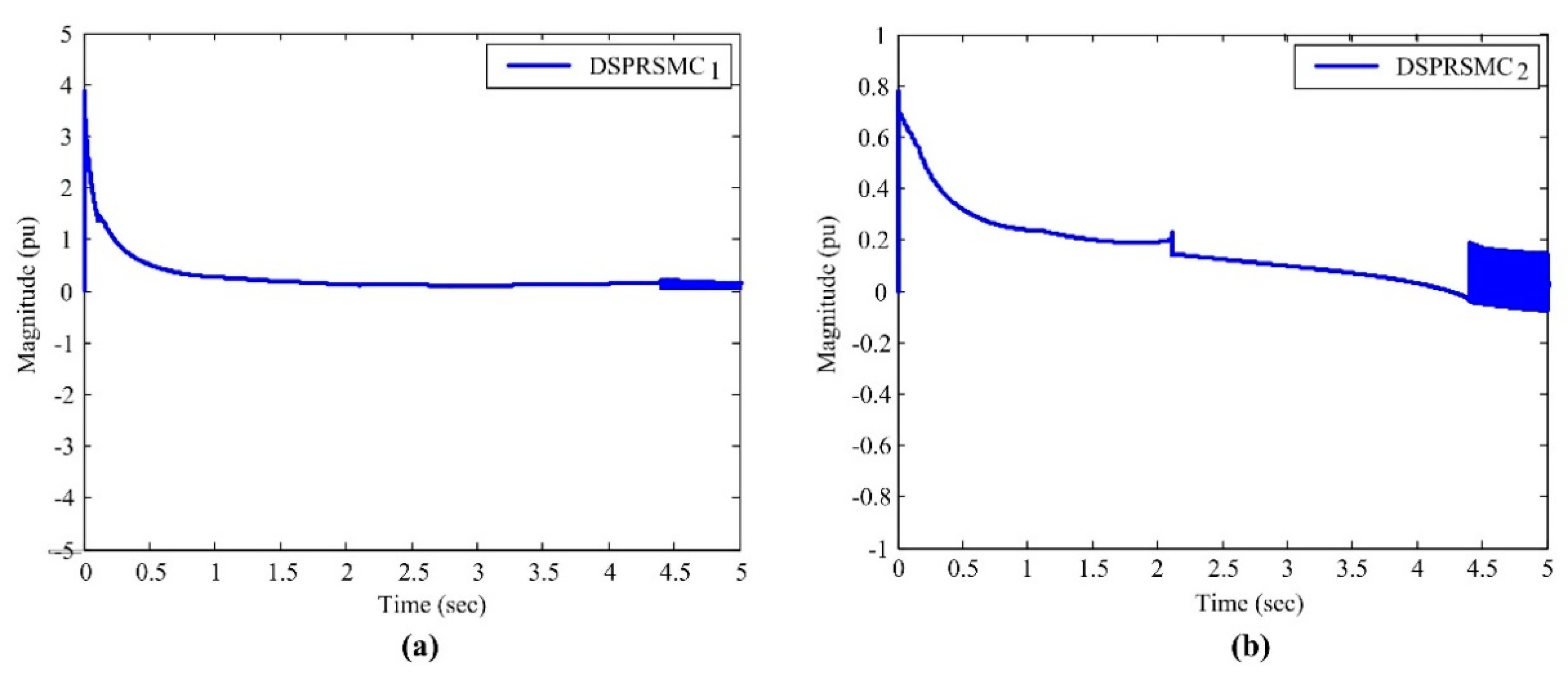
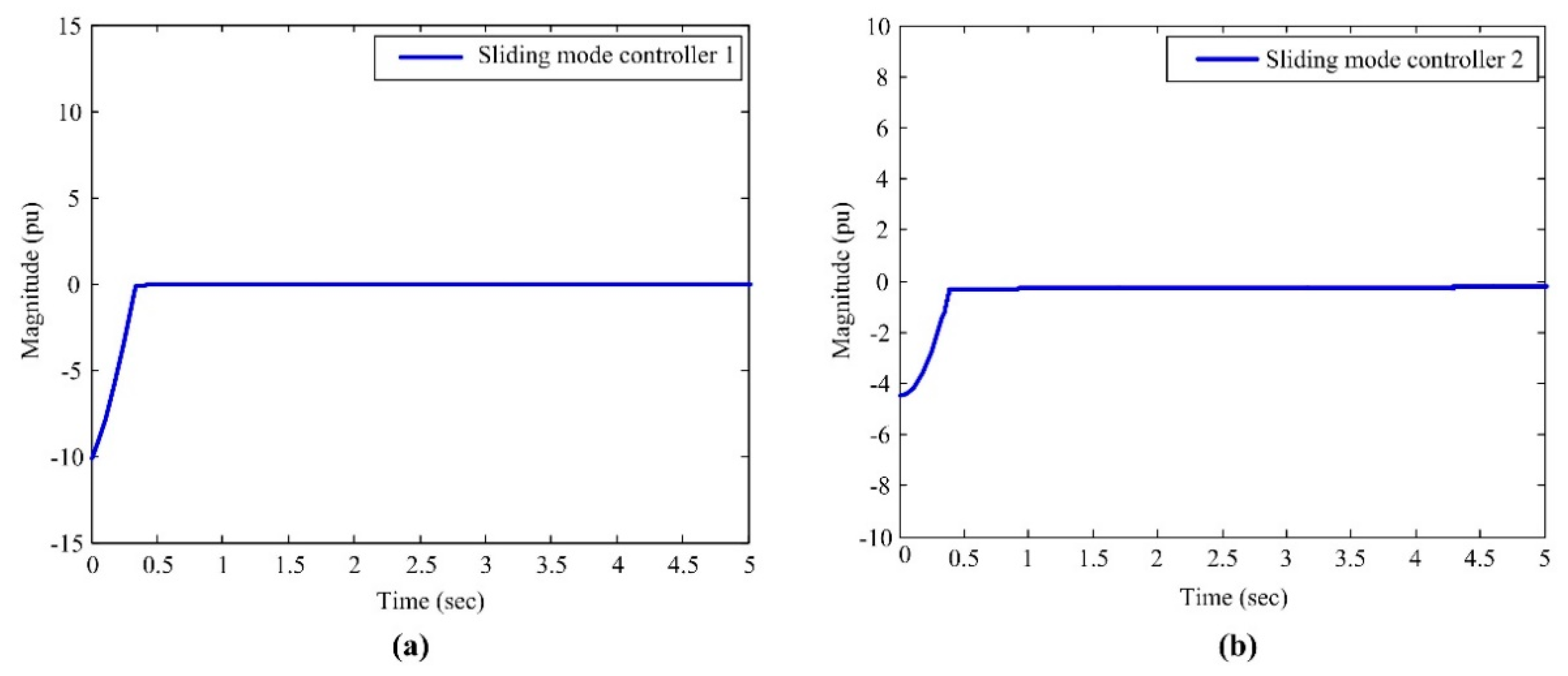
5. Numerical Simulation

To illustrate the proposed method effectiveness, we consider an interconnected time-varying delay system composed of two subsystems model, taken from [53] with some changes, respectively: Subsystem I: $n_1=3,m_1=2,i=1,j=2,$ and the dynamics are given as:

$$\begin{array}{l}{\dot{x}}_1=\left[A_{11}+\Delta A_{11}(t)\right]x_1+B_1\left[u_1(t)+{\varpi }_1(x_1(t),x_1(t-d_1(t)),t)\right]+\left[F_{12}+\Delta F_{12}{}_{d_2}(t)\right]x_2(t-d_2(t))\\ y_1=C_1{x}_1,\end{array}$$

(27)

where $A_{11}=\left[\begin{array}{ccc}-1& 1& 0\\ 0& 1& -1\\ -1& 1& -0.75\end{array}\right],B_1=\left[\begin{array}{l}0\\ 1\\ 0\end{array}\right],C_1=\left[\begin{array}{ccc}1& 1& -1\\ 0& 0& 1\end{array}\right],$ and $F_{12}=\left[\begin{array}{ccc}-0.2& 0& -0.1\\ 0.1& 0& 0\\ 0.2& 0.1& 0\end{array}\right].$ The external disturbances input is $\Vert {\varpi }_1(x_1(t),x_1(t-d_1(t)),t)\Vert \le {\beta }_{2_1}\left(\Vert x_1\Vert +\Vert x_1(t-d_1(t))\Vert \right)$ with ${\beta }_{2_1}=0.22,$ and the mismatched uncertainties in state matrix are $M_{11}{\Sigma }_{11}(x_1,t)N_{11}$ with $M_{11}={\left[001\right]}^T,N_{11}=\left[1\hspace{1em}1\hspace{1em}0\right],$ ${\Sigma }_{11}(x_1,t)=0.14\sin \left(0.1t\right)$ and in interconnections are $D_{12}{\Sigma }_{12}(x_1(t),x_1(t-d_2(t)),t)E_{12}$ with $D_{12}={\left[001\right]}^T,E_{12}=\left[1\hspace{1em}1\hspace{1em}0\right],$ and ${\Sigma }_{12}(x_1(t),x_1(t-d_2(t)),t)=0.23\sin \left(0.1t\right).$

Subsystem II: $n_2=3,m_2=2,i=2,j=1,$ and the dynamics are given as:

$$\begin{array}{l}{\dot{x}}_2=\left[A_{22}+\Delta A_{22}(t)\right]x_2+B_2\left[u_2(t)+{\varpi }_2(x_2(t),x_2(t-d_2(t)),t)\right]+\left[F_{21}+\Delta F_{21}{}_{d_1}(t)\right]x_1(t-d_1(t))\\ y_2=C_2{x}_2,\end{array}$$

(28)

where $A_{22}=\left[\begin{array}{lll}-0.1& 1& 0.2\\ 1& 1& -1\\ 0.5& 1& 0.1\end{array}\right],B_2=\left[\begin{array}{c}0\\ 1\\ -0.5\end{array}\right],C_2=\left[\begin{array}{lll}1& 1& 0\\ 0& 0& 1\end{array}\right],$ and $F_{21}=\left[\begin{array}{ccc}-0.2& 0& -0.1\\ 0.1& 0& 0\\ 0.2& 0.1& 0\end{array}\right].$ The external disturbances input is $\Vert {\varpi }_2(x_2(t),x_2(t-d_2(t)),t)\Vert \le {\beta }_{2_2}\left(\Vert x_2\Vert +\Vert x_2(t-d_2(t))\Vert \right)$ with ${\beta }_{2_2}=0.21,$ and the mismatched uncertainties in state matrix are $M_{22}\Delta {\Sigma }_{22}(x_2,t)N_{22}$ with $M_{22}={\left[100\right]}^T,$ $N_{22}=\left[1\hspace{1em}1\hspace{1em}0\right],$ ${\Sigma }_{22}(x_2,t)=0.12\sin \left(0.1t\right)$ and in interconnections are $D_{21}{\Sigma }_{21}(x_2(t),x_2(t-d_1(t)),t)E_{21}$ with $D_{21}={\left[100\right]}^T,E_{21}=\left[1\hspace{1em}1\hspace{1em}0\right],$ and ${\Sigma }_{21}(x_2(t),x_2(t-d_2(t)),t)=0.24\sin \left(0.3t\right).$

The related parameters required for the simulation are selected as ${\eta }_1=0.011,{\eta }_2=0.021,$ ${\beta }_{1_1}=1.015,{\beta }_{1_2}=1.023,$ ${\beta }_{2_1}=0.25,{\beta }_{2_2}=0.343,$ ${\alpha }_1=1.012,$ ${\alpha }_2=1.017,$ ${\epsilon }_1=1.011,$ ${\epsilon }_2=1.016,$ ${\widehat{\gamma }}_1={\widehat{\gamma }}_2=34.023,$${\nu }_1={\nu }_2=0.042,$ and ${\mu }_{1_1}={\mu }_{1_2}=1.02.$ For simulation, the initial values of two subsystems are $x_1(0)=x_2(0)={[0.01;-0.01;0.02]}^T.$ In addition, let the unknown time-varying delay be $d_1(t)=d_2(t)=0.15\left(1+\sin 0.5t\right)$ [19].

Now, by using the LMI control Toolbox of MATLAB (R2014a, MathWorks, Torrance, CA, USA), the LMI constraints (Equation (5)) are solved to find the following the matrices for two subsystems:

$$\begin{array}{l}{R}_{11}=\left[\begin{array}{lll}103.8211& 43.3650& -6.5634\\ 43.3650& -15.8873& -6.2240\\ -6.5634& -6.2240& 1.2763\end{array}\right],\\ R_{21}=0.9509,\end{array}$$

(29)

and:

$$\begin{array}{c}{R}_{12}=\left[\begin{array}{lll}197.7259& 132.5157& -149.3973\\ 132.5157& 69.4260& -149.5495\\ -149.3973& -149.5495& 1.4154\end{array}\right],\\ R_{22}=0.3796.\end{array}$$

(30)

By solving the Equation (7) through the results (Equation (29)), (Equation (30)), and choose the non-singular matrix $K_1=K_2=I$, the switching surface (Equation (4)) for each subsystem at the initial time $t=0$ are:

$${\sigma }_1(y_1(t),t)=[1.0516\hspace{1em}1.0516]y_1-[1.0516\hspace{1em}1.0516]y_1{e}^{-1.012t}=0$$

(31)

and:

$${\sigma }_2(y_2(t),t)=[2.6344\hspace{1em}0]y_2-[2.6344\hspace{1em}0]y_2{e}^{-1.017t}=0.$$

(32)

Based on the Equation (14), the novel reduced-order sliding mode estimators (ROSMEs) for subsystem I and subsystem II are respectively described by:

$${\dot{\widehat{z}}}_1(t)=\left[\begin{array}{ll}-2.0000& -0.0000\\ 2.0000& -0.7500\end{array}\right]{\widehat{z}}_1(t)+\left[\begin{array}{r}-0.9509\\ 0.9509\end{array}\right]{\overline{\sigma }}_1(t)$$

(33)

and:

$${\dot{\widehat{z}}}_2(t)=\left[\begin{array}{ll}-0.7190& -0.0641\\ 0.7856& -0.6810\end{array}\right]{\widehat{z}}_2(t)+\left[\begin{array}{l}-0.0474\\ 0.6690\end{array}\right]{\overline{\sigma }}_2(t).$$

(34)

In addition, the upper bounds of estimation errors for each subsystem are displayed as:

$${\dot{\theta }}_1(t)=-0.5086{\theta }_1(t)+0.3009\Vert {\widehat{z}}_1(t)\Vert +1.3694\Vert {\overline{\sigma }}_1(t)\Vert$$

(35)

and:

$${\dot{\theta }}_2(t)=-0.3991{\theta }_2(t)+0.2414\Vert {\widehat{z}}_2(t)\Vert +1.4618\Vert {\overline{\sigma }}_2(t)\Vert .$$

(36)

Finally, according to the Theorems 2 and 3, the single-phase sliding mode control laws of subsystems with or without the chattering is shown, respectively:

$$\begin{array}{ll}{u}_1(t)=& -0.9509{\sigma }_1(t)-\{4.4794\left[\Vert {\widehat{z}}_1(t)\Vert +{\theta }_1(t)\right]+3.4708\Vert {\overline{\sigma }}_1(t)\Vert \\ & +1.0000+1.9999\exp (-1.012t)\}\frac{{\sigma }_1(t)}{\Vert {\sigma }_1(t)\Vert },\end{array}$$

(37)

$${\overline{u}}_1(t)=-4.4794\left[\Vert {\widehat{z}}_1(t)\Vert +{\theta }_1(t)\right]\frac{{\sigma }_1}{\Vert {\sigma }_1\Vert }-0.9509{\sigma }_1-{\overline{\rho }}_{2_1}\frac{0.9509\Vert {\mathsf{\Theta }}_1\Vert }{\Vert {\mathsf{\Theta }}_1\Vert +34.023e^{-0.042t}},$$

(38)

and:

$$\begin{array}{ll}{u}_2(t)=& -0.9509{\sigma }_2(t)-\{6.1005\left[\Vert {\widehat{z}}_2(t)\Vert +{\theta }_2(t)\right]+3.6583\Vert {\overline{\sigma }}_2(t)\Vert \\ & +2.5050+2.5051\exp (-1.017t)\}\frac{{\sigma }_2(t)}{\Vert {\sigma }_2(t)\Vert },\end{array}$$

(39)

$${\overline{u}}_2(t)=-\{2.4353\left[\Vert {\widehat{z}}_2(t)\Vert +{\theta }_2(t)\right]\frac{{\sigma }_2}{\Vert {\sigma }_2\Vert }+0.3796{\sigma }_2+{\overline{\rho }}_{2_2}\frac{0.3796\Vert {\mathsf{\Theta }}_2\Vert }{\Vert {\mathsf{\Theta }}_2\Vert +34.023e^{-0.042t}}\},$$

(40)

where ${\widehat{z}}_1(t),{\theta }_1(t)$ and ${\widehat{z}}_2(t),{\theta }_2(t)$ are solutions of the Equations (33)–(36) respectively. The constant control gains ${\overline{\rho }}_{2_1}=3.6500\Vert {\overline{\sigma }}_1(t)\Vert +1.0516+2.1032\exp (-1.012t)$ and ${\overline{\rho }}_{2_2}=3.8472\Vert {\overline{\sigma }}_2(t)\Vert +2.6344+2.6792\exp (-1.017t)$ are used in the controllers (Equation (38)), (Equation (40)), for each subsystem, respectively. The obtained results from the computer simulation are displayed in Figure 1, Figure 2, Figure 3, Figure 4, Figure 5 and Figure 6.

Remark 14.

Figure 1 and Figure 2 are displayed the state trajectories of two subsystems. Figure 1a,b shows the state variables$x_{11}$(solid),$x_{12}$(dashed), and$x_{13}$(dotted) of the first subsystems and state variables$x_{21}$(solid),$x_{22}$(dashed), and$x_{23}$(dotted) of second subsystem corresponding to the controllers$u_1(t)$(Equation (37)) and$u_2(t)$(Equation (39)), respectively. Figure 2a,b presents the state variables$x_{11}$,$x_{12}$, and$x_{13}$of subsystem I and state variables$x_{21}$,$x_{22}$, and$x_{23}$of subsystem II for the controllers${\overline{u}}_1(t)$(Equation (38)) and${\overline{u}}_2(t)$(Equation (40)), respectively. The initial conditions are the same for simulation when the proposed technique is utilized. From these figures, we can see that the state variables for each subsystem are convergent to almost zero quickly. Thus, the proposed ROSME—based the decentralized single-phase robustness sliding mode controller (DSPRSMC) satisfies the asymptotic stability of the closed-loop time-varying delay systems with mismatched interconnections and external disturbances.

Remark 15.

Figure 3a,b plots the variation in the sliding function with respect to time for two subsystems. By using new switching functions (Equation (31)) and (Equation (32)), the response curve of the system’s states moves into the sliding surface from the initial time whose the reaching time is equal to zero. In order words, the robustness of the system is guaranteed when using the proposed sliding functions. This is one of the main advantages of the improved variable structure control (IVSC) which is developed from the traditional variable structure control (TVSC). It is the first key contribution of our study for the automation control area.

Remark 16.

Time responses of the estimated variables for each subsystem are shown in Figure 4. Figure 4a,b depicts the time response of ROSMEs${\widehat{z}}_1(t)$(Equation (33)) and${\widehat{z}}_2(t)$(Equation (34)), respectively. It is clearly seen that the unmeasurable states are rapidly regulated to zero after about 1.5 s. This demonstrates that the state estimates${\widehat{z}}_1(t)$and${\widehat{z}}_2(t)$tended to the original state$z_1(t)$and$z_2(t),$respectively. Further, the upper bound of estimation errors$e_1(t)={\widehat{z}}_1(t)-z_1(t)$and$e_2(t)={\widehat{z}}_2(t)-z_2(t)$for each subsystem also approaches zero. Compared with the previous FOSMEs [14,24,25,28], our proposed ROSME without time-varying delay guarantees that the robustness of the system is enhanced and the conservatism of the computer process is reduced.

Remark 17.

Figure 5a,b is explored the time history of the proposed controllers (Equation (37)), (Equation (39)) of subsystem I and subsystem II, respectively. It is obvious to see that the DSPRSMC’s amplitudes are relatively small. Thus, our proposed technique, which is called Moore-Penrose inverse, is better performance than other approaches published in the existing researches [26,27,28,30,31]. The second task of this paper is finished. However, the chattering oscillation phenomenon is occurred by the presence of the term${\sigma }_i(t)/\Vert {\sigma }_i(t)\Vert .$And, they entirely solved by new controllers (Equation (38)) and (Equation (40)) corresponding to the simulations as Figure 6a,b.

Remark 18.

Unlike the recently published works [24,25,26,27,28,29], the proposed method is applied for complex problems with unknown time-varying delays and mismatched uncertainties in the state matrix of system and interconnections when the reaching phase is removed. This also is the third key result in the paper.

Remark 19.

Figure 6a,b is showed the time response of the new controllers (Equation (38)), (Equation (40)) of subsystem I and subsystem II, respectively. Comparing between Figure 5a and Figure 6a for subsystem I, Figure 5b and Figure 6b for subsystem II, we can see that the chattering in control input is completely removed in Figure 6a,b, which proves that the interconnected systems with the proposed control signals (Equation (38)) and (Equation (40)) has better control performance. For subsystems I and II, the magnitudes of control signals are high but acceptable. Thus, the proposed method solved the chattering phenomenon while the accuracy and robustness of the systems were still ensured, which could not obtain the feasible solutions from the previous studies [32,33,34,36,37,38]. This is the last main achievement of our work.

6. Conclusions

In this paper, a decentralized robust stabilization and the chattering removal problem of the interconnected systems with mismatched parameter uncertainties in the state matrix and interconnections have been investigated in which time-varying delays are unknown. Especially, this work presents the IVSC without reaching phase such that the system performance is ensured when its entire trajectories always start from the sliding surface. The ROSME without time delay is designed as decoupled dynamical systems has been proposed such that the system is increased robustness and is reduced computation process. By using the ROSME, Moore-Penrose inverse approach and the well-known Barbalat’s lemma, the DSPRSMC not only solves the single-phase complex interconnected problem but also ensures the chattering reduction in control input. Further, the reduced-order interconnected system in sliding mode is asymptotically stable under sufficient conditions. Besides, computer simulation is provided to support the feasibility and effectiveness of the main results. Based on the obtained achievements, it is obviously shown that the proposed DSPRSMC is effective in solving the complex problem including mismatched uncertainty in the state matrix of the plant and interconnections. Thus, the extension of the presented technique to other more general systems involving mismatched uncertainty on $B$ and $C$ matrix parameters of the plants and mismatched disturbance could be the future trend.

References

1. Wang, Y.; Luo, G.; Gu, L.; Li, X. Fractional-order nonsingular terminal sliding mode control of hydraulic manipulators using time delay estimation. J. Vibrat. Control 2016, 22, 3998–4011. [Google Scholar] [CrossRef]
2. Van, M.; Ge, S.S.; Ren, H. Finite-Time Fault Tolerant Control for Robot Manipulators Using Time Delay Estimation and Continuous Nonsingular Fast Terminal Sliding Mode Control. IEEE Trans. Cybern. 2017, 47, 1681–1693. [Google Scholar] [CrossRef] [PubMed]
3. Ansarifar, G.R.; Akhavan, H.R. Sliding mode control design for a PWR nuclear reactor using sliding mode observer during load following operation. Ann. Nucl. Energy 2015, 75, 611–619. [Google Scholar] [CrossRef]
4. Moreau, R.; Pham, M.T.; Tavakoli, M.; Le, M.Q.; Redarce, T. Sliding mode bilateral teleoperation control design for master–slave pneumatic servo systems. Control Eng. Pract. 2012, 20, 584–597. [Google Scholar] [CrossRef] [Green Version]
5. Yang, B.; Yu, T.; Shu, H.; Zhu, D.; An, N.; Sang, Y.; Jiang, L. Perturbation observer based fractional-order sliding-mode controller for MPPT of grid-connected PV inverters: Design and real-time implementation. Control Eng. Pract. 2018, 79, 105–125. [Google Scholar] [CrossRef]
6. Nguyen, M.T.; Dang, T.D.; Kyoung, K.A. Application of electro-hydraulic actuator system to control continuously variable transmission in wind energy converter. Energies 2019, 12, 2499. [Google Scholar] [CrossRef] [Green Version]
7. Derbeli, M.; Barambones, O.; Ramos-Hernanz, J.A.; Sbita, L. Real-time implementation of a super twisting algorithm for PEM fuel cell power system. Energies 2019, 12, 1594. [Google Scholar] [CrossRef] [Green Version]
8. Shen, Y.; Qiu, Y.-y. On multiple limit cycles in sliding-mode control systems via a generalized describing function approach. Nonlinear Dyn. 2015, 82, 819–834. [Google Scholar] [CrossRef]
9. Yan, X.G.; Spurgeon, S.K.; Edwards, C. Static output feedback sliding mode control for time-varying delay systems with time-delayed nonlinear disturbances. Inter. J. Robust Nonlinear Control 2010, 20, 777–788. [Google Scholar] [CrossRef]
10. Yan, X.G.; Spurgeon, S.K.; Edward, C. Memoryless static output feedback sliding mode control for nonlinear systems with delayed disturbances. IEEE Trans. Autom. Control 2014, 59, 1906–1912. [Google Scholar] [CrossRef]
11. Hung, J.Y.; Gao, W.; Hung, J.C. Variable structure control: A survey. IEEE Trans. Ind. Electron. 1993, 40, 2–22. [Google Scholar] [CrossRef] [Green Version]
12. Zak, S.H. Systems and Control; Oxford University Press: New York, NY, USA, 2003. [Google Scholar]
13. Edwards, C.; Spurgeon, S. Sliding Mode Control: Theory and Applications; Taylor & Francis: London, UK, 1998. [Google Scholar]
14. Hu, H.; Zhao, D.; Zhang, Q. Observer-based decentralized control for uncertain interconnected systems of neutral type. Math. Prob. Eng. 2013, 2013, 12. [Google Scholar] [CrossRef]
15. Yan, X.G.; Spurgeon, S.K.; Edwards, C. Global decentralised static output feedback sliding-mode control for interconnected time-delay systems. IET Control Theory Appl. 2012, 6, 192–202. [Google Scholar] [CrossRef]
16. Ma, Y.; Jin, S.; Gu, N. Decentralised memory static output feedback control for the nonlinear time-delay similar interconnected systems. Int. J. Syst. Sci. 2015, 47, 2–13. [Google Scholar] [CrossRef]
17. Yan, J.; Chang, W.; Lin, J.; Shyu, K. Adaptive chattering free variable structure control for a class of chaotic systems with unknown bounded uncertainties. Phys. Lett. A 2005, 335, 274–281. [Google Scholar] [CrossRef]
18. Xin, L.; Wang, Q.; Li, Y. A new fast nonsingular terminal sliding mode control for a class of second-order uncertain systems. Math. Prob. Eng. 2016, 2016, 1–12. [Google Scholar] [CrossRef]
19. Nguyen, C.T.; Tsai, Y.-W. Finite-Time Output Feedback Controller based on Observer for the Time-Varying Delayed Systems: A Moore-Penrose Inverse Approach. Math. Prob. Eng. 2017, 2017, 1–13. [Google Scholar] [CrossRef]
20. Chung, C.W.; Chang, Y. Design of a sliding mode controller for decentralised multi-input systems. IET Control Theory Appl. 2011, 5, 221–230. [Google Scholar] [CrossRef]
21. Hsu, K.C. Decentralized variable-structure control design for uncertain large-scale systems with series nonlinearities. Int. J. Control 1997, 68, 1231–1240. [Google Scholar] [CrossRef]
22. Tsai, Y.-W.; Shyu, K.K.; Chang, K.C. Decentralized variable structure control for mismatched uncertain large-scale systems: A new approach. Syst. Contr. Lett. 2001, 43, 117–125. [Google Scholar] [CrossRef]
23. Wang, H.; Zhou, Q.; Yang, X.; Karimi, H. Robust decentralized adaptive neural control for a class of nonaffine nonlinear large-scale systems with unknown dead zones. Math. Prob. Eng. 2014, 2014, 841306. [Google Scholar] [CrossRef] [Green Version]
24. Hua, C.C.; Guan, X.P. Output feedback stabilization for time-delay nonlinear interconnected systems using neural networks. IEEE Trans. Neural Netw. 2008, 19, 673–688. [Google Scholar] [PubMed]
25. Tong, S.C.; Li, Y.M.; Zhang, H.G. Adaptive neural network decentralized backstepping output-feedback control for nonlinear large-scale systems with time delays. IEEE Trans. Neural Netw. 2011, 22, 1073–1086. [Google Scholar] [CrossRef] [PubMed]
26. Ye, X. Decentralized adaptive stabilization of large-scale nonlinear time-delay systems with unknown high-frequency-gain signs. IEEE Trans. Autom. Control 2011, 56, 1473–1478. [Google Scholar] [CrossRef]
27. Tong, S.C.; Liu, C.L.; Li, Y.M.; Zhang, H.G. Adaptive fuzzy decentralized control for large-scale nonlinear systems with time-varying delays and unknown high-frequency gain sign. IEEE Trans. Syst. Man Cybern. B Cybern. 2011, 42, 474–485. [Google Scholar] [CrossRef]
28. Yang, Y.; Yue, D.; Xue, Y.S. Decentralized adaptive neural output feedback control of a class of large-scale time-delay systems with input saturation. J. Frankl. Inst. 2015, 352, 2129–2151. [Google Scholar] [CrossRef]
29. Shao, S.; Yang, H.; Jiang, B.; Cheng, S. Decentralized fault tolerant control for a class of interconnected nonlinear systems. IEEE Trans. Cybern. 2018, 48, 178–186. [Google Scholar] [CrossRef]
30. Yan, X.G.; Spurgeon, S.K. Delay-independent decentralized output feedback control for large-scale systems with nonlinear interconnections. Int. J. Control 2014, 87, 473–482. [Google Scholar] [CrossRef] [Green Version]
31. Kalsi, K.; Lian, J.; Zak, S.H. Decentralized dynamic output feedback control of nonlinear interconnected systems. IEEE Trans. Autom. Control 2010, 55, 1964–1970. [Google Scholar] [CrossRef]
32. Aghababa, M.P.; Akbari, M.E. A chattering-free robust adaptive sliding mode controller for synchronization of two different chaotic systems with unknown uncertainties and external disturbances. Appl. Math. Comput. 2012, 218, 5757–5768. [Google Scholar] [CrossRef]
33. Falahpoor, M.; Ataei, M.; Kiyoumarsi, A. A chattering-free sliding mode control design for uncertain chaotic systems. Chaos Solitons Fractals 2009, 42, 1755–1765. [Google Scholar] [CrossRef]
34. Tseng, M.L.; Chen, M.S. Chattering reduction of sliding mode control by low-pass filtering the control signal. Asian J. Control 2010, 12, 392–398. [Google Scholar] [CrossRef]
35. Defoort, M.; Floquet, T.; Kokosy, A.; Perruquetti, W. A novel higher-order sliding mode control scheme. Syst. Contr. Lett 2009, 58, 102–108. [Google Scholar] [CrossRef] [Green Version]
36. Chang, J.L. On chattering-free dynamic sliding mode controller design. J. Control Sci. Eng. 2012, 2012, 1–7. [Google Scholar] [CrossRef]
37. Li, P.; Zheng, Z.Q. Robust adaptive second-order sliding-mode control with fast transient performance. IET Control Theory Appl. 2012, 6, 305–312. [Google Scholar] [CrossRef]
38. Chang, J.L. Dynamic sliding mode controller design for reducing chattering. J. Chin. Inst. Eng. 2014, 37, 71–78. [Google Scholar] [CrossRef]
39. Mondal, S.; Mahanta, C. Chattering free adaptive multivariable sliding mode controller for systems with matched and mismatched uncertainty. ISA Trans. 2013, 52, 335–341. [Google Scholar] [CrossRef] [PubMed]
40. Cheng, C.C.; Wen, C.C.; Lee, W.T. Design of decentralized sliding surfaces for a class of large-scale systems with mismatched perturbations. Int. J. Control 2009, 82, 2013–2025. [Google Scholar] [CrossRef]
41. Zhang, J.H.; Xia, Y.Q. Design of static output feedback sliding mode control for uncertain linear systems. IEEE Trans. Ind. Electron. 2010, 57, 2161–2170. [Google Scholar] [CrossRef]
42. Choi, H.H. An LMI-based switching surface design method for a class of mismatched uncertain systems. IEEE Trans. Autom. Control 2003, 48, 1634–1638. [Google Scholar] [CrossRef]
43. Choi, H.H. Frequency domain interpretations of the invariance condition of sliding mode control theory. IET Control Theory Appl. 2007, 1, 869–874. [Google Scholar] [CrossRef]
44. Haskara, I.; Ozguner, U.; Utkin, V. On variable structure observers. In Proceedings of the 1996 IEEE International Workshop on Variable Structure Systems, Tokyo, Japan, 5–6 December 1996. [Google Scholar]
45. Luenberger, D.G. An introduction to observers. IEEE Trans. Autom. Contr. 1971, AC–16, 596–602. [Google Scholar] [CrossRef]
46. Ghanaatian, M.; Lotfifard, S. Control of flywheel energy storage systems in presence of uncertainties. IEEE Trans. Sustain. Energy 2018, 10, 36–45. [Google Scholar] [CrossRef]
47. Shabestari, P.M.; Ziaeinejad, S.; Mehrizi-Sani, A. Reachability analysis for a grid-connected voltage-sourced converter (VSC). In Proceedings of the 2018 IEEE Applied Power Conference and Exposition (APEC), San Antonio, TX, USA, 4 March 2015; pp. 2349–2354. [Google Scholar]
48. Nikola, L.; Neven, B.; Niksa, V. Sliding Mode Observer-Based Load Angle Estimation for Salient-Pole Wound Rotor Synchronous Generators. Energies 2019, 12, 1609. [Google Scholar] [CrossRef] [Green Version]
49. Elavarasan, R.M.; Ghosh, A.; K, T.M.; Krishnamurthy, A.; Saravanan, M. Investigations on performance enhancement measures of the bidirectional converter in PV–wind interconnected microgrid system. Energies 2019, 12, 2672. [Google Scholar] [CrossRef] [Green Version]
50. Duong, M.Q.; Nguyen, V.T.; Sava, G.N.; Scripcariu, M.; Mussetta, M. Design and simulation of PI-type control for the Buck Boost converter. In Proceedings of the 2017 International Conference on Energy and Environment, Suzhou, China, 22–24 March 2017; pp. 79–82. [Google Scholar]
51. Boyd, S.; El Ghaoui, L.; Feron, E.; Balakrishnan, V. Linear Matrix Inequalities in System and Control Theory; SIAM Studies in Applied Mathematics; SIAM: Philadelphia, PA, USA, 1994.
52. Gahinet, P.; Nemirovski, A.; Laub, A.; Chilali, M. LMI Control Toolbox; Math. Works Inc.: Natick, MA, USA, 1994. [Google Scholar]
53. Lian, J.; Zhao, J. Output feedback variable structure control for a class of uncertain switched systems. Asian J. Control 2009, 11, 31–39. [Google Scholar] [CrossRef]
Figure 1. Simulation results of the trajectories of states: (a) State trajectory of subsystem I corresponding to the controller u 1 ( t ) (Equation (37)); (b) State trajectory of subsystem II corresponding to the controller u 2 ( t ) (Equation (39)).
Energies 13 00282 g001
Figure 2. Simulation results of state time responses: (a) State trajectory of subsystem I when using the controller u ¯ 1 ( t ) (Equation (38)); (b) State trajectory of subsystem II when using the controller u ¯ 2 ( t ) (Equation (40)).
Energies 13 00282 g002
Figure 3. (a) The trajectory of the sliding function 1 for subsystem I according to the Equation (31); (b) The trajectory of the sliding function 2 for subsystem II according to the Equation (32).
Energies 13 00282 g003
Figure 4. Time response of ROSMEs dynamics: (a) Time response of ROSME z ^ 1 ( t ) (Equation (33)) for subsystem I; (b) Time response of ROSME z ^ 2 ( t ) (Equation (34)) for subsystem II.
Energies 13 00282 g004
Figure 5. Simulation results of the controllers with the chattering: (a) The time history of the control u 1 ( t ) (Equation (37)) of subsystem I with the chattering; (b) The time history of the control u 2 ( t ) (Equation (39)) of subsystem II with the chattering.
Energies 13 00282 g005
Figure 6. Simulation results of the controllers without the chattering: (a) The time history of the control u ¯ 1 ( t ) (Equation (38)) of subsystem I without the chattering; (b) The time history of the control u ¯ 2 ( t ) (Equation (40)) of subsystem II without the chattering.
Energies 13 00282 g006