Abstract
In this paper, we analyze the sensitivity of the optimal mixes to cost and variability associated with solar technologies and examine the role of Thermal Energy Storage (TES) combined to Concentrated Solar Power (CSP) together with time-space complementarity in reducing the adequacy risk—imposed by variable Renewable Energies (RE)—on the Moroccan electricity system. To do that, we model the optimal recommissioning of RE mixes including Photovoltaic (PV), wind energy and CSP without or with increasing levels of TES. Our objective is to maximize the RE production at a given cost, but also to limit the variance of the RE production stemming from meteorological fluctuations. This mean-variance analysis is a bi-objective optimization problem that is implemented in the E4CLIM modeling platform—which allows us to use climate data to simulate hourly Capacity Factors (CFs) and demand profiles adjusted to observations. We adapt this software to Morocco and its four electrical zones for the year 2018, add new CSP and TES simulation modules, perform some load reduction diagnostics, and account for the different rental costs of the three RE technologies by adding a maximum-cost constraint. We find that the risk decreases with the addition of TES to CSP, the more so as storage is increased keeping the mean capacity factor fixed. On the other hand, due to the higher cost of CSP compared to PV and wind, the maximum-cost constraint prevents the increase of the RE penetration without reducing the share of CSP compared to PV and wind and letting the risk increase in return. Thus, if small level of risk and higher penetrations are targeted, investment must be increased to install more CSP with TES. We also show that regional diversification is key to reduce the risk and that technological diversification is relevant when installing both PV and CSP without storage, but less so as the surplus of energy available for TES is increased and the CSP profiles flatten. Finally, we find that, thanks to TES, CSP is more suited than PV and wind to meet peak loads. This can be measured by the capacity credit, but not by the variance-based risk, suggesting that the latter is only a crude representation of the adequacy risk.
1. Introduction
Climate mitigation in the energy sector, as well as the global increase of the energy demand are the main drivers of an energy transition towards Renewable Energies (REs) technologies. Among the RE sources, solar energy is one of the most promising source to replace fossil fuels in meeting the world’s future energy needs []. Currently, there are two main ways for converting solar energy into electricity: Solar Photovoltaic (PV) and Concentrated Solar Power (CSP). In 2019, the top PV markets were China, the European Union, the United States and Honduras with the highest PV-penetration level by far []. Suited sites for CSP are distributed along the descending branches of the Hadley cells in the subtropical arid regions, which display minimum cloud cover and maximum direct solar radiation, particularly in the Middle East and North African countries [,,], leading to a reduced cost of the CSP in this region compared to Spain [], the country with the world’s largest CSP capacity in 2018.
However, for any particular power system, RE portfolios including these solar technologies are likely to result in different patterns of cost, mean production and variability, which have a great influence in the decision whether PV or CSP or CSP with Thermal Energy Storage (TES), hereafter referred as CSP-TES, should be employed.
In terms of cost, PV in Morocco is approaching grid parity [] as a result of declining costs during the last years [] and this trend is expected to continue []. CSP, on the other hand, has high cost of capital [], even its Levelized Cost of Electricity (LCOE) tends to be lowered by its high capacity factor [], and therefore requires policy mechanisms to lower the investment risk [,]. In addition, although not commonly used in existing PV farms, batteries are likely to make PV more expensive than CSP combined with relatively cheap TES [].
In terms of production, CSP can only harness direct solar radiation, making it more sensitive to the presence of clouds and dust in the atmosphere. On the contrary, PV uses both direct and diffuse solar radiation so that its average production tends to be less variable compared to CSP. As a consequence, current commercial CSP technologies are only suited for large capacities and in specific locations, which tend to be far away from consumption sites, while PV systems can be installed everywhere, from distributed to centralized plants, and are therefore accessing a larger market than CSP [].
In terms of variability, it changes over time on hourly, daily, and seasonal scales, as well as regionally [,] for PV and CSP without storage. In addition to the fluctuation of solar radiation intensity (i.e., by clouds and shading of modules/collectors), the intermittency of the production from these technologies can lead to an oversupply at midday and a trough in the net load in the evening, which impact the system’s ramping requirement [] and the integration costs [,]. This effect is particularly striking in the dry regions with high solar resources. The daily variability of wind power, in some zones, is also large but more spread over the day since it is less tightly coupled to the diurnal cycle. An advantage of CSP over PV, in these generally dry and warm regions, is its positive correlation with the summer peak demand for cooling because the efficiency of the steam cycle’s thermodynamic conversion to electricity increases with increasing temperature, while for PV cells, higher temperatures reduce their efficiency. CSP-TES, on the other hand, is able to directly store heat during daylight hours to convert it into electricity later on for several hours. By increasing the size of the CSP solar field compared to the electricity-generating turbine, as measured by the solar multiple [,,], not only is the mean of the capacity factor increased, but its relative variance is reduced as well. The solar multiple, which is proportional to the number of hours of production from the thermal energy stored, is thus a key parameter of CSP plants. As opposed to PV, CSP without storage and wind, this makes CSP-TES a partly dispatchable resource which could constitute an interesting solution to flatten the daily RE-production profile and limit ramping and curtailment concerns []. Therefore, the capacity credit—which expresses the fraction of the rated capacity able to meet peak demand—of CSP-TES tends to be higher than that of PV and CSP without storage since CSP-TES can provide for the daily and seasonal peak loads and thus contributes to system adequacy, that would otherwise be satisfied by fossil-fuel generation [], as shown also by Oukili et al. for Morocco [,], leading to an increase in its economic value []. For instance, Brand et al. [] find that at high RE penetrations, CSP-TES may prove more optimal than PV, due to increased reserve requirements [], while PV tends to suffice for low penetrations []. It is also shown [] that CSP-TES adds more value to Morocco’s actual coal-based power system than to Algeria’s gas-based system, since gas-fired plants ramp up and down more easily than coal-fired plants. Richts et al. [] expresses the economic advantage of CSP-TES over PV in Morocco by the difference cost—the LCOE minus avoided costs of the conventional power system—and find that CSP-TES yields a lower difference cost than PV.
Therefore, the high level of capital required by CSP-TES must be weighed against the avoided production costs of the conventional power system—needed to smooth out any power fluctuations caused by variable wind and solar energy—thus implying less energy dependency to fossil fuels, less carbon costs, less flexibility options costs and less integration costs. However, if the variability of the production is ignored, the large cost of CSP-TES can lead to favor PV over CSP-TES. This differences between solar technologies must be accounted when designing an optimal portfolio based on RE technologies. Such approach has rarely been addressed explicitly to the authors’ knowledge.
Pragmatic approaches are carried out, relying for instance on the sensitivity of the optimal mix to technology costs [], the technical and economic feasibility of systems with high RE penetrations [,], the impact of CSP-TES in such systems [,], the role of storage on the economic viability of CSP-TES [,,,], or the analysis of wind energy costs in different sites of Morocco [] and the role of other flexibility options than CSP-TES such as pumped hydro storage (PHS) and interconnections on the Moroccan load []. Studies combining different energy with CSP have been performed, including the combination with wind energy to reduce investment and electricity production prices [] or with PV plants to enhance energy production and profitability [,,]. Richts et al. [] perform technical and economical simulations of CSP and PV in Morocco in which different scenarios of both technologies are modeled, highlighting the advantages and disadvantages of each one. Du et al. [] optimize operational decisions in a forecasting model for power systems with CSP at high RE penetrations. Rye et al. [] analyze the role of storage in accommodating a large-scale integration of RE in Morocco using a Flow-Based Market Model.
So far, existing research tend to focus on optimal mixes based on RE. For instance, Alhamwi et al. apply, for Morocco, the standard deviation of mismatch energy and the so-called storage-model approach adapted from previous contributions [] to quantify the optimal mix of a 100% solar-wind scenario [], and of solar-wind-hydropower combination [,] taking only the resource variability into account. Tantet et al. [] uses the mean-variance analysis for the specific case of Italy to derive multiple scenarios of regional electricity mixes based on PV and wind only accounting explicitly for climate variability. However, none of these studies address the response of regional RE portfolio including different solar technologies and wind energy as well, to the integration of CSP with increasing storage capability and to the differences associated with solar technologies’ rental costs.
Our study complements these research works as it is an analysis of the sensitivity of a RE portfolio based on PV, wind and CSP to cost and thermal storage duration, making use of regional and technological synergies in the optimization of the proportion of wind and solar resources in the electricity mix. This study also evaluates the impact of these synergies together with TES on the risk of not covering the load. We use Morocco as case study as it is relevant country to analyze objectively various scenarios mixes of PV/CSP/CSP-TES share. Morocco is indeed located in the best suited region of the world for solar energy production with favorable technical and economic conditions for achieving large-scale implementation of solar energy [,]. In particular, Morocco had 34% of its electricity covered by REs in 2018 [] and aims at deploying 2 GW (resp. 4 GW) of global solar installed capacity, which is equivalent to 14% (resp. 20%) of the electrical capacity by the end of 2020 (resp. 2030) []. However, this strategy does not explicitly set the share of PV and CSP, and the amount of TES associated with CSP. Currently a number of CSP plants are being built or connected to the grid, or are planned [], including hybrid PV-CSP-TES plants (such as the Noor Midelt project). However, on objective approach is missing to discuss possible scenarios for the PV/CSP/CSP-TES share in the Moroccan electricity mix. This study addresses these issues by answering the following questions:
- How do cost and storage affect the ranges of penetration and risk where one of the solar technologies dominates over the others?
- Does technological and regional diversification (i.e., time-space complementarity) reduce the risk for the grid?
- How does TES in a PV-wind-CSP mix help reduce the adequacy risk (i.e., variability of the aggregated RE production with respect to the electricity demand)?
As a suitable tool for performing the analysis, a new Python Software called Energy for Climate Integrated Model (E4CLIM) [] has been utilized. In this study, we implement new modules in the E4CLIM software to simulate the CSP solar field, thermal storage and electricity production by the CSP power block. We also adapt E4CLIM to the Moroccan case using observed production and demand data. In addition, to take the large difference in rental costs between PV and CSP-TES, we add a new constraint to the optimization problem to allow the model to recommission PV, wind and CSP/CSP-TES capacities at a cost limited by the total cost of the actual Moroccan PV-wind-CSP-TES mix. Furthermore, finally, we implement new RE load-reduction diagnostics to take into account the temporal adequacy of the power system.
After this introduction, we give in Section 2 a brief description of the E4CLIM modeling platform, the mean-variance optimization framework, and the addition of a maximum-rental-cost constraint to this software. We also present the CSP and TES modules, the RE combinations adopted, the load-diagnostics implemented in E4CLIM, and detail the data sources for Morocco. In Section 3, we present the model results for various penetrations and technology combinations. The results also highlight the sensitivity of the Moroccan electricity mix to cost and storage and the benefits gained by adding TES and by taking into account the technological and regional diversification. The last section, Section 4, summarizes our findings, discusses the role of CSP and TES for electricity-systems adequacy, presents some implications regarding the Moroccan electricity mix and concludes the limitations of the current study and the ongoing research work.
2. Methodology
We first describe the previous version of the modeling platform on which this study builds on before to develop the CSP modules that we add to it, and present the data and load-reduction diagnostics used for the Moroccan case study.
2.1. Brief Description of E4CLIM 1.0
To elaborate electricity mix scenarios, we use the open-source Python Software Energy for Climate Integrated Model (E4CLIM) [] that allows from geographical data for specific area and from climate data to simulate:
- Onshore wind production at each climate grid cell from wind speed at hub height, generally extrapolated from 10 m wind data using an empirical power law with exponent with default value of []. The corrected wind speed is then fed to a power curve accounting for deviations of the air density from the standard density for which the power curve has been obtained. The air density is computed from the air temperature, pressure, and specific humidity at the surface using the ideal gas law for moist air. We choose the Siemens wind turbine with an electrical capacity of 2.3 MW, hub height of 101 m, rotor area of 8000 m and specific capacity of 0.29 kW/m corresponding to the medium specific capacity and medium hub height according to []. The wind production variability may be sensitive to the choice of power curve.
- Utility-scale PV production for arrays without tracking, composed of multi-crystalline silicon cells, using the global tilted solar radiation and temperature data at each climate grid point. The model is based on a parametric approach to model the PV efficiency ([], Chap. 23) using common values for a temperature coefficient of 0.004 K, a reference temperature of 25 and a cell temperature at nominal operating cell temperature 46 . Each module has a nominal power of 250 W, an area of 1.675 m, resulting in an efficiency of about 15%. The efficiency of the inverter is assumed to be of 86%. Note that the PV production variability may be sensitive to the choice of the PV technology since amorphous silicon, for instance, is less sensitive to high temperatures than crystalline.
- Parabolic-trough CSP without or with increasing storage duration (i.e., solar multiple), specifically developed for this study, is calculated as explained in Section 2.3.
- the regional electricity demand by taking the sensitivity of the demand to temperature into account as well as the type of day (work day, Saturday, Sunday and holidays). The model is a linear Bayesian regression fitted against demand observations using a grid search with cross-validation. See ([], Appendix A.3.4) for more information.
Before the optimization step, the solar and wind capacity factors are summed over zones and bias corrected against observations. Finally, the E4CLIM software generates an electricity mix—ignoring the actual mix—by optimizing the geographical and technological distribution of solar and wind capacities using the mean-variance analysis, inspired by Markowitz’ portfolio theory [], as an alternative to the more traditional least-cost approach. The bi-objective optimization problem aims at maximizing the mean RE penetration and minimizing the risk squared with respect to optimization constraints. The risk can be interpreted as an adequacy risk for the electrical grid stemming for flexibility requirements to meet the demand at any time.
The RE penetration is defined as the expected value of the ratio of total energy generation over total demand, and can be calculated using the following Equation (1):
The global risk squared is defined by Equation (2) as the variance of the total RE production over the total demand:
where and represent the expected value and variance operators over time. The index k is a multi-index representing a pair of zone i and technology j. The quantity is the demand for zone i, represents the installed capacity for a zone-technology pair and the Capacity Factor (CF) for a zone-technology pair, so represents the energy generation for a zone-technology pair. Thus, for both objective functions, we normalize the CFs by the total demand.
The solution of the optimization problem gives the optimal installed capacity as a function of the penetration or risk and is known as the efficient frontier or Pareto front which can be visualized in a so-called mean-risk diagram. We define three RE deployment strategies, each giving a different Pareto front:
- A global strategy which considers the mean and the variance of the ratio between the total solar and wind production over the total demand.
- A technology techno for which the variance is defined as the sum over zones of the variance of the total solar and wind production per technology over the total demand, thus setting correlations between different zones to zero and keeping only those between different technologies of the same zone.
- A base strategy for which the variance is defined as the sum over zones and technologies of the variance of the production per zone and technology over the demand, thus setting all correlations to zero.
In the optimization problem, some constraints are necessary. First, the capacities for all k are constrained to be positive. Second, instead of using the total installed capacity as an upper bound in the optimization [], so , in this study, a different strategy is followed, as explained next.
2.2. Maximum-Cost Constraint
To take into account the rental cost of CSP that differs significantly from that of PV, we use the following maximum-cost constraint as indicated in Equation (3):
The constants are the yearly rental cost of a technology j (fixed cost only, as marginal cost of RE technologies is considered zero). The yearly rental cost , is computed from the lifetime investments cost (CAPEX), the fixed operation and maintenance costs (OPEX)—which are both annualized—the discount rate and the lifetime N in years, using the Equation (4):
The quantity is calculated by (5):
and represents the total cost of PV, wind and CSP-SM1.5 (CSP with a solar multiple of 1.5, as defined below) energy capacities, for all , installed in Morocco in 2018 (the description of the cost data for this study follows in Section 2.6.5).
2.3. CSP Modules in E4CLIM
To investigate how solar technologies can be differentiated in optimized electricity mixes, three modules have been developed and added in the E4CLIM model:
- A generalized CSP module simulating the Solar Field (SF) which converts the solar radiation into thermal energy
- A thermal energy storage module (TES) which stores the excess of thermal energy from SF
- A Power Block (PB) module which converts into electricity the thermal energy from SF and/or from TES
In our study, we select the parabolic-trough CSP plant among other CSP technologies because it is the most widely commercially deployed CSP technology [], in particular in Morocco []. In the following sections, CSP refers to parabolic-trough CSP with continuous north-south tracking.
For the SF modeling, we need the SF size, the Solar Multiple (SM), the collector length and width, the focal length, the spacing between rows, the SF inlet and outlet temperatures, the angle of incidence, the ambient temperature and the Direct Normal Radiation (DNI). For the TES and PB modeling, we need the power production nominal capacity and the nominal PB efficiency. We adapt these technical parameters from those of the 50 MW CSP-TES plant Andasol 1—which we take as reference for this study. The latter are provided in Table A1.
2.3.1. Solar Field
In our model, the SF production, , to be dispatched to the PB and/or the TES is given by Equation (6):
where the is estimated from the climate data (Section 2.6.2), is the SF area and is the overall SF efficiency. The latter is given by Equation (7):
where , , and are efficiencies respectively associated with geometrical, optical, thermal and additional losses associated with the collectors’ availability. These efficiencies are presented in Appendix A.2.
2.3.2. Power Block
The CSP net electrical power output, , is given by Equation (8):
where is the available thermal energy for PB (detailed in Section 2.3.3) and is the overall PB efficiency. The latter is given by Equation (9):
where the terms , and are described in Appendix A.3.
2.3.3. Thermal Energy Storage
The amount of energy than can be stored in the TES during the day depends on the size of the SF compared to the PB. It is characterized by Solar Multiple (SM), which is defined as the ratio between the thermal power produced by the solar field at the design point and the thermal power required by the power block at nominal conditions. For instance, a CSP plant with a SM of 1 has a SF large enough to provide nominal turbine capacity under nominal irradiation conditions on the collector aperture area. No surplus of energy is in this case available for storage. A CSP with a SM of 2 has an SF and a TES large enough to provide nominal turbine capacity under nominal irradiation conditions and to store about the same amount in the TES. SF size and TES capacity can be increased with SM3 and SM4.
The reference configuration of the TES is that of the 50 MW plant Andasol 1 (Table A1) with SM1.5 (around h storage duration) []. In our study, SMs of 2, 3 and 4 are also considered by increasing proportionally from its reference value (Table A1) as in []. Moreover, no constraints on the storage volume or on the maximum charge/discharge power are applied. We thus assume that the TES is over-dimensioned. The state of charge is thus only determined by the energy supplied to and extracted from the TES. A case without storage is also considered, in which case the area is set for the SM to be 1.
Our TES operation aims at maximizing the power output throughout the day and night (if possible) by following the nominal thermal capacity as much as possible. The latter is explained in Appendix A.3.
The dispatching conditions at some time spell t are as follows:
- If , the excess energy is stored in the TES, so that the PB produces at nominal capacity.
- If , the thermal energy is injected to the PB from the TES, so the PB produces at nominal capacity, unless the current state of charge is not large enough to cover this deficit, in which case the TES is emptied to inject as much energy to the PB as possible.
The conversion of energy is always associated with losses. The TES can have an efficiency of about 95% []. In this study, we consider a 90% round-trip efficiency for the TES system. Given these dispatch conditions, the total available thermal energy injected in the PB is , where is the thermal energy that goes directly from SF to PB.
Figure 1 illustrates the TES operation over two consecutive days in summer. The top panel shows the time evolution of thermal energies (, , , and ), and the SOC for an SM of 1.5. On day 1, at 7 a.m., when the sun rises, the SF production, (orange line), increases. Because this energy is lower than nominal thermal capacity (horizontal gray line) the first hours, it is directly supplied to the PB as (red line). At 9 a.m., the SF production becomes larger than the nominal capacity, so the excess is sent to the TES (brown line) and the PB produces at nominal capacity (red line). At 3 p.m., the SF production is smaller than the nominal capacity, so the stored thermal energy is withdrawn from the TES (green line) to maintain the PB production at nominal capacity until 6pm (blue line). At 7 p.m., the state of charge (gray dashed line) does not allow the TES to fill the energy deficit up to , and the residual thermal energy stored in the TES is discharged to the PB at once (blue line).
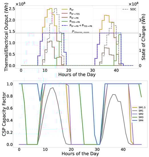
Figure 1.
Top: Time evolution of the thermal energies: Solar Field energy (PSF), Energy from Solar Field to Power Block (PSF→PB), Energy stored (PSF→TES), Energy discharged (PTES→PB) and Total available energy injected to the Power Block (Pin = PSF→PB +PTES→PB) and the State of charge (SOC) for a Solar Multiple (SM) of 1.5. Bottom: Capacity factors for SMs of 1, 2, 3 and 4.
Moreover, the bottom panel of Figure 1 allows us to compare, for the same two days as in the left panel, the resulting CFs for different SMs. One can see that, as the SM is increased, the mean of the CF increases, while its variance decreases, since the larger solar field allows us to store more energy to keep producing at nominal capacity the early evening (SM of 1.5 and 2) or later at night and the next day (SM of 3 and 4).
2.4. Optimization Experiments
To investigate the response of the Moroccan electricity mix to the integration of CSP with increasing storage capabilities, as measured by the SM, and examine the sensitivity of the optimal mix to rental cost (4) of PV and CSP, we carry out 6 optimization experiments summarized in Table 1.

Table 1.
Optimization experiments.
Thus, all combinations with CSP but PV-Wind-CSP-SM1 include storage. All combinations are optimized using the same value corresponding to the PV-Wind-CSP-SM1.5 combination (i.e., 3.96 G€/yr).
2.5. Residual Load Duration Curve Diagnostics
The risk is an aggregate measure of the variability of the RE production which does not take into account the specific timing of the fluctuations. However, the RE production tend to be more valuable if it occurs during a peak load than during a low load. That is why we introduce, after the optimization step, several additional diagnostics that reflect the impact of temporal renewable variability and illustrate the contribution of each renewable technology to the reduction of different load bands (i.e., peak, mid and base load).
To give a graphical representation of these properties, we show in Figure 2 the Load Duration Curve (LDC) and the Residual Load Duration Curve (RLDC)—see Appendix B—obtained from the analysis of Section 3. The LDC is plotted in black and the RLDC for a particular optimal PV-Wind-CSP1.5 mix in green. To show the contribution of each technology to the RLDC, we also represent the RLDC with PV only (brown), wind only (blue) and CSP only (orange).
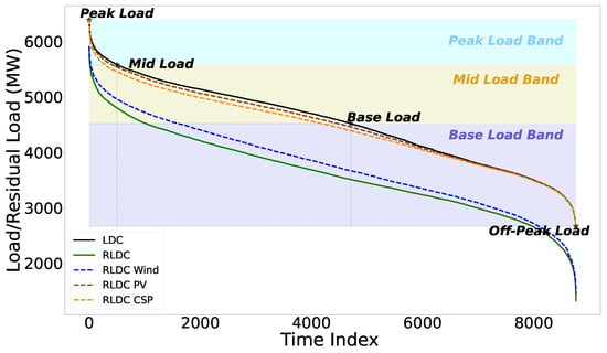
Figure 2.
LDC (plain black), RLDC (plain green), RLDC for PV only (dashed brown), RLDC for CSP only (dashed orange), and RLDC for wind only (dashed blue) for the optimal PV-Wind-CSP-SM1.5 mix for the global strategy with the maximum-cost constraint and at a mean penetration of 20%. See Section 3 for more information.
We divide the LDC and the RLDC into three intervals (vertical lines in Figure 2 delimiting the peak, mid and base time index). The peak load, associated with the 500 largest values; the mid load, associated with the 4706 largest values; and the base load, associated with all values between the peak and the off-peak load. The horizontal bands correspond to the load values of each load band. For each interval of the time index , we compute the load reduction by averaging the difference between the LDC and the RLDC over the band load time index and dividing the result by the total PV, wind and CSP capacity as following (10):
where and are the first and last time index of the load interval considered, is the peak load time index, is the residual peak load time index. For instance, here, we define the Capacity Credit (CC) as the peak-load reduction []. It is thus given by the for and . Similarly, the mid-load reduction (base-load reduction) is given by the for and (resp. and ). In addition, for each interval, the load reduction is decomposed into a contribution from each technology.
2.6. Data
2.6.1. Domain, Zones and Technologies
Morocco is located in the Maghreb region in North Africa. It is bordered to the North by the Strait of Gibraltar and the Mediterranean Sea, to the South by Mauritania, to the East by Algeria and to the West by the Atlantic Ocean (see the inset graph of Figure 3).
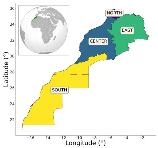
Figure 3.
Morocco’s electrical zones. Inset: Morocco’s undisputed territory (dark green) and Western Sahara (green), a territory claimed and occupied by Morocco.
To assign the administrative regions and the climatic grid cells to the electrical zones in E4CLIM, we use the geographical data downloaded from the Global Administrative Areas (GADM) online database (https://gadm.org/). The available data for Morocco do not include Western Sahara because it is considered a non-autonomous territory by the United Nations (UN)—as mentioned in the caption of Figure 3. Yet, the Moroccan electrical zones and the corresponding data provided by the ONE cover Western Sahara. We thus consider the region covered by Morocco and Western Sahara and concatenate the GADM data to define the electrical zones. The available administrative regions have been aggregated in the 4 electrical zones (Figure 3) referred as NORTH, CENTER, EAST and SOUTH.
Only wind, solar PV and CSP are considered as renewable energies in this study. Moreover, electricity power can flow unconstrained from any generation site to any demand site (no network constraints and no exchanges with other countries). Moreover, the mismatch between the demand and the renewable-energy production is not taken into account as the mean (1) and risk (2) from the optimization problem are used as proxies for the service needed from the conventional plants and imports.
2.6.2. Climate Data
We use input data over the year 2018 taken from the Modern Era Retrospective analysis for Research and Applications version 2 (MERRA-2) reanalysis []. The MERRA-2 reanalysis provides hourly values of surface pressure, temperature, density wind speed and downward radiation at the ground with a horizontal resolution of in latitude and longitude, respectively.
2.6.3. Demand Data
To fit the electricity demand model, the National Office of Electricity (ONE) provides us with a complete time series of hourly electricity demand for Morocco in 2018. For that purpose, a time series of the national demand is broken down by electrical zone using scaling factors provided by the ONE and based on the size, population density and economic activity of each zone. These factors are of 10%, 83%, 5% and 2% for the NORTH, CENTER, EAST and SOUTH zones, respectively. The national calendar of public holidays for Morocco, used to separate the impact of working days, Saturdays and days-off on the electricity demand is collected from the web portal (https://publicholidays.africa/). The yearly-means of the fitted demand are reported in Table 2.
Table 2.
Predicted yearly demand for 2018 (fitted) and CFs averaged over the same year (after bias correction) per zone and technology.
2.6.4. Capacity Factor Data and Bias Correction
Once the regional wind, PV and CSP CFs are computed at each grid cell of the MERRA-2 reanalysis, they are spatially averaged over each zone. Then, the CF prediction is statistically adjusted to 2018 observations so that the hourly CFs computed from the climate data are rescaled for their averages over the year 2018 to coincide with the averages of the observed CFs over the same year (Appendix C.2). For zones where no data are available for a given technology (marked by an empty set ∅ in the Table A2 and Table A3), a bias corrector averaged over all available zones for that technology is applied to the CF computed from the climate data for that zone and technology.
We compute the CFs, for each technology and zone, from the 2018 wind, PV and CSP installed capacities, for all k, and productions given in the Table A2 and Table A3, respectively. The geographical distribution of capacities presented in Table A2 is also represented in Figure A1. The data are derived from Table A4 where we compile data from various sources. For the CSP, only the Noor 2 and Noor 3 power plants in CENTER are selected to compute a CF corresponding to a SM of 1.5. The reference capacities are also used to compute the maximum total cost (5).
The yearly-means of the resulting corrected CFs and the predicted yearly demand for 2018 are reported in Table 2 for each zone and technology. It shows that wind CFs are the largest, with CSP CFs following before PV CFs. It thus appears that solar tracking by parabolic CSP more than compensates for the absence of conversion of diffuse radiation compared to PV.
It is important to note that, although higher SMs are obtained by increasing the SF area, the bias correction is bringing the means of the CFs for different SMs to a similar value. This is the effect looked after since the corresponding costs (see Section 2.6.5) are kept the same even though larger SF areas should in principle cost more. On the other hand, the variance of the CFs is decreased for higher SMs thanks to the relative increase in storage. Doing so, the optimization problem is only sensitive to the change of the variance associated with the change of the SM (see discussion of the maximum-penetration ratios and the minimum-variance ratios in the next Section 3).
2.6.5. Cost Data
Except for the discount rate, the economic data needed to compute the yearly rental cost (4) come from the scenario-based cost trajectories to 2050 of the European Commission Joint Research Center (JRC) [] for the year 2015. They include the following power production technologies: onshore wind turbines with medium specific capacity and medium hub height, utility-scale PV without tracking and parabolic trough with 6 to 8 hours storage (equivalent to SM1.5). In our study, we neglect the cost of TES capacity as TES is cheap []. The system cost is much more sensitive to the cost of the power technologies than to the cost of storage []. The cost of CSP is kept the same for different SMs, as discussed in the previous Section 2.6.4. A real discount rate has been evaluated between of 4 and 5% in Morocco ([], p. 27), so a value of 4.5% is used, in this study, for all technologies. This cost data and the resulted yearly rental cost—calculated using Equation (4)—are summarized in Table 3. It shows that the rental costs of wind and PV are relatively comparable, while they are more than four times lower than that of CSP.
Table 3.
Capital investment, fixed operation and maintenance costs, lifetime are from the European Commission Joint Research Center (JRC) technical report [] for the year 2015 (see Tables 12 and 10 for PV, Tables 2 and 5 for wind and Tables 15 and 16 for CSP), the discount rate is from the Design and Sustainability of Renewable Energy Incentives: An Economic Analysis Report ([], p. 27) and the yearly rental cost per technology calculated using Equation (4).
3. Results
Approximations of the fronts of the mean-variance problem (Section 2.1) are represented in the left panels of Figure 4 for the PV-Wind (top), PV-Wind-CSP SM1 (middle) and PV-Wind-CSP-SM1.5 (bottom) combinations. The corresponding plots are also represented in left panels of Figure 5 for PV-Wind-CSP-SM2 (top), PV-Wind- CSP-SM3 (middle) and PV-Wind-CSP-SM4 (bottom). The risk, , is in abscissa and the mean penetration (1), , in ordinate.
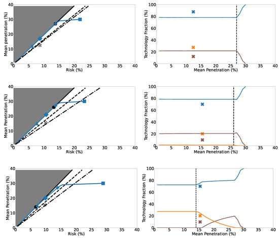
Figure 4.
Left: approximations of the fronts with the risk, σglobal/technology/base, in abscissa and the mean penetration (1), μ, in ordinate. Right: shares of wind (blue line), PV (brown line) and CSP (orange line) capacities versus the mean penetration for the global strategy with maximum-cost constraint. Top: PV-Wind. Middle: PV-Wind-CSP-SM1. Bottom: PV-Wind-CSP-SM1.5.
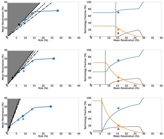
Figure 5.
Left: approximations of the fronts with the risk, σglobal/technology/base, in abscissa and the mean penetration (1), μ, in ordinate. Right: shares of wind (blue line), PV (brown line) and CSP (orange line) capacities versus the mean penetration for the global strategy with maximum-cost constraint. Top: PV-Wind-CSP-SM2. Middle: PV-Wind-CSP-SM3. Bottom: PV-Wind-CSP-SM4.
In each panel, different fronts are represented. Each point of the front represented by the plain blue curve is associated with a Pareto-optimal mix, taking into account correlations between technologies and zones (global strategy) while satisfying the maximum-cost constraint (3). The straight black line passing through the origin represents the front for the global strategy as well, but without the maximum-cost constraint. Points to the right of this front are not Pareto optimal. Points to the left of this front (in gray) are not feasible.
The 2018 mix, or actual mix, is represented by the gray cross. In addition, particular optimal mixes from the global front with the total-cost constraint are depicted. The blue triangle represents the optimal mix with the same penetration as the actual mix, namely the penetration-as-actual mix. The blue diamond represents the optimal mix with the same risk as the actual mix, namely the risk-as-actual mix. The blue square represents the optimal mix with the largest penetration, namely the maximum-penetration mix. The blue plus represents an optimal mix for which the maximum-constraint is activated but with moderate penetration, namely the cost-activated mix. The black dot is the point with the largest penetration to be on both the constrained (plain blue line) and unconstrained (plain black line) global fronts, namely the cost-activation mix. In other words, it represents the optimal mix with the highest penetration for which the maximum-cost constraint is not active.
The right panels of Figure 4 and Figure 5 represent, as a function of the penetration and for the constrained global front and different combinations, the shares of wind (blue line), PV (brown line) and CSP (orange line) capacities summed over all zones. The blue, brown and orange crosses represent respectively the shares of wind, PV and CSP capacities for the actual mix. The dashed vertical line is the penetration level to the right of which the maximum-cost constraint is active and corresponds to the black dot in the left panels.
In the following subsections, we examine common features for all combinations which help understand the general behavior of the model, draw insights on the sensitivity of the optimal mixes to the cost of solar technologies and the CSP’s SM, and evaluate the effect of TES and of correlations between Capacity Factors (CFs)—for different zones and/or technologies—on the risk adequacy.
3.1. Optimal Mixes Features Common to All Combinations
Comparing the panels from Figure 4 and Figure 5, some features of the fronts and technology shares remain unchanged from one combination to the other. The results are qualitatively different at low and at high penetrations.
3.1.1. At Low Penetrations
As long as the constrained global front (plain blue) coincides with the unconstrained one (straight black) at low penetrations, the shares of the different technologies in the mix are independent of the penetration (see the side of the right panels of Figure 4 and Figure 5 to the left of dashed line). At such low penetrations, little capacity is invested in so that the maximum-cost constraint is satisfied without activation. In fact, we show in Appendix D.3 that as long as the maximum-cost constraint is inactive and if we assume that all the cross-correlations between the normalized CFs are zero (i.e., if the covariance matrix is diagonal), all optimal capacities are positive and proportional to what we call the minimum-variance ratios and can be estimated by Equation (11):
In this case, the optimal mixes are not sensitive to rental costs. The minimum-variance ratios are given in Table 4. Different renewable combinations lead to differences in this ratio (see Section 3.2).
Table 4.
Minimum-variance ratios () given by (11).
To investigate the role played by correlations between CFs for different zones (regional diversification) and technologies (technological diversification), we compare the global (black line), technology (dashed black line) and base (point-dashed black line) fronts without the maximum-cost constraint (left panels of Figure 4 and Figure 5). These unconstrained fronts agree with the corresponding fronts with the maximum-cost constraint (only the global one being represented, in blue) only at low penetrations, when this constraint is inactive. They thus help understand the role of correlations at low penetrations only. In the technology strategy, all correlations between different zones are ignored, while, in the base strategy, correlations between different technologies of the same zone are also ignored (Section 2.1). These fronts are straight lines with a slope given by the mean-risk ratio (12),
at any point on the front. This ratio quantifies the increase in percentage point in the mean penetration achieved by letting the standard deviation rise by one point. Its values for the three strategies and six combinations are reported in Table 5.
Table 5.
Mean-risk ratios (12) of the global, technology and base fronts without the maximum-cost constraint for the different combinations.
We can see that the ratios decrease from the global to the base front so that the technology front is flatter than the global front and the base front flatter than the technology front. This shows that ignoring correlations between different zones and between different technologies of the same zone prevents reducing the risk as much as possible. The impact differs between combinations (see Section 3.2).
3.1.2. At High Penetrations
At high penetrations, the constrained front shows a larger risk than the unconstrained one, as the maximum-cost constraint prevents the investment in more capacity. As a result, technology shares are no longer constant at such high penetrations. As the penetration is increased, the wind share increases in all combination at the expense of the solar technologies.
As seen in Figure 4 and Figure 5, wind is dominating the point on the constrained front with the highest penetration (blue square in the left panels) which is the limit beyond which it is not possible to further increase the penetration while satisfying the maximum-cost constraint and the positivity bounds on capacities. At this point, wind penetration approaches 100%. As demonstrated in Appendix D.1 and taken numerical accuracy into account, this mix is such that only one capacity is positive, the one of the zone i and technology j, for which the quantity (13) that we call the maximum-penetration ratio,
is maximized. In fact, if the CFs were not normalized by the total demand, these ratios would be the inverse of the levelized cost of electricity for a given technology in a particular zone multiplied by the number of hours in a year.
If maximizes (13), then and for all . This ratio is thus maximized when the expectation of the CF over the total demand is large and when the rental cost is small. The maximum-penetration ratios for each technology and zone depend on the costs (Table 3) and average demand and CFs (Table 2), and are given in Table 6.
Table 6.
Maximum-penetration ratios (yr/T€) given by (13).
The maximum-penetration ratios are larger for wind than for PV, and larger for PV than for CSP. This helps to understand why, whatever the combination including CSP, CSP is first replaced by PV which is then replaced by wind as the penetration is increased and the maximum-cost constraint becomes more and more active. Eventually, only wind capacity in EAST remains whatever the combination. Thus, the maximum-penetration mix represented by the blue square in the left panels of Figure 4 and Figure 5 is located at the same point in the mean-risk plane for all combinations.
Optimal mixes for penetrations lower than the maximum tend to include a positive share of PV, whatever the combination. As shown in Appendix D.2, when the maximum-cost constraint is active and if is the index of the capacity which is installed to maximize the mean penetration, the first capacity that is installed after for lower penetrations is the one that minimizes the quantity (14),
In addition to identify the second capacity to be installed as the penetration is decreased from its maximum, it reveals the role of covariances between CFs of different technologies and zones. This quantity is minimized when the maximum-penetration ratio (13) of is large compared to that of already installed, when the correlation between and is small and when the standard deviation of normalized CF of divided by its cost is small (resp. large) compared to that of if the correlation is positive (resp. negative).
The ratios for each technology and zone are displayed in Table 7. We can see that, the ratio for wind in SOUTH is the smallest. We verify that this is indeed the second capacity to be installed by the numerical model when the penetration is decreased from its maximum (not shown here).
Table 7.
Ratios (no units) given by (14) to identify the second capacity to be installed as the mean penetration is decreased from its maximum.
Last, we can see that the actual mix (gray cross in the left panels of Figure 4 and Figure 5) is to the right of the constrained global front (blue line), whatever the combination. As a result, this mix has a larger risk than the penetration-as-actual mix (blue triangle) and a smaller penetration than the risk-as-actual mix (blue diamond). This shows that the current geographical and technological distribution of PV, wind and CSP in Morocco is sub-optimal and could be optimal (on the blue line) if the risk is reduced or the penetration is increased. For instance, according to the model, if all the CSP in Morocco had a SM of 1.5 (Figure 4f), the actual risk could be reduced by increasing the wind and CSP shares and removing PV completely. Increasing the share of CSP would also lower the risk for higher SMs (Figure 5).
3.2. Optimal Mix Differences between Combinations
The main interest of this study lies in the differences between combinations. We first observe, by comparing Figure 4b with Figure 4d, that the introduction of CSP without storage (SM1) does not significantly affect the optimal technology shares. Little CSP is indeed introduced at the expense of PV, but PV remains largely dominant over CSP. At high-penetrations, when the maximum-cost constraint is active, this can be understood from the fact that the larger CFs of CSP-SM1 (Table 2) are not able to compensate for the higher cost of CSP compared to PV (Table 3), as shown by the larger maximum-penetration ratios (Table 6) and as discussed in the previous Section 3.1.
At low penetrations, the lower share of CSP-SM1 compared to PV is explained by its lower minimum-variance ratios (Table 4). Indeed, the standard deviations of the CSP-SM1 and PV CFs being comparable (ignoring differences associated with diffuse radiation harvesting and solar tracking by CSP or efficiency response to temperature changes), the lower minimum-variance ratios of CSP-SM1 are due to the larger means of the CFs of CSP-SM1 compared to PV (Table 2) and to the fact that the CF variances tend to scale quadratically with the CF means, to first approximation. Assume for instance that the hourly CSP-SM1 CF is 1.5 that of the PV CF. Then the mean of the former is 1.5 that of the latter, but its variance is that of the latter, so that the minimum-variance ratio of this CSP-SM1 CF is 1.5 smaller than that of this PV CF.
However, with storage (Figure 4b and Figure 5b,d,f), CSP replaces PV completely. For combinations without CSP or for small SM (SM < 2), the large value of the minimum-variance ratio for wind in SOUTH (Table 4)—due to the high and regular CF of wind in this zone (Table 2)—explains its predominance at such low penetrations (Figure 4b–f and Figure 5b). However, the larger the SM—i.e., the larger the surplus of energy available for storage—the higher the share of CSP compared to wind, particularly for SM > 2 (Figure 5d,f).
The high share of CSP-TES compared to PV and wind at low penetrations can be understood from the fact that the CSP minimum-variance ratios increase with the SM to become larger than the ones for wind and PV (Table 4), because of the reduction of the variance of the CSP CFs with the increase of the amount of energy available for storage. The reduction of the CSP-CF’s variability due to storage thus results in a decline of the optimal-mix risk for a given low penetration. On the other hand, at penetrations beyond which the maximum-cost constraint is active, the share of CSP decreases for increasing SMs since installing more CSP at a higher cost than PV and wind also means reaching the maximum budget sooner. Thus, having more CSP at low penetrations does not imply that significantly more CSP is installed at higher penetrations unless the maximum total cost is increased.
The effect of correlations on the optimization also varies between combinations. For PV-Wind, the reduction of the mean-risk ratio (Table 5 and Figure 4a) is significant from the global to the technology strategy, but less so from the technology to the base strategy. This can be understood from the fact that correlations between different zones for the same technology are large (climatic conditions vary little within Morocco) and must be taken into account. On the other hand, correlations between irradiation and wind speed are weaker so that taking them into account is not as critical.
With the introduction of CSP without storage, however, the difference between the technology and the base fronts are much larger (Table 5 and Figure 4c). In this case, correlations between PV and CSP are large since the production of both is directly linked to temporal availability of the solar resource (even if CSP harvests the direct radiation only which is compensated by solar tracking). Ignoring these correlations thus leads to installing too much PV and CSP capacities, which results in an increased risk.
As the SM is increased (Figure 4e and Figure 5a,c,e), however, the difference between the technology and the base front weaken. The increased available storage indeed results in weaker correlations between PV and CSP. The differences between the global and the technology fronts are also reduced, due to the fact that the mixes become less diversified as CSP in SOUTH becomes dominant (Table 4).
3.3. Peak-, Mid- and Base-Load Reduction Diagnostics
For a more detailed description of the variability of the RE production, we now look at properties of specific mixes along the LDC/RLDC defined in Section 2.5.
Whatever the combination, we select optimal mixes on the constrained global frontier at three different levels of penetration: 16%, 20% and 27% which correspond to the penetration of the actual, risk as actual, and cost-activated mix of the PV-wind-CSP-SM1.5 combination, respectively. The maximum-cost constraint at 27% penetration is active for all combinations.
The properties of these mixes are presented in Table 8, Table 9 and Table 10, respectively. These properties are: the risk; the total PV, wind and CSP capacity; the shares of PV, wind and CSP capacity; the peak-load (CC), mid-load and base-load reductions; and the contribution from each technology.
Table 8.
Properties of the optimal mix at 16% penetration for the global strategy with the maximum-cost constraint and for different combinations.
Table 9.
Properties of the optimal mix at 20% penetration for the global strategy with the maximum-cost constraint and for different combinations.
Table 10.
Properties of the optimal mix at 27% penetration for the global strategy with the maximum-cost constraint and for different combinations.
We can see from the tables that the capacity credit (CC) decreases and reach a saturation value with increasing penetration whatever the combination. This saturation effect shows that additional PV, wind or CSP capacities are less efficient at providing peak load at higher penetrations. This does not mean that less conventional capacity can be replaced by RE in absolute terms, but rather that an additional RE plant tends to serve the peak load less per unit of capacity than previously installed RE plants do. This is also true for the mid-load reduction and the base-load reduction. Moreover, at the penetrations considered here, there is no curtailment. In other words, the RE production never exceeds the demand, so that the demand is never entirely satisfied by REs and no RE production is lost. Otherwise, CSP with TES could have played a role in limiting the amount of energy curtailed by flattening the production daily cycle.
The load reductions are mostly due to wind. The representation of the LDC and RLDCs for the optimal PV-Wind-CSP-SM1.5 combination for the global strategy with the maximum-cost constraint and a mean penetration of 20%, Figure 2, illustrates this effect. It is, however, associated with the high wind shares and does not necessarily mean that the solar technologies do not contribute to reduce the load efficiently in relative terms.
In addition, at penetrations including significant shares of CSP (Table 8 and Table 9) the CC tends to be higher for combinations with CSP with storage than for combinations without. Moreover, the decomposition of the CC by technology shows that the increase in the CC for combinations with storage is mostly due to CSP rather than to PV. Thus, in addition to reducing the risk, the introduction of CSP with storage helps satisfy peak loads more than PV or wind at equivalent shares. CSP with storage thus appears to be able to produce during hours of high loads (consistent with []). However, while further increasing the SM may help increase the CC, this also depends on the share of CSP in the mix, since the load reductions are based on CSP but also on PV and wind.
For wind, the base-load reduction is larger than the mid-load reduction, which is larger than the CC, for all three penetrations. Thus the larger the load, the less wind contributes to it, as is also visible in Figure 2. For PV and CSP without storage, the mid-load reduction is larger than the base-load reduction, which is larger than the CC, for all three penetrations. These technologies thus contribute mainly to the mid load and little to the peak load, as is also visible in Figure 2. That their contribution to the base load is weak can be understood from the fact that they do not generate at night when the load is small. On the other hand, for CSP with storage, the mid-load reduction is larger than the CC, which is larger than the base-load reduction. Thus, while the addition of storage does not change the fact that CSP mainly contributes to the mid load, it helps improve the CC significantly, in agreement with the previous paragraph.
4. Summary and Discussion
We study the response of regional Renewable Energy (RE) mix—including Solar Photovoltaic (PV) and wind energy as well—to the integration of Concentrated Solar Power (CSP) with Thermal Energy Storage (TES). We take as objective not only to maximize the production at a given cost, but also to provide adequacy services to the electricity system by reducing the variability of the RE production. To this end, we take the variance of the RE production—stemming from meteorological fluctuations—compared to the demand as proxy for the adequacy risk, thus resulting in a mean-variance analysis. This bi-objective optimization problem is implemented in the E4CLIM modeling platform [], which allows one to simulate hourly Capacity Factors (CFs) and demand profiles adjusted to observations from climate data. We adapt E4CLIM to Morocco and its four electrical zones for the year 2018, as a special case, add new CSP and TES simulation modules to it, and use additional diagnostics. To take the different rental costs of PV, wind and CSP into account, we take a recommissioning approach, in which the total rental cost of a mix is constrained to be lower than that of the actual 2018 Moroccan mix. We evaluate the impact of rental cost and CSP storage duration on the optimal mixes together with the role of technological and regional diversification. To do so, we analyze mixes along Pareto fronts—from low RE penetrations and low risks to high penetrations and high risks—including: PV and wind only; PV, wind and CSP without storage; and PV, wind and CSP with four increasing levels of storage (i.e., SM1), as measured by the Solar Multiple (SM1.5, 2, 3 and 4).
Due to the maximum-cost constraint we identify two regimes along the optimal fronts: one at low penetrations where only the mean vector and covariance matrix (variances and covariances) of the CFs (normalized by the total demand) play a role; and one at high penetrations where the rental cost of each technology also matters. At low penetrations, the share of each technology is constant. Wind dominates over PV and CSP without storage because the wind is stronger and more regular in the SOUTH zone on average. However, increasing the surplus of CSP available for TES—as measured by the SM—makes the CSP production more regular and favors the installation of CSP at low penetrations. This results in a decrease of the optimal-mix risk.
In addition, because variations in climatic conditions from one zone to the other are relatively small, it is essential to take correlations between CFs of different zones into account in order to reduce the risk as much as possible, whatever the technological combination. This is less true concerning correlations between the PV and wind CFs in the same or in different zones since these correlations are relatively small, different resources being harvested by these two technologies. It is, however, essential to take the strong correlations between the CSP-without-storage CFs and the PV CFs into account. As the SM is increased, however, the CSP profiles flatten. The role played by correlations between CSP CFs and CFs from other technologies is thus less important for such high SMs.
At high penetrations, the maximum recommissioning budget allowed becomes a limiting factor. Consequently, in addition to the variances and correlations, the cost of each technology compared to the CF mean (in our case, an analog of the Levelized Cost of Electricity, LCOE) contributes to determining which technology is installed in which zone in priority. Wind capacities are preferably installed, followed by PV—the rental costs of wind and PV being comparable and being much smaller than that of CSP and the mean wind CFs being higher than the mean PV CFs—so that technology shares are no longer constant relatively to the penetration.
The definition of the risk based on the variance of the RE production with respect to the demand that we use is not sensitive to the timing of RE fluctuations. By diagnosing the reduction of some measure of the peak, mid and base loads, we give a more detailed analysis of the service provided by each RE technology. We find that, while CSP contributes to reducing the mid load similarly to PV, adding TES to CSP significantly increases the overall RE capacity credit of the optimal mixes.
These results allow us to discuss the role of CSP-TES compared to PV and wind in reducing the adequacy risk by mitigating the variability of the RE production. They show that introducing CSP-TES, in particular with large SMs, reduces the risk. For instance, according to the model, we find that the risk of the actual 2018 Moroccan mix could be reduced by increasing the share of CSP-TES compared to PV. Yet, our model favors CSP with TES mostly at low penetrations due to the fixed total-cost constraint. However, if a high penetration is to be reached while preventing the risk to go past a given reliability threshold, more investment in RE is necessary. The smaller this threshold, the more likely is a high share of CSP-TES with a large SM to be optimal compared to PV. Thus, while the low LCOE of PV compared to CSP may motivate producers and planners to install more PV than CSP today when the RE penetration in Morocco not as large as what is aimed for, planning an efficient energy transition towards a high penetration may require steering the energy market to favor CSP-TES over PV, along with regional diversification.
Our definition of the risk is, however, based on the heuristic that the more variable the RE production, the more adequacy services will be required to satisfy the electricity demand at all times. This choice facilitates performing sensitivity analyses akin to the one conducted here, taking the RE-production variability into account while avoiding having to model the whole energy system. Yet this is at the cost of providing only an imperfect measure of the system cost. Our analysis thus allows us to stress the role of CSP-TES in providing adequacy services, but the current set up is too crude to make operational recommendations for the Moroccan energy transition, in particular regarding a quantitative estimate of the optimal shares of CSP-TES and PV, let alone the optimal distribution of SMs for CSP plants. For instance, the variance-based risk does not account for the superior ability of CSP with storage to meet peak demand—as measured by the capacity credit and observed in our analysis—compared to PV and wind.
A step in this direction while preserving the tractability of the optimization problem is to compare the response of the Moroccan mix to the integration of CSP with thermal storage to PV or wind deployed with battery or Pumped Hydro Storage (PHS); to imports/exports model or to demand-response mechanisms such as peak shaving or load-shifting. These flexibility modules could be simulated to evaluate their impact on the optimal mix in terms of cost and adequacy risk. The modeling framework could also be extended to monitor greenhouse-gas emissions associated with a given mix in order to directly take the reduction of these emissions as objective while controlling the system cost derived from a simplified microeconomic problem [].
Author Contributions
Conceptualization, A.-a.B., A.T., P.D.; Data curation, A.-a.B.; Formal analysis, A.-a.B., A.T., P.D.; Funding acquisition, A.-a.B.; Investigation, A.-a.B., A.T., P.D.; Methodology, A.-a.B., A.T., P.D.; Project administration, P.D., A.T., A.-a.B.; Software, A.T., A.-a.B.; Supervision, P.D., A.T.; Validation, P.D., A.T.; Writing—original draft, A.-a.B.; Writing—review & editing, A.T., A.-a.B., P.D.; Decision to publish the results, P.D., A.T., A.-a.B. All authors have read and agreed to the published version of the manuscript.
Funding
This research leading to these results has received funding from the Moroccan company MED-OCEAN through a Ph.D. scholarship.
Acknowledgments
This work was conducted in the frame of the Energy4Climate Interdisciplinary Center (E4C) of Institut Polytechnique de Paris and Ecole des Ponts ParisTech, supported by the MED-OCEAN research contract. The E4CLIM open-source software is supported by the 3rd Programme d’Investissements d’Avenir 345 [ANR-18-EUR-0006-02] and by the Foundation of Ecole polytechnique (Chaire “Défis Technologiques pour une Énergie Responsable”). The authors would like to acknowledge the National Electricity Office (ONE) in Morocco for providing the regional hourly load data. We are also grateful to the reviewers for taking the time to provide valuable comments and suggestions.
Conflicts of Interest
The authors declare no conflict of interest.
Data Availability
The data used in this study are available upon reasonable request to the authors. Some data used to support the findings of this study are included within the article.
Appendix A. Solar Field and Power Block Modeling
Appendix A.1. Main Characteristics of the 50 MW Reference CSP-TES Plant
We present in Table A1 the technical parameters of the 50 MW reference CSP-TES plant mentioned in Section 2.3.
Table A1.
Main characteristics of the 50 MW CSP-TES Andasol 1 power plant adapted from Silva et al. [] (Appendix A).
Table A1.
Main characteristics of the 50 MW CSP-TES Andasol 1 power plant adapted from Silva et al. [] (Appendix A).
| Property | Symbol | Value |
|---|---|---|
| Total aperture area | 510,120 m | |
| Row distance between collectors | m | |
| Collector length | 150 m | |
| Collector aperture width | m | |
| Focal length | f | m |
| SF inlet temperature | 293 | |
| SF outlet temperature | 393 | |
| CSP nominal power | 50 MW |
Appendix A.2. Solar Field Modeling
Here, we present the equations needed to compute the overall SF efficiency (Equation (7)).
The overall geometrical efficiency is given by Equation (A1):
where is the cos-loss efficiency, is the Incidence Angle Modifier-loss efficiency, S is the shading-loss efficiency, and R is the row-end-loss efficiency. The cos-loss occurs when the sun rays are not perpendicular to the aperture area of the collector. The angle is the incidence angle for a plane rotated about a horizontal east-west axis with continuous north-south tracking. The latter allows the collectors to operate longer during the day and the energy generated to be more uniform. It is relevant for locations like Morocco where the variation of the daily irradiation over the year is small []. The cos-loss is determined by Equation (A2):
where is the angle of incidence, the solar declination and the hour angle. When the sun is not perpendicular to the collector plane, it affects the rays reflection and hence the receiver absorption. The IAM is the variance in output performance of a solar collector as the angle of incidence changes in relation to the collector plane. The IAM factor is here given by Equation (A3) and laid its formulation from []:
The losses due to shading occurs at low solar altitude angles until a critical zenith angle is reached and depends on the distance between collector rows . The shading loss S is given by Equation (A4) [,],
where is the effective mirror width and the mirror width. The quantity S ranges between 0 (full shading) and 1 (no shading). Finally, if the sun beam upon a collectors’ edges is reflected but does not hit the receiver, a part of the receiver with the length does not contribute to the heat production. The row-end loss factor is thus written as follows (A5) [,],
where f is the focal length of the collector and is the collector length.
Optical losses are caused by imperfect reflection, transmission and absorption of the collectors []. The overall optical efficiency of the collectors, , is assumed constant and set to 73%.
Thermal losses occur on the receiver, connections and piping. Only the receiver losses are considered and are caused by the difference between the average fluid temperature , with and are the SF inlet and outlet temperatures, and the temperature of the receiver cover which is here 37 higher than the temperature of the surrounding ambient air obtained from the climate data (Section 2.6.2). Conduction losses are neglected. We write the radiation loss as follows (A6):
where the Stefan-Boltzmann constant, is the receiver area, C is the concentration ratio (i.e., ) set to 71, and the receiver emissivity (equal to 0.08 for absorbing pipes with ceramic-metal material) [].
The natural convection losses between the cover and the ambient air can be expressed by Equation (A7):
where the parameter is the loss coefficient of the receiver set to 2 W m K which is a low value because of the coating and the vacuum between the absorbing pipe and cover [].
The incident solar energy collected by the receiver is . The total thermal efficiency is therefore given by Equation (A8):
The forced convection (i.e., by strong winds) is neglected. Finally, the collectors’ availability is set to 99.5%.
Appendix A.3. Power Block Modeling
Here, we describe the parameters needed to compute PB efficiency (Equation (9)).
The quantity represents the parasitic loss, which corresponds to the electrical needs for the plant operation. It varies roughly between 4% and 13% of the nominal gross power output of the plant [], we set it to 4%.
The term is the constant thermodynamic efficiency of an ideal Clausius-Rankine cycle. Given the enthalpy , and corresponding to each state of the temperature-entropy diagram of the Rankine cycle for dry cooling [], it is here equal to 37.6%. Then, the thermal power of the turbine is calculated by Equation (A9):
where is defined in Section 2.3.3.
The generator efficiency, , is approximated by the following Equation (A10) [],
Appendix B. Residual Load Duration Curve Diagnostics
We explain, here, the details required to understand the diagnostics (Section 2.5) computed after the optimization is done. The Load Duration Curve (LDC), black line in Figure 2, measures the capacity-utilization requirements for each increment of load. A LDC is similar to a load time series but the demand data are ordered by decreasing values, rather than chronologically. There is thus a time index such that the demand D summed over all zones satisfies . The height of a LDC at a particular hour measures the required production at that hour. In this study, we analyze the hourly-sampled LDC for the year 2018 so that the number of samples is 8760.
The Residual Load Duration Curve (RLDC), green line in Figure 2, is similar to the LDC but the load is replaced by the residual load. The latter is defined as the total energy demand minus the total RE production, as stated in Equation (A12):
There is thus a time index such that the residual load satisfies for . RLDCs contain crucial information about the variability of wind and solar supply, as well as correlations with demand, thereby capturing major challenges of integrating renewable energies into power systems.
Appendix C. Data and Methods to Compute the Capacity Factors
Appendix C.1. Annual Observed Capacity Factors
The reference capacities and generation used to correct bias in the theoretical production models and to compute the capacity factors for each technology and zone (Section 2.6.4) are presented in Table A4 and summarized in Table A2, Figure A1 and Table A3.
Table A2.
Reference capacities per zone and technology installed in Morocco in 2018. Zone-technology pairs for which no capacity is installed are marked by an empty set ∅.
Table A2.
Reference capacities per zone and technology installed in Morocco in 2018. Zone-technology pairs for which no capacity is installed are marked by an empty set ∅.
| Zone | Capacity (MW) | ||
|---|---|---|---|
| Wind | PV | CSP | |
| NORTH | 396 | ∅ | ∅ |
| CENTER | 60.0 | 70.0 | 350 |
| EAST | ∅ | ∅ | ∅ |
| SOUTH | 759 | 100 | ∅ |
Table A3.
Yearly-mean generation averaged per zone and technology observed in Morocco in 2018. Zone-technology pairs for which no capacity is installed are marked by an empty set ∅.
Table A3.
Yearly-mean generation averaged per zone and technology observed in Morocco in 2018. Zone-technology pairs for which no capacity is installed are marked by an empty set ∅.
| Zone | Generation (TWh) | ||
|---|---|---|---|
| Wind | PV | CSP | |
| NORTH | 1.31 | ∅ | ∅ |
| CENTER | 0.210 | 0.12 | 1.21 |
| EAST | ∅ | ∅ | ∅ |
| SOUTH | 3.05 | 0.19 | ∅ |

Figure A1.
Observed PV, wind and CSP-TES capacity distribution per electrical zones in Morocco in 2018 corresponding to Table A2.
Table A4.
Characteristics of the wind, PV and CSP plants from Morocco operational in 2018. PT: Parabolic Trough CSP. ST: Solar Tower CSP. h: expected hours of storage. Based on [,], at the end of 2018, the total wind, PV and CSP capacities are MW, 170 MW and 530 MW, respectively. We ignore the production from auto-producers, except for wind plants since their installed capacity is included in the total wind capacity. Data from: MEME [], RES4MED [], Energypedia [], GEO [], CSP FOCUS [], SolarPACES [] and MASEN [].
| Power Plant Name | Techno. | Region | City | Cap. (MW) | Prod. (GWh/yr) | CF (%) | Year | Source |
|---|---|---|---|---|---|---|---|---|
| Abdelkhalek Torres/Koudia Al Baida | Wind | NORTH | Tetouan | 50 | 200 | 45.7 | 2000 | [] |
| Abdelkhalek Torres/Koudia Al Baida | Wind | NORTH | Tetouan | 3.5 | 12 | 39.1 | 2001 | [] |
| Lafarge | Wind | NORTH | Tetouan | 32 | 12 | 4.20 | 2005 | [] |
| Tangier1 (Dhar Saadane; Bni Jmel) | Wind | NORTH | Tanger | 140 | 510 | 41.6 | 2009 | [] |
| Haouma | Wind | NORTH | Ksar sghir | 50.6 | 200 | 45.1 | 2014 | [] |
| Jbel Sendouk/Khalladi | Wind | NORTH | Ksar sghir | 120 | 378 | 36.0 | 2018 | [] |
| Amougdoul | Wind | CENTER | Essaouira | 60 | 210 | 40.0 | 2007 | [,,] |
| CIMAR | Wind | SOUTH | Laayoune | 5 | 16 | 36.5 | 2011 | [] |
| Aftissat | Wind | SOUTH | Boujdour | 200 | 1000 | 57.1 | 2018 | [] |
| Akhfennir1 | Wind | SOUTH | Laayoune | 102 | 378 | 42.4 | 2014 | [] |
| Akhfennir2 | Wind | SOUTH | Laayoune | 102 | 378 | 42.4 | 2017 | [] |
| Foum El Oued | Wind | SOUTH | Laayoune | 50.6 | 200 | 45.1 | 2014 | [] |
| Tarfaya | Wind | SOUTH | Tarfaya | 300 | 1084 | 41.2 | 2014 | [] |
| Noor 4 | PV | CENTER | Ouarzazate | 70 | 120 | 19.6 | 2018 | [] |
| Noor Laayoune1 | PV | SOUTH | Laayoune | 80 | 150 | 21.4 | 2018 | [] |
| Noor Boujdour1 | PV | SOUTH | Boujdour | 20 | 40 | 22.8 | 2018 | [] |
| Noor 1 | CSP (PT, 3 h) | CENTER | Ouarzazate | 160 | 520 | 37.1 | 2016 | [,,] |
| Noor 2 | CSP (PT, 7 h) | CENTER | Ouarzazate | 200 | 699 | 39.9 | 2018 | [,,] |
| Noor 3 | CSP (ST, 7 h) | CENTER | Ouarzazate | 150 | 515 | 39.2 | 2018 | [,,] |
| Ain Beni Mathar | CSP (PT, 0 h) * | EAST | Jerrada | 20 | 55 | 31.4 | 2011 | [,] |
* The integrated solar combined-cycle power plan Ain Beni Mathar is composed of a 450 MW combined cycle and a 20 MW solar thermal system []. We consider only the solar part here.
==
Appendix C.2. Bias Correction Approach
The hourly bias corrected capacity factor is given by the following expression (A13):
where is the bias corrector, and correspond to hourly and yearly CFs. The brackets correspond to averages over all years available from the climate data.
Appendix D. Optimization Formulas
Here, we derive a few analytical results to help understand the behavior of the optimization program.
Appendix D.1. Maximum-Penetration Case
We first consider the case when the penetration is maximized. For that purpose, we leave out the variance term from the cost function. The Lagrangian corresponding to this single-objective maximization problem is given by the expression (A14):
where non-negative coefficient is the Karush-Kuhn-Tucker (KKT) multiplier associated with the maximum-cost constraint and is the vector of non-negative KKT multipliers associated with the positive-capacities constraint.
Due to the first-order condition and dual feasibility, the case with equal to 0 is impossible since this would imply the contradiction . Thus, is positive (i.e., the maximum-cost constraint is activated) and such that (A18),
and .
Let us define the index , such that . Then the capacities are ranked by decreasing maximum-penetration ratio, i.e., .
If , then for all , all capacities are 0, the maximum-cost constraint is not active and so , leading to a contradiction. Thus, and .
Finally, if , then one would exactly have (A19),
which, loosely, has a zero probability.
In conclusion, for all practical purposes, the mean penetration is maximized by installing all the capacity allowed by the maximum-cost constraint in the zone and technology with the highest maximum-penetration ratio (13), i.e., and .
Appendix D.2. High-Penetration Case
We now start from the situation maximizing the mean penetration, as described in the previous Section D.1 and start to give some weight to the variance. To proceed, we scalarize the bi-objective problem by introducing a positive weight q. The Lagrangian of the scalarized maximization problem is given by (A20):
The first-order condition becomes (A21),
and the slackness conditions are the same as in Section D.1.
The solution to this problem for is that of the previous Section D.1. Increasing q from this situation, we thus assume that is positive, so that is 0. If all other capacities remain 0, and the covariance between and k is small, the total-capacity constraint remains active () as long as (D.2),
We now increase q from 0, while remaining in the interval , so that , and look for the largest value of q such that all capacities but that of remain 0. In this case, is still equal to . In other words, we impose that for all different from . The first-order condition (A21) then implies (A22),
which is equivalent to, with , with (A23):
Thus, the first capacity to be installed after is the one for which the right-hand side of this last expression is the smallest.
Appendix D.3. Low-Variance Case
We now turn to the case for which the variance is small. The extreme case of zero variance corresponds to the situation where all capacities are 0 because no weight is put on the mean penetration.
Let us consider the less trivial situation in which a weight is put on the mean penetration. That is, we scalarize the mean-variance problem to yield a corresponding Lagrangian given by (A24),
The first-order condition becomes (A25),
Since , there is an interval , with , such that as long as r stays within this interval, the maximum-cost constraint is inactive, i.e., and .
Let us consider that r is increased from 0 while remaining in . If some cross-covariances are non-zero, it may be that some capacities are zero. If instead we assume that the covariance matrix is diagonal, i.e., that for all such that . The first-order condition (A25) implies (A26),
Thus, in this case, implies that .
As a conclusion, if the covariance matrix is diagonal and for r in , either and all capacities are 0, or and all capacities are positive and such that (A27),
References
- Trappey, A.; Trappey, C.; Tan, H.; Liu, P.H.Y.; Li, S.J.; Lin, L.C. The determinants of photovoltaic system costs: An evaluation using a hierarchical learning curve model. J. Clean. Prod. 2016, 112, 1709–1716. [Google Scholar] [CrossRef]
- IEA-PVPS. Snapshot of Global PV Markets. IEA, 2020. Available online: https://iea-pvps.org/wp-content/uploads/2020/04/IEA_PVPS_Snapshot_2020.pdf (accessed on 28 September 2020).
- DLR. Concentrating Solar Power for the Mediterranean Region. Report, 2005. Available online: https://www.dlr.de/tt/Portaldata/41/Resources/dokumente/institut/system/publications/MED-CSP_complete_study-small.pdf (accessed on 28 September 2020).
- DLR. Trans-Mediterranean Interconnection for Concentrating Solar Power. 2006. Available online: https://www.dlr.de/tt/Portaldata/41/Resources/dokumente/institut/system/projects/WP00_TRANS-CSP-Introduction_and_Summary-Final.pdf (accessed on 28 September 2020).
- Ramin Jalilvand, D. Renewable Energy for the Middle East and North Africa: Policies for a Successful Transition; Friedrich Ebert Stiftung: Berlin, Germany, 2012; Available online: http://library.fes.de/pdf-files/iez/08959.pdf (accessed on 28 September 2020).
- Azouzoute, A.; Merrouni, A.A.; Touili, S. Overview of the integration of CSP as an alternative energy source in the MENA region. Energy Strategy Rev. 2020, 29, 100493. [Google Scholar] [CrossRef]
- Richts, C. The Moroccan Solar Plan: A Comparative Analysis of CSP and PV Utilization Until 2020. Master’s Thesis, University of Kassel, Kassel, Germany, 2012. Available online: http://www.uni-kassel.de/eecs/fileadmin/datas/fb16/remena/theses/batch2/MasterThesis_Christoph_Richts.pdf (accessed on 28 September 2020).
- IRENA. Renewable Power Generation Costs in 2017; Report; IRENA: Abu Dhabi, UAE, 2018; Available online: https://www.irena.org/-/media/Files/IRENA/Agency/Publication/2018/Jan/IRENA_2017_Power_Costs_2018.pdf (accessed on 28 September 2020).
- IRENA. Renewable Power Generation Costs in 2019; Report; IRENA: Abu Dhabi, UAE, 2019; Available online: https://www.irena.org/-/media/Files/IRENA/Agency/Publication/2020/Jun/IRENA_Power_Generation_Costs_2019.pdf (accessed on 28 September 2020).
- Ondraczek, J.; Komendantova, N.; Patt, A. WACC the Dog: The Effect of Financing Costs on the Levelized Cost of Solar PV Power. Renew. Energy 2015, 75, 888–898. [Google Scholar] [CrossRef]
- Platzer, W.J. Combined Solar Thermal and Photovoltaic Power Plants: An Approach to 24 h Solar Electricity? In Proceedings of the SOLARPACES 2015 International Conference on Concentrating Solar Power and Chemical Energy Systems, Freiburg, Germany, 31 May 2016. [Google Scholar] [CrossRef]
- Schinko, T.; Bohm, S.; Komendantova, N.; Jamea, E.M.; Blohm, M. Morocco’s sustainable energy transition and the role of financing costs: A participatory electricity system modeling approach. Energy Sustain. Soc. 2019, 9. [Google Scholar] [CrossRef]
- Schinko, T.; Komendantova, N. De-risking investment into concentrated solar power in North Africa: Impacts on the costs of electricity generation. Renew. Energy 2016, 92, 262–272. [Google Scholar] [CrossRef]
- Hamilton, W.T.; Husted, M.; Newman, A.; Braun, R.; Wagner, M. Dispatch optimization of concentrating solar power with utility-scale photovoltaics. Optim. Eng. 2020, 21, 335–369. [Google Scholar] [CrossRef]
- REN21. Renewables 2018 Global Status Report; REN21: Paris, France, 2018; Available online: https://www.ren21.net/wp-content/uploads/2019/05/GSR2018_Full-Report_English.pdf (accessed on 28 September 2020).
- Albadi, M.H. Solar pv Power Intermittency and its Impacts on Power Systems? An Overview. J. Eng. Res. 2019, 16, 142–150. [Google Scholar] [CrossRef]
- Heide, D.; Bremen, L.V.; Greiner, M.; Hoffmann, C.; Speckmann, M.; Bofinger, S. Seasonal optimal mix of wind and solar power in a future, highly renewable Europe. Renew. Energy 2010, 35, 2483–2489. [Google Scholar] [CrossRef]
- Denholm, P.; O’Connell, M.; Brinkman, G.; Jorgenson, J. Overgeneration from Solar Energy in California: A Field Guide to the Duck Chart; Report; National Renewable Energy Laboratory: Golden, CO, USA, 2015. Available online: https://www.nrel.gov/docs/fy16osti/65023.pdf (accessed on 28 September 2020).
- Hirth, L.; Ueckerdt, F.; Edenhofer, O. Integration costs revisited—An economic framework of wind and solar variability. Renew. Energy 2014, 74, 925–939. [Google Scholar] [CrossRef]
- Sijm, J. Cost and Revenue Related Impacts of Integrating Electricity from Variable Renewable Energy into the Power System—A Review of Recent Literature; (ECN–E-14-022); Energie Centrum Nederland: Petten, The Netherlands, 2014. [Google Scholar]
- Bousselamti, L.; Cherkaoui, M. Modelling and Assessing the Performance of Hybrid PV-CSP Plants in Morocco: A Parametric Study. Int. J. Photoenergy 2019, 2019, 1–15. [Google Scholar] [CrossRef]
- Brand, B.; Stambouli, A.B.; Zejli, D. The value of dispatchability of CSP plants in the electricity systems of Morocco and Algeria. Energy Policy 2012, 47, 321–331. [Google Scholar] [CrossRef]
- Denholm, P.; Mehos, M. Enabling Greater Penetration of Solar Power via the Use of CSP with Thermal Energy Storage. Conc. Sol. Power Data Dir. Emerg. Sol. Technol. 2011. [Google Scholar] [CrossRef]
- Forrester, J. The Value of CSP with Thermal Energy Storage in Providing Grid Stability. Energy Procedia 2014, 49, 1632–1641. [Google Scholar] [CrossRef]
- Oukili, M.; Zouggar, S.; Seddik, M.; Vallée, F.; Hafyani, M.E.; Ouchbel, T. Evaluation of the Moroccan Power Grid Adequacy with Introduction of Concentrating Solar Power (CSP) Using Solar Tower and Parabolic Trough Mirrors Technology. Energy Procedia 2013, 42, 113–122. [Google Scholar] [CrossRef][Green Version]
- Oukili, M.; Zouggar, S.; Seddik, M.; Ouchbel, T.; Vallée, F.; Hafiani, M.E. Comparative Study of the Moroccan Power Grid Reliability in Presence of Photovoltaic and Wind Generation. Smart Grid Renew. Energy 2013, 4, 366–377. [Google Scholar] [CrossRef][Green Version]
- Denholm, P.; Jorgenson, J.; Miller, M.; Zhou, E.; Wang, C. Methods for Analyzing the Economic Value of Concentrating Solar Power with Thermal Energy Storage; Technical Report; National Renewable Energy Laboratory: Golden, CO, USA, 2015. Available online: https://www.nrel.gov/docs/fy15osti/64256.pdf (accessed on 28 September 2020).
- Alliance, C. The Economic and Reliability Benefits of CSP with Thermal Energy Storage: Literature Review and Research Needs; Report; CSP Alliance: United States, 2014; Available online: http://www.inship.eu/docs/TES%204%20the_economic_and_reliability_benefits_of_csp_with_thermal_storage_2014_09_09_final.pdf (accessed on 28 September 2020).
- Shirizadeh, B.; Perrier, Q.; Quirion, P. How Sensitive Are Optimal Fully Renewable Power Systems to Technology Cost Uncertainty? FAERE Policy Paper; CIRED: Paris, France, 2019; Available online: http://faere.fr/pub/PolicyPapers/Shirizadeh_Perrier_Quirion_FAERE_PP2019_04.pdf (accessed on 28 September 2020).
- Brown, T.; Bischof-Niemz, T.; Blok, K.; Breyer, C.; Lund, H.; Mathiesen, B. Response to ‘Burden of proof’: A comprehensive review of the feasibility of 100% renewable-electricity systems. Renew. Sustain. Energy Rev. 2017, 92, 834–847. [Google Scholar] [CrossRef]
- Schellekens, G.; Battaglini, A.; Lilliestam, J.; McDonnell, J.; Patt, A. 100% Renewable Electricity—A Roadmap to 2050 for Europe and North Africa. Report, 2010. Available online: https://www.pwc.co.uk/assets/pdf/100-percent-renewable-electricity.pdf (accessed on 28 September 2020).
- de Castro, C.; Capellán-Pérez, I. Concentrated Solar Power: Actual Performance and Foreseeable Future in High Penetration Scenarios of Renewable Energies. BioPhys. Econ. Resour. Qual. 2018, 3, 1–20. [Google Scholar] [CrossRef]
- Du, E.; Zhang, N.; Hodge, B.M.; Wang, Q.; Kang, C.; Kroposki, B.; Xia, Q. The Role of Concentrating Solar Power Towards High Renewable Energy Penetrated Power Systems. IEEE Trans. Power Syst. 2018. [Google Scholar] [CrossRef]
- Madaeni, S.H.; Sioshansi, R.; Denholm, P. How Thermal Energy Storage Enhances the Economic Viability of Concentrating Solar Power. Proc. IEEE 2012, 100, 335–347. [Google Scholar] [CrossRef]
- Guédez, R.; Spelling, J.; Laumert, B.; Fransson, T. Optimization of Thermal Energy Storage Integration Strategies for Peak Power Production by Concentrating Solar Power Plants. Energy Procedia 2014, 49, 1642–1651. [Google Scholar] [CrossRef]
- Guédez, R.; Topel, M.; Spelling, J.; Laumert, B. Enhancing the profitability of solar tower power plants through thermoeconomic analysis based on multi-objective optimization. Energy Procedia 2015, 69, 1277–1286. [Google Scholar] [CrossRef]
- Tizgui, I.; Guezar, F.; Bouzahir, H.; Vargas, A.N. Estimation and Analysis of Wind Electricity Production Cost in Morocco. Int. J. Energy Econ. Policy 2018, 8, 58–66. [Google Scholar]
- Mohamed, A.; Aboubakr, E.; Moussaoui, H.; El Markhi, H. Renewable Energy Potential and Available Capacity for Wind and Solar Power in Morocco Towards 2030. J. Eng. Sci. Technol. Rev. 2018, 11, 189–198. [Google Scholar] [CrossRef]
- Kost, C.; Pfluger, B.; Eichhammer, W.; Ragwitz, M. Fruitful symbiosis: Why an export bundled with wind energy is the most feasible option for North African concentrated solar power. Energy Policy 2011, 39, 7136–7145. [Google Scholar] [CrossRef]
- Petrollese, M.; Cocco, D. Optimal design of a hybrid CSP-PV plant for achieving the full dispatchability of solar energy power plants. Sol. Energy 2016, 137, 477–489. [Google Scholar] [CrossRef]
- Starke, A.; Cardemil, J.; Escobar, R.; Colle, S. Assessing the performance of hybrid CSP + PV plants in northern Chile. Sol. Energy 2016, 138. [Google Scholar] [CrossRef]
- Du, E.; Zhang, N.; Hodge, B.M.; Wang, Q.; Lu, Z.; Kang, C.; Kroposki, B.; Xia, Q. Operation of a High Renewable Penetrated Power System with CSP Plants: A Look-Ahead Stochastic Unit Commitment Model. IEEE Trans. Power Syst. 2018. [Google Scholar] [CrossRef]
- Rye, E.A.; Lie, A.; Svendsen, H.G. Analyzing large-scale renewable energy integration and energy storage in Morocco using a flow-based market model. In Proceedings of the 2016 13th International Conference on the European Energy Market (EEM), Porto, Portugal, 6–9 June 2016; pp. 1–5. [Google Scholar] [CrossRef]
- Alhamwi, A.; Kleinhans, D.; Weitemeyer, S.; Vogt, T. Optimal mix of renewable power generation in the MENA region as a basis for an efficient electricity supply to europe. EPJ Web Conf. 2014, 79, 03004. [Google Scholar] [CrossRef]
- Alhamwi, A.; Kleinhans, D.; Weitemeyer, S.; Vogt, T. Moroccan National Energy Strategy reviewed from a meteorological perspective. Energy Strategy Rev. 2015, 6, 39–47. [Google Scholar] [CrossRef]
- Alhamwi, A. Optimal mix analyses of renewable power generation in the MENA region: A case study for Morocco. Master’s Thesis, KASSEL University, Kassel, Germany, CAIRO University GIZA, Cairo, Egypt, 2013. Available online: https://www.uni-kassel.de/eecs/fileadmin/datas/fb16/remena/theses/batch3/MasterThesis_Alaa_Alhamwi.pdf (accessed on 28 September 2020).
- Tantet, A.; Stéfanon, M.; Drobinski, P.; Badosa, J.; Concettini, S.; Créti, A.; D’Ambrosio, C.; Thomopulos, D.; Tankov, P. e4clim 1.0: The Energy for a Climate Integrated Model: Description and Application to Italy. Energies 2019, 12, 4299. [Google Scholar] [CrossRef]
- Chentouf, M.; Allouch, M. Renewable and Alternative Energy Deployment in Morocco and Recent Developments in the National Electricity Sector. J. Photoenergy 2018, 2. [Google Scholar] [CrossRef]
- Merrouni, A.; Elalaoui, F.; Ghennioui, A.; Mezrhab, A. A GIS-AHP combination for the sites assessment of large-scale CSP plants with dry and wet cooling systems. Case study: Eastern Morocco. Sol. Energy 2018, 166, 2–12. [Google Scholar] [CrossRef]
- Ministère de l’Energie, des Mines et de l’Environnement (MEME). Available online: https://www.mem.gov.ma/pages/index.aspx (accessed on 28 September 2020).
- Justus, C.; Mikhail, A. Height variation of wind speed and wind distribution statistics. Geophys. Res. Lett. 1976, 3, 261–264. [Google Scholar] [CrossRef]
- Ioannis, T.; Dalius, T.; Andreas, Z. Cost Development of Low Carbon Energy Technologies—Scenario-Based Cost Trajectories to 2050; 2017 Edition (EUR 29034 EN); Publications Office of the European Union: Luxembourg, 2018. [Google Scholar] [CrossRef]
- Duffie, J.A.; Beckman, W.A. Solar Engineering of Thermal Processes, 4th ed.; WILEY: New York City, NY, USA, 2013; 944p. [Google Scholar]
- Markowitz, H. Portfolio Selection. J. Financ. 1952, 7, 77–91. [Google Scholar] [CrossRef]
- IRENA. Renewable Energy Technologies: Cost Analysis Series—Concentrating Solar Power; Report; IRENA: Abu Dhabi, UAE, 2012; Available online: https://www.irena.org/documentdownloads/publications/re_technologies_cost_analysis-csp.pdf (accessed on 28 September 2020).
- Khatib, N. Country Profile Morocco Report. RES4MED&Africa. 2018. Available online: https://www.res4africa.org/wp-content/uploads/2018/06/Country-profile-Marocco-2.pdf (accessed on 28 September 2020).
- Hale, E.; Stoll, B.; Mai, T. Capturing the Impact of Storage and Other Flexible Technologies on Electric System Planning; Report; National Renewable Energy Laboratory: Golden, CO, USA, 2016. Available online: https://www.nrel.gov/docs/fy16osti/65726.pdf (accessed on 28 September 2020).
- Gelaro, R.; McCarty, W.; Suárez, M.; Todling, R.; Molod, A.; Takacs, L.; Randles, C.; Darmenov, A.; Bosilovich, M.; Reichle, R.; et al. The Modern-Era Retrospective Analysis for Research and Applications, Version 2 (MERRA-2). J. Clim. 2017, 30. [Google Scholar] [CrossRef] [PubMed]
- Meier, P.; Vagliasindi, M.; Imran, M. The Design and Sustainability of Renewable Energy Incentive: An Economic Analysis Report; World Bank: Washington, DC, USA, 2015; Available online: http://hdl.handle.net/10986/20524 (accessed on 28 September 2020).
- Yong, P.; Cheng, L.; Zhu, H.; Tang, L.; Zhang, N.; Kang, C. Investigating the influence of storage on Renewable Energy Capacity Credit. In Proceedings of the 2019 IEEE Power Energy Society General Meeting (PESGM), Atlanta, GA, USA, 4–8 August 2019; pp. 1–5. [Google Scholar] [CrossRef]
- Cretì, A.; Fontini, F. Economics of Electricity: Markets, Competition and Rules; Cambridge University Press: Cambridge, UK, 2019; p. 214. [Google Scholar] [CrossRef]
- Silva, J.; Castro, R. Modeling and Simulation of a Parabolic Trough Power Plant. Green 2012, 2, 97–104. [Google Scholar] [CrossRef]
- Patnode, A. Simulation and Performance Evaluation of Parabolic Trough Solar Power Plants. Ph.D. Thesis, University of Wisconsin-Madison, Madison, WI, USA, 2006. Available online: http://digital.library.wisc.edu/1793/7590 (accessed on 28 September 2020).
- Moroccan Agency for Sustainable Energy (MASEN). Available online: http://www.masen.ma/fr/projets (accessed on 28 September 2020).
- MEDIA24 | Environnement. Energies Renouvelables: 3.685 MW de Puissance Installée à fin 2019. Available online: https://www.medias24.com/energies-renouvelables-3-685-mw-de-puissance-installee-a-fin-2019-6619.html (accessed on 28 September 2020).
- Energypedia. Available online: https://energypedia.info/wiki/Wind_Energy_Country_Analyses_Morocco (accessed on 28 September 2020).
- Global Energy Observatory (GEO). Available online: http://globalenergyobservatory.org/ (accessed on 28 September 2020).
- CSP Focus. Available online: http://www.cspfocus.cn/en/ (accessed on 28 September 2020).
- Solar Power and Chemical Energy Systems (SolarPACES). Available online: https://solarpaces.nrel.gov/ (accessed on 28 September 2020).
- Middle East and North Africa Concentrating Solar Power Knowledge and Innovation Program (MENA CSP KIP). Available online: http://cmimarseille.org/menacspkip/wp-content/uploads/2017/08/Youssef_Stitou_MENA_CSP_KIP_Jordan_Workshop_25_July_2017.pdf (accessed on 28 September 2020).
- Ain Beni Mathar: Une Centrale Électrique Thermo Solaire Unique au Maroc. Available online: https://www.afdb.org/fr/projects-and-operations/selected-projects/ain-beni-mathar-a-unique-thermo-solar-powerplant-in-morocco-142 (accessed on 28 September 2020).
© 2020 by the authors. Licensee MDPI, Basel, Switzerland. This article is an open access article distributed under the terms and conditions of the Creative Commons Attribution (CC BY) license (http://creativecommons.org/licenses/by/4.0/).