Article

Measuring the Risk of Supply and Demand Imbalance at the Monthly to Seasonal Scale in France

1
LMD-IPSL, Ecole Polytechnique, Institut Polytechnique de Paris, ENS, PSL Research University, Sorbonne Université, CNRS, 91120 Palaiseau, France
2
Laboratoire de Probabilités et Modèles Aléatoires, Université Paris Diderot-Paris 7, 75013 Paris, France
3
CREST, ENSAE Paris, Ecole Polytechnique, Institut Polytechnique de Paris, CNRS, 91120 Palaiseau, France
*
Author to whom correspondence should be addressed.
Energies 2020, 13(18), 4888; https://doi.org/10.3390/en13184888
Submission received: 6 August 2020 / Revised: 6 September 2020 / Accepted: 11 September 2020 / Published: 18 September 2020
(This article belongs to the Special Issue Systemic Issues to Wind and Solar Energy Deployment)

Abstract

:
Transmission system operator (TSOs) need to project the system state at the seasonal scale to evaluate the risk of supply-demand imbalance for the season to come. Seasonal planning of the electricity system is currently mainly adressed using climatological approach to handle variability of consumption and production. Our study addresses the need for quantitative measures of the risk of supply-demand imbalance, exploring the use of sub-seasonal to seasonal forecasts which have hitherto not been exploited for this purpose. In this study, the risk of supply-demand imbalance is defined using exclusively the wind energy production and the consumption peak at 7 pm. To forecast the risks of supply-demand imbalance at monthly to seasonal time horizons, a statistical model is developed to reconstruct the joint probability of consumption and production. It is based on a the conditional probability of production and consumption with respect to indexes obtained from a linear regression of principal components of large-scale atmospheric predictors. By integrating the joint probability of consumption and production over different areas, we define two kind of risk measures: one quantifies the probablity of deviating from the climatological means, while the other, which is the value at risk at 95% confidence level ( V a R 95 ) of the difference between consumption and production, quantifies extreme risks of imbalance. In the first case, the reconstructed risk accurately reproduces the actual risk with over 0.80 correlation in time, and a hit rate around 70–80%. In the second case, we find a mean absolute error (MAE) between the reconstructed and real extreme risk of 2.5 to 2.8 GW, a coefficient of variation of the root mean square error (CV-RMSE) of 3.8% to 4.2% of the mean actual V a R 95 and a correlation of 0.69 and 0.66 for winter and fall, respectively. By applying our model to ensemble forecasts performed with a numerical weather prediction model, we show that forecasted risk measures up to 1 month horizon can outperform the climatology often used as the reference forecast (time correlation with actual risk ranging between 0.54 and 0.82). At seasonal time horizon (3 months), our forecasts seem to tend to the climatology.

1. Introduction

Transmission System Operator (TSOs) have to ensure at all times the balance between supply and demand of electricity. Supply and demand balance is handled by complex relations between many actors of the energy market and electricity grid system, e.g., producers of electricity, traders, distributors, industrial consumers, etc. The management of the balance requires in advance planning of the electricity system which results in some flexibility allowing to face and react rapidly to potential imbalance between supply and demand. Ensuring this balance is a challenge issued at many timescales going from the second to several months.
In this paper, we address the issue of seasonal planning of the electricity system in France, in fall and winter seasons. Cold seasons display the highest risk in France because cold temperatures cause sharp increase of the consumption. The risk is also the highest at 7 pm during the daily peak of consumption, on which this study focuses. In France, the electricity production is dominated by nuclear power plants (>70% of the total production). Still, with the increasing share of variable renewable energy sources (mainly wind and solar energy sources), TSOs need to manage increasing variable production. In this study, we focus on wind energy production only mainly because wind energy contributes to cover the evening consumption peak contrary to solar energy production which is too small at the peak hours. It is also motivated by the strong penetration of wind energy sources in the French (and European) electricity grid system. However, the reader needs to keep in mind that, in reality, the seasonal risk is also impacted by the nuclear power plant availability and the level of the hydroreservoirs, as well as the exchanges of electricity through the European grid. Moreover, solar energy may also contribute to supply-demand balance at other time of the day. These issues are nevertheless out of the scope of this study.
In 2017, France ended with a total installed wind capacity of 13.5 GW. On 30 December 2017, the network integrated 11 GW from wind power plants. Other records were set in the summer 2017 with half-hourly consumption coverage rates approaching 25% [1]. Some scenarios of energy mix by 2030 predict 30% to 40% of consumption met by wind energy production in Europe [2,3], so that risk hazard due to intermittency is expected to increase. For instance, a cold winter characterized by weaker winds than normal may in some cases lead to a lack of energy if not enough other production means have been made available upstream to meet the energy demands. Accurate seasonal forecasting of wind production would allow TSOs to take into account the interannual wind variability in the seasonal risk assessment of supply and demand balance. Currently, the seasonal risk is addressed by comparing climatological scenarios of consumption with available production capacity given by producers. Renewable intermittent production is also usually assessed using climatological scenarios [4,5]. For instance, in [4] winter outlook report 2016, a study based on 14 climatic years shows risks of national electric production deficit, not always compensated by import from EU countries, in situations of high demand due to low temperatures (see Figure 17 in [4]). Though the demand met by wind energy production is still quite low in France (around 4.5 % ) and in Europe (around 12 % ), the variability of the wind energy production already impacts the seasonal risk of imbalance between supply and demand.
At the seasonal scale, the predictability of the weather is still an open question, especially at midlatitude. Some studies nevertheless highlight skillful forecasts of Numerical Weather Prediction models (NWP). Particularly, skill of ensemble forecast systems in predicting the North Atlantic Oscillation (NAO), which is a typical atmospheric pattern controlling the weather variability over Europe, has been demonstrated by [6]. They show that depending on the forecast ensemble size the correlation between observed and forecasted NAO seasonal index can be as much as 0.6 and theoretically may reach almost 0.8 . Reference [7] also shows that wind speed and solar irradiance are related with the NAO, as well as the arctic oscillation (AO) for instance, pointing out the potential predictability of wind speed and solar irradiance through such patterns. Reference [8] highlights such relation between NAO and the surface wind speed over a smaller domain covering Europe.
In the energy sector, studies on seasonal forecasts mainly focus on the assessment of NWP seasonal forecast ensemble to predict climate related variables such as temperature, wind speed and solar irradiance. For instance, the study of [9] gives a method for calibration of surface wind speed globally and analyse the gain of such method compared to simple bias correction in several areas. Reference [10] assesses the surface wind speed output from the seasonal forecast ensemble of European center and show predictability up to some weeks in the North Sea region. In the study of [11], the fact that surface wind speed is related to large-scale patterns such as NAO is used to predict surface wind speed up to 3 months. Reference [12] demonstrates skills of several seasonal forecasting models to predict the seasonal mean wind speed in Europe. Reference [13] goes further by computing the capacity factor before assessing the seasonal forecasts skill. They show that using their method, the forecast skill of the computed capacity factor is better than the those of the surface wind speed itself. Several studies investigate the co-variability of energy related variables. Among them, the study of [14] analyse the joint probability of surface wind speed and solar irradiance in the UK. They demonstrate that both are anti-correlated and investigate profitable potential balance for the electrical network. In the study of [15], wind and solar energy is projected in the future to investigate their impact on net demand at the seasonal scale. According to their hypothesis, the variability of net demand is expected to increase in the future due to the penetration of renewable. Both of the studies are based on climatological analysis. The problem of seasonal planning of electricity network is generally adressed as an optimization problem under constraint, with different objective such as reducing operational costs (e.g., [16]) or maximizing the use of renewable (e.g., [17]). These studies are based on scenarios and/or on climatological data to adress meteorological variability. Finally, two recent studies point out the fact that seasonal forecasts within the energy industry is underused, especially in terms of decision making tools for the end user [18,19]. They both mention seasonal planning issue, such as network security but also financial and operational costs issues.
In 2009–2010, the UK experienced a very severe winter characterised by uncommon cold temperature and long period of low capacity factor of wind power generation. It is a good example of the meteorological situations that could lead to a supply-demand imbalance. Several studies give interesting insights on the typical meteorological large scale situations leading to such extreme events [20,21,22,23]. For instance, in January 2010, Greenland and Scandinavian blocking pattern brought cold temperature and low wind, and associated risk of energy shortage [21,22,23]. Eventually, TSOs did not report any imbalance problem, as the event coincided with winter holidays and a period of economic recession [22].
The purpose of this study is to build on NWP skills at seasonal scale to predict and quantify the risk of supply-demand imbalance for prospective planning purpose. To this end, we relate the large-scale circulation of the atmosphere to wind energy production and electricity consumption, because the valuable information in NWP seasonal forecasts lies in the general circulation of the atmosphere that is contained in variables which are not tied to the surface, such as the 500 hPa geopotential height (as demonstrated by [6]). On this basis, we propose a model which jointly reconstruct the wind energy production and the temperature driven consumption to quantify the risk of imbalance and to compare it to commonly used climatological approach. The method proposed is similar to [11], but is generalized in two dimensions, and is extended to production and consumption.
In Section 2, we define the risk measures. We present the model predicting the joint probability density function (PDF) of consumption and production and describe the dataset used for calibration, validation and forecast. In Section 3, we assess the performance of the model and analyze the large scale weather patterns causing risk of supply-demand imbalance at seasonal scale. In Section 4, we perform seasonal risk prediction for winters 2012 to 2015 at monthly to 3-monthly time horizons. In Section 5, the results are summarized in a conclusion.

2. Methodology

2.1. Risk Measures

Consider the daily wind energy production P r and the daily maximum electricity consumption C o in France. Figure 1a displays the schematic of the joint distribution P ( C o , P r ) for a given season overlaid with the climatological production and consumption averages P r ¯ and C o ¯ , respectively. The climatological averages define four quadrants shown with the vertical and horizontal lines. Two quadrants correspond to higher risk of supply-demand imbalance with respect to the climatological average:
  • the upper-left quadrant, where C o > C o ¯ and P r < P r ¯ , corresponds to a risk of high consumption and low production. It is referred in the following as R c + p .
  • the lower-right quandrant, where C o < C o ¯ and P r > P r ¯ , orresponds to a risk of low consumption and high production. It is referred in the following as R c p + .
Integrating the joint PDF over each of these quadrants allows to measure a risk of supply-demand imbalance which can be expressed as:
R c + p = P ( P r < P r ¯ , C o > C o ¯ )
and
R c p + = P ( P r > P r ¯ , C o < C o ¯ )
Figure 1b displays the schematic of the joint distribution P ( C o , P r ) overlaid with a line of constant D c p = C o P r separating the distribution into two areas of probability. The line giving a probability of 5% above is exactly the 95 t h Value at Risk ( V a R 95 ) of the quantity D c p . The V a R 95 is another type of risk measure which has the advantage of quantifying the extreme risk of imbalance and of being expressed in the unit of the quantity considered (in GW in our case). This corresponds to the stock of power needed to manage situations which appear 95% of the time.
For each season, one can define 3 distinct joint PDFs of P r and C o :
  • a seasonal climatology estimated over a long period of observed consumption and production (typically 30 years or more)
  • a ‘real’ seasonal joint distribution estimated on the sample of observed or inferred consumption and production for the specific season
  • a reconstructed (or forecasted) seasonal joint distribution using the model detailed in Section 2.2
Each risk can be defined regarding each PDF. Using the climatological joint PDF gives a measure of the base risk which is already well handled by TSOs. Integrating over real and reconstructed PDFs gives the real and reconstructed risk measures for a given year and season, respectively. Comparing the climatological risk with the real and reconstructed ones allows to quantify the probability of higher or lower risk than normal. Comparing real and reconstructed risks normalized by the base risk (climatology) (hereafter referred as “normalized real and reconstructed risk”) allows to assess the model performance. The significance of the risk measures is assessed using 2 dimensional Kolmogorov-Smirnov test [24], as described in the Appendix B.

2.2. Modelling the Joint PDF of Consumption and Production

The method proposed to reconstruct the joint PDF of consumption and production is inspired by [11]. In this previous study, the authors model the surface wind speed by estimating the conditional PDF of the wind speed and several large-scale atmospheric predictors. The method proposed goes further by computing the two dimensional joint PDF of the consumption and production with the same kind of predictors.
The challenge is to model the joint PDF of the wind energy production P r and the temperature driven maximum consumption C o , based on explanatory variables ( X 1 , , X n ) representing the large-scale circulation of the atmosphere (explanatory variables are described in Section 2.3):
P ( P r , C o | X 1 , , X n ) = P ( P r , C o , X 1 , , X n ) P ( X 1 , , X n )
The high dimensionality of such PDF is problematic. Following the idea of [11] we define 2 indexes I P r and I C o , explaining respectively P r and C o , to be the polynomial regression of a number n of explanatory variables X i with P r and C o given by the following equation:
I = β 0 + i = 1 n β i X ( i ) + i = 1 n β i i ( X ( i ) ) 2 + i = 1 n 1 j > i n β i j X ( i ) X ( j ) ,
We set n to 25 as explained in the Appendix A.
The joint PDF can be written as follows:
P ( P r , C o | I P r , I C o ) = P ( P r , C o , I P r , I C o ) P ( I P r , I C o )
To simplify the model, we make the assumption that (i) conditionally on the indexes I P r and I C o , production and consumption are independent and (ii) the production depends only on I P r while the consumption depends only on I C o . This leads to
P ( P r , C o | I P r , I C o ) = P ( P r | I P r ) . P ( C o | I C o )
Both P ( P r | I P r ) and P ( C o | I C o ) are estimated by Kernel Density Estimation (KDE). To check the assumption of conditional independence, we compare the conditional and unconditional correlation between P r and C o . The unconditional correlation coefficients for winter and fall are 0.22 and 0.11 , respectively. The conditional correlation coefficient is defined as the correlation between P ˜ r and C ˜ o , the residuals of linear regression of P r and C o on their respective indexes, defined by
P ˜ r = P r ρ ( P r , I P r ) I P r , and C ˜ o = C o ρ ( C o , I C o ) I C o
with
ρ ( P r , I P r ) = C o v ( P r , I P r ) V a r ( I P r ) and ρ ( C o , I C o ) = C o v ( C o , I C o ) V a r ( I C o )
We find the conditional correlation values of 0.04 for winter and 0.09 for fall with 25 explanatory variables to fit the indexes. These correlation values are found to be significant at the 95% confidence level.
The joint distribution seasonal average P ( P r , C o ) of Equation (6) is computed as the seasonal mean of the daily estimation:
P ( P r , C o ) = 1 T t = 1 T P t ( P r | I P r = i P r ) . P t ( C o | I C o = i C o )
t being a given day and T the number of days in the season.

2.2.1. Explanatory Variables

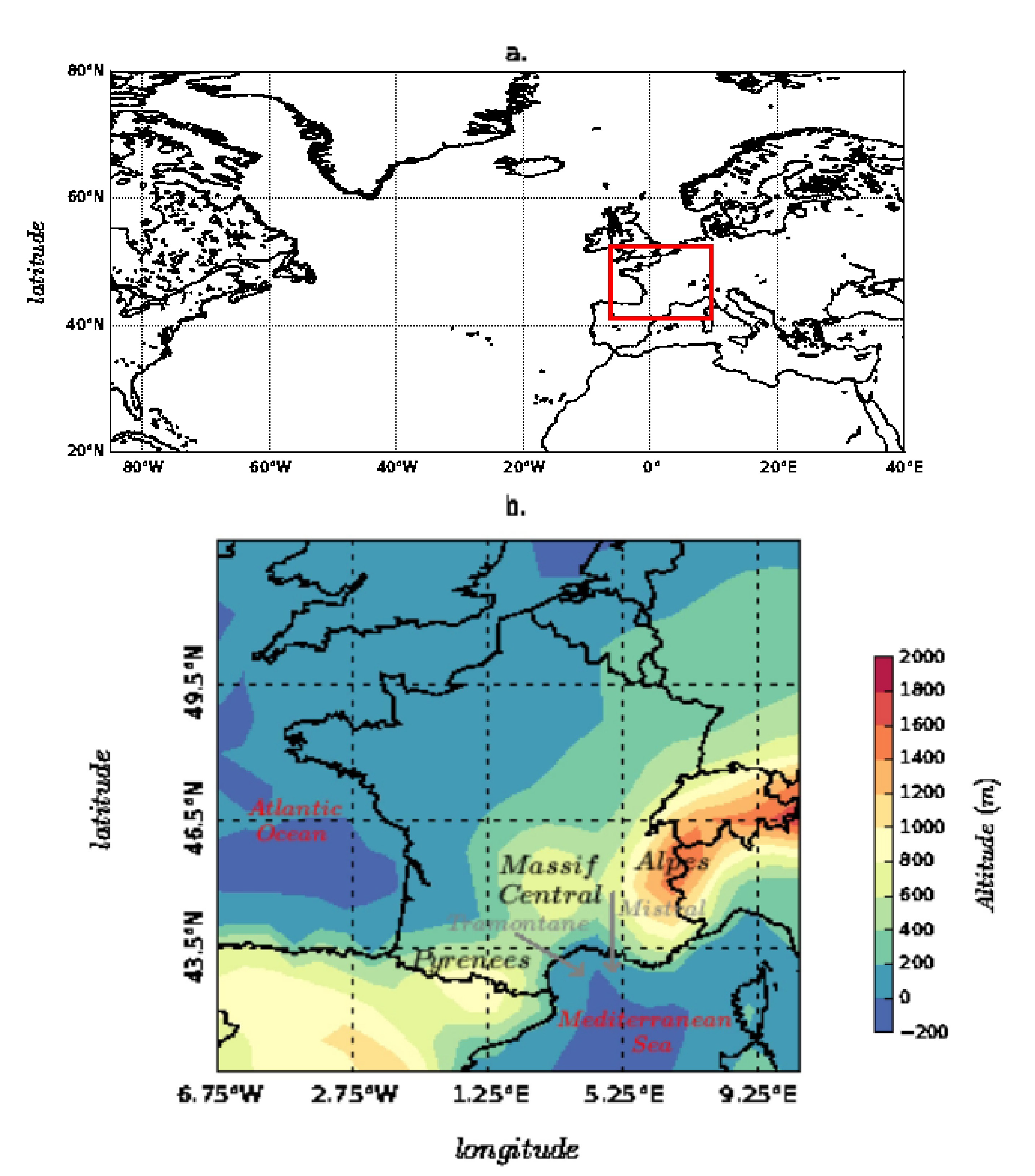
The 500-hPa geopotential height (Z500) is used to represent the large scale atmospheric circulation. Applying principal component analysis (PCA) to Z500, obtained over a large domain covering the North Atlantic/European region (Figure 2a), allows to reduce its dimensions and extract large-scale atmospheric circulation patterns which explain a large part of the climate variability over Europe. The outputs of the PCA are the empirical orthogonal functions (EOFs) describing the prevalent spatial patterns in the data, and the associated principal components (PCs) time series which show how the state of the atmosphere projects onto these patterns (Figure 3). In other words, denoting Z t ( x ) the 500-hPa geopotential height Z 500 on day t at the spatial location x, the PCA allows to reconstruct Z t ( x ) as:
Z t ( x ) = i = 1 n X t ( i ) f i ( x ) + E t ( x ) ,
where X t ( i ) are the PCs, f i ( x ) are the EOFs and E is the component which is not explained by the first n PCs. The quantity X t ( i ) are used as explanatory variables of the consumption and production and are gathered into two indexes ( I C o and I P r ) throught polynomial regression Equation (4).

2.2.2. Consumption ( C o ) and production ( P r )

The consumption value of interest is the daily consumption peak in fall and winter. The consumption peak at 7:00 pm C o is inferred here from the daily mean temperature in France T F (in °C). First, the temperature driven national mean consumption C o F expressed in GW is computed for winter and fall using the following relation:
C o F = 2.4 × ( 15 T F ) , if T F < 15 C . 0 , otherwise .
The national peak of consumption C o is then estimated as a linear regression of the national mean consumption C o F . In order to model the weekly variability of the consumption in France, we write the linear regression as follows:
C o = ( β c w C o F + I C w ) θ w ( t ) + ( β c o C o F + I C o ) θ o ( t )
with t the day of the year. And
θ w ( t ) = 1 if t is a working day . 0 , otherwise .
and
θ o ( t ) = 1 if t is a day off . 0 , otherwise .
We compute the national wind energy production P r 0 by applying a typical power curve (e.g., a power curve of Vestas V90-2.0 MW wind turbine which is one of the most deployed in France) to daily wind speed. A bias correction using a linear regression is then applied beween observed and computed production P r 0 :
P r = β P r P r 0 + I P r .

2.3. Calibration of the Model

Table 1 gives a summary of the data used in this study as well as of their transformation to obtain variables directly used in the model.
ERA-Interim (ERA-I) is a global atmospheric reanalysis performed by the European Center of Medium-range Weather Forecast (ECMWF) from 1 of January 1979 to 31 of August 2019. From ERA-I reanalysis, we retrieve the 500-hPa geopotential height ( Z 500 ) over the large domain (Figure 2a) (20 N to 80 N and 90 W to 40 E, with resolution 0.75 ). The time period considered in this study spans from 1 January 1979 to 31 December 2015. The data are available at 6-hour frequency, and are then averaged daily. After data averaging, we apply the PCA transformation to obtain the EOFs ( f i ) and PCs ( X ( i ) ). Figure 3 shows the three first EOFs and PCs. The first EOF ( f 1 ) and PC ( X ( 1 ) ) corresponds to the seasonal cycle (Figure 3a,b), explaining as much as 54.1% of the variance in the dataset. The following EOF ( f 2 ) and PC ( X ( 2 ) ) is related the North Atlantic Oscillation (NAO) (Figure 3c,d). The third EOF( f 3 ) and PC ( X ( 3 ) ) is related to the Scandinavian pattern (SCA) (Figure 3e,f).
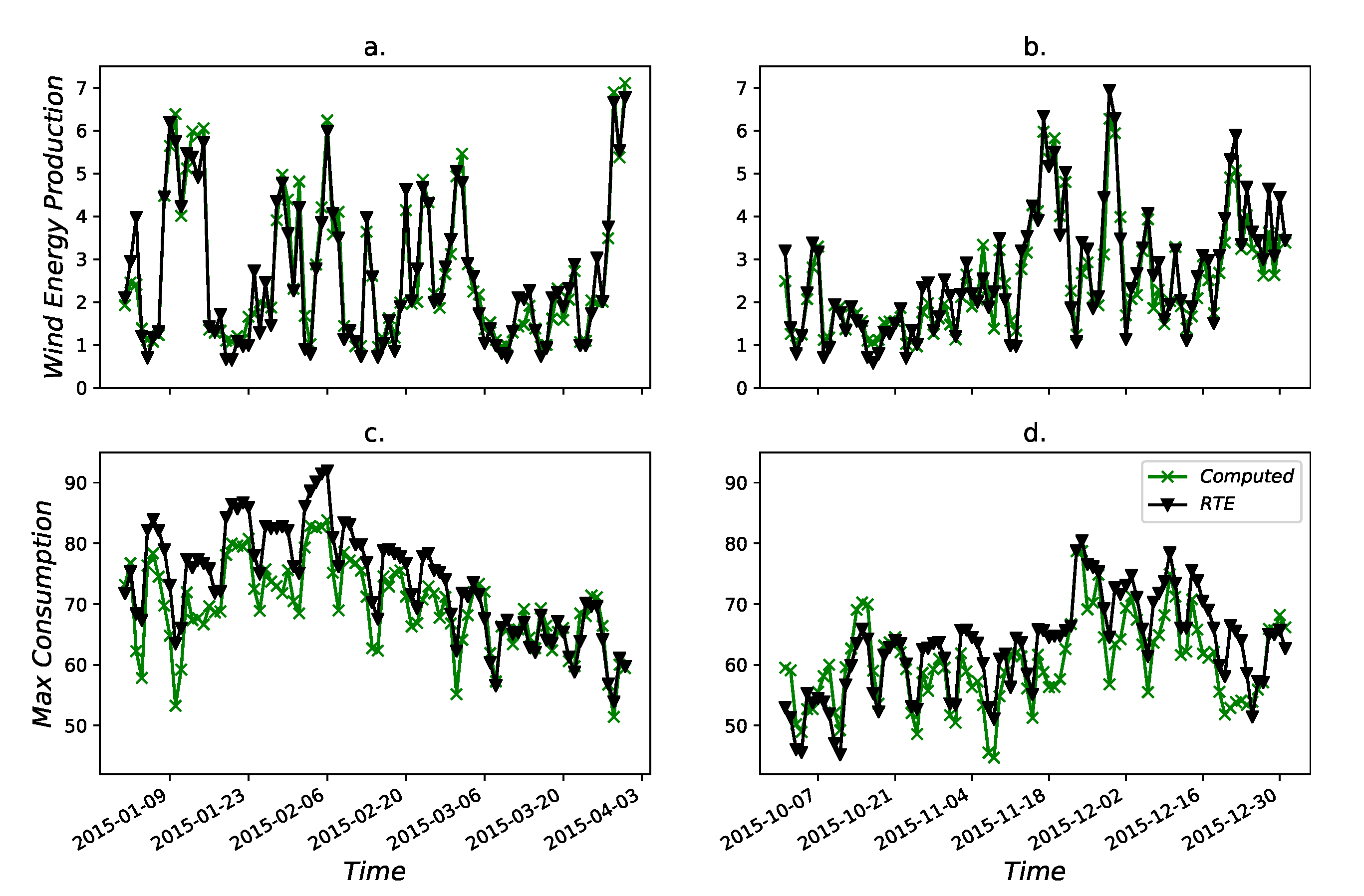
From ERA-I, we also retrieve the 10 m wind speed (which is extrapolated to 80 m height using the power law) and the 2 m temperature over the domain covering France (Figure 2b) (40.5 N to 52.5 N and −6.75 W to 10.5 E, with resolution 0.75 ). From the daily averaged data we compute the French daily wind energy production and peak of consumption. The parameters are calibrated with the hourly national consumption and wind energy production in 2015 retrieved from the French TSO Réseau de Transport d’Électricité (RTE) website (https://opendata.rte-france.com/). The consumption peak as well as the wind energy production thus correspond to the fixed electricity grid state in 2015. As a consequence, to adapt the model we need a good knowledge of the present electricity grid and wind installed capacity in France. Figure 4 shows the computed and measured wind energy production and consumption peak for winter and fall 2015.
We first define a period of 33 years between 1979 and 2011 to apply our model to ERA-I transformed data and to assess its accuracy for reconstructing risks of imbalance in a cross validation mode. Conditional PDF P ( P r , C o | I P r , I C o ) is estimated by KDE over 32 years and the joint PDF is reconstructed for the remaining year. We also estimate using KDE the real joint PDF for the remaning year. Doing this 33 times, we obtain 33 reconstructed and real joint PDF for winter and fall. A seasonal joint PDF of the climatology is estimated by KDE on the entire sample of 33 years, after checking that no significant variations can be found after removing one of the 33 years (stable climatology). So for each season among the 33 years, we obtain 3 joint PDFs, namely a climatology, a real joint PDF, and a forecasted joint PDF, as explained previously.
The years from 2012 to 2015 are kept for forecast purpose (Section 4). In order to forecast the joint distribution of P r and C o , we project the Z 500 field of each members of the ensemble onto the EOFs identified previously to obtain the PCs ( X i ). We compute the indexes I P r and I C o . By integrating the conditional distributions over the indexes and averaging through time, we obtain forecasted joint distribution at the monthly and seasonal horizon. Again, for each season and month of forecast, we obtain 3 distinct joint PDFs, a climatology, a real joint PDF, and a forecated joint PDF.

3. Model Performance Assessment

3.1. Modelling Results

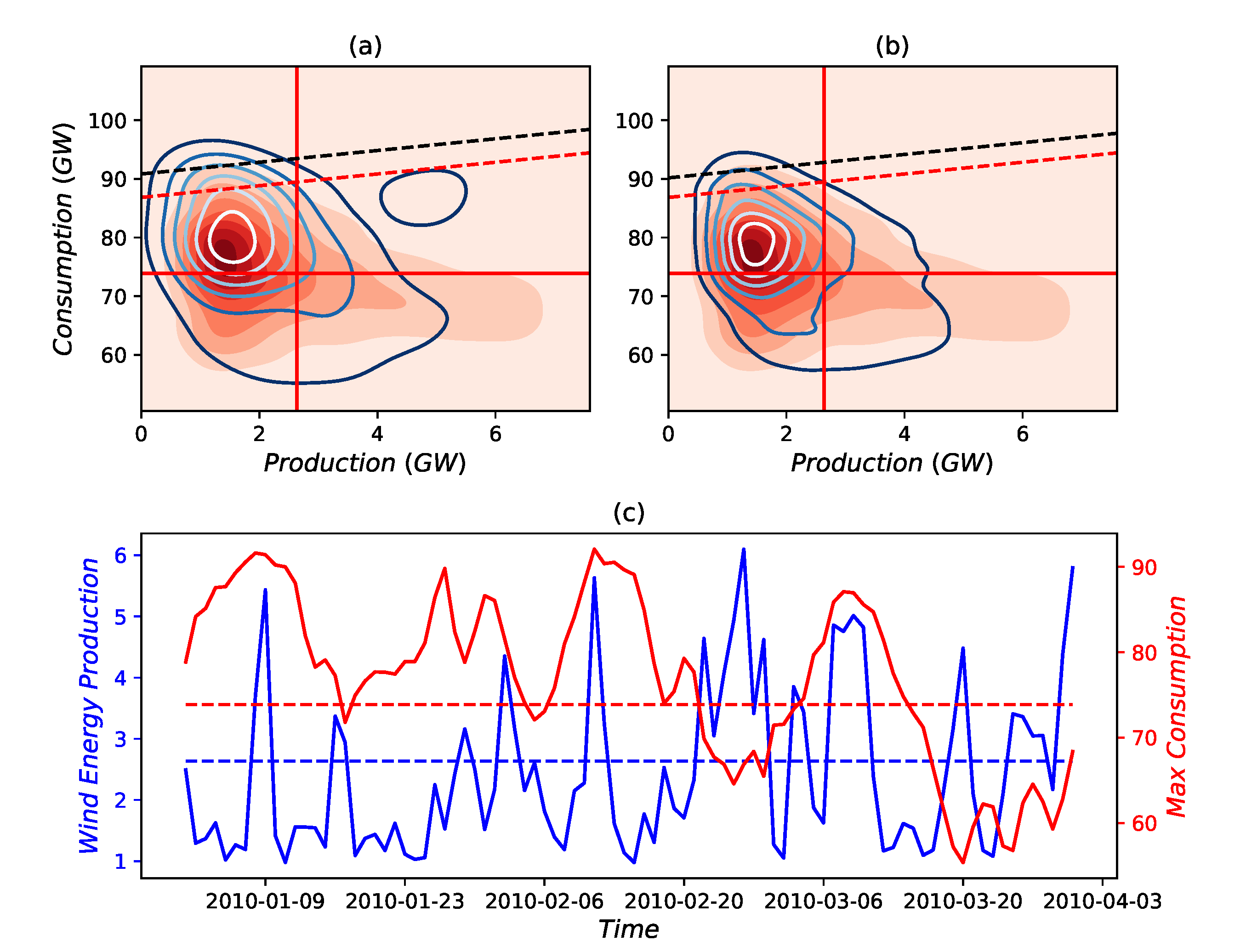
Figure 5 displays the real (contour lines, Figure 5a), reconstructed (contour lines, Figure 5b) and climatological (color shading) joint PDFs P ( P r , C o ) for winter 2010. The red vertical and horizontal lines correspond to the average production and consumption, respectively. They define the 4 quadrants as shown in Figure 1. The red dashed line correspond to the climatological V a R 95 of D c p and the black dashed lines correspond to the real (Figure 5a) and reconstructed (Figure 5b) V a R 95 of D c p . The model shows higher risk of high consumption and low production ( R c + p ) than normal. Indeed, deviation from the climatology is significant for both real and reconstructed PDFs. The maximum probability is well located by the reconstructed PDF and is located in the quadrant corresponding to R c + p . The real (Figure 5a) and reconstructed (Figure 5b) PDFs are very similar but the reconstructed PDFs is more peaked around the maximum probability in comparison to the real PDF.
Integrating the real and reconstructed PDFs over the quadrant corresponding to R c + p gives a risk of high consumption and low production 30% higher than the corresponding climatological risk. The V a R 95 r e a l for this winter is 90 GW while the climatological PDF gives a V a R 95 c l i m of 86GW. This means that there is a higher risk than normal to have situations of extreme imbalance. In other worlds, to secure the network 95% of the time, a TSO needs to plan a stock of 90 GW. The reconstructed PDF gives a good estimation of this risk as the V a R 95 r e c is of 90GW as well. Thus, the model representation of the joint PDF of production and consumption is satisfactory for this particular case of winter 2010. In Figure 5c, is displayed the time series of production (in blue) and consumption (in red) of winter 2010. It shows a 1.5 month period between 1 January and mid-February of higher consumption than normal (dashed red line) and lower production than normal (dashed blue line), during which stable anticyclonic conditions resulted in colder temperatures and weaker winds. During this period, production also displays peaks, associated with passing weather fronts, that helped satisfy the demand momentarily. On 20 February, consumption decreases while production sharply increases. This event only lasts 5 days and corresponds to a front passing over France bringing strong winds as well as warmer air from the South.
Performing a cross validation year by year over the period between 1979 and 2011 gives a time series of the risks of supply-demand imbalance for each season of each year. Figure 6 shows the time series of the real (in black) and reconstructed (in blue) risk measures compared with the climatological level of risk (in red). Figure 6a,b display the risks R c + p normalized by the climatology for winter and fall respectively and Figure 6c,d displays the opposite risks also normalized by the climatology R c p + . A value above (below) one indicates a higher (lower) risk than normal. Dashed red lines are thresholds corresponding to a significance level of 10% (see Appendix B). We compute the mean absolute error (MAE) as well as the coefficient of variatiation of the root mean square error (CV-RSME) between the normalized real and reconstructed risks (i.e. R r e a l / R c l i m and R r e c / R c l i m , respectively).
Let us note y = R r e a l / R c l i m and y ^ = R r e c / R c l i m . The MAE and CV-RSME can be written as follows:
M A E = 1 T t = 1 T | y t y ^ t |
C V ( R M S E ) = y y ^ ¯ 2 y ¯
The MAE ranges between 0.11 and 0.15 and the CV-RMSE ranges from 0.12 to 0.16. The correlation between the time series is always higher than 0.82 and is even 0.90 for R c p + in winter.
Over the 33 year-period, 26 winters display risk of high consumption and low production significantly different from the climatological risk ( R c + p , Figure 6a). Out of these 26 winters, 21 are reproduced by the model (81%), 9 of which correspond to a risk higher than normal. The model also produces 4 false alarms and 3 misses (1979, 1981 and 1984) of risk higher than normal. Over the 33 year-period, 27 winters display risk of low consumption and high production significantly different from the climatological risk ( R c p + , Figure 6b). Out of these 27 winters, 20 are reproduced by the model (74%). The model misses 2 risky winters in 1998 and 1999, and produces 1 false alarm. For a given year, there is no winter displaying risk of low consumption and high production and a risk of high consumption and low production at a time. During the fall season, Figure 6c,d display much less deviation from the climatological risk (9 for high consumption and low production and 11 for low consumption and high production). The model reproduces 56% of high consumption and low production situations and 82% of low consumption and high production situations.
Figure 6e,f display the timeseries of the real (in black) and reconstructed (in blue) V a R 95 for winter and fall respectively. The level of the V a R 95 quantified using the climatological PDFis displayed in red. Dashed red lines are thresholds corresponding to a significance level of 10% (see Appendix B). The MAE is 2.8 and 2.5 GW for winter and fall, respectively and the CV-RMSE is 4.2% and 3.8% for winter and fall, respectively. The correlation is 0.69 and 0.66 for winter and fall, respectively. The good correlation together with the relatively low error made by the model (3% of the climatological V a R 95 ) shows the advantage of using such method compared to the climatological approach. For several winters (Figure 6e) (e.g., 1985, 2003, 2005, or 2010), the model allows to better cover the extreme risk than when using the climatology. For other winters (e.g., 1984, 1989, 1990 or 2002), while the climatological approach overestimates the risk, the model allows to better adapt the stock of power needed to cover the extreme risk which is lower than normal. There is a low fraction (12% of years) of winters (i.e., 1980, 1981, 1997 and 2009) for which the model underestimates the extreme risk more than the climatological approach. In these two last cases, there might be a compromise to be done between a risk of underestimation of the V a R 95 by the model, and the probable overestimation of the V a R 95 by the climatology. For the fall (Figure 6f), the reconstructed V a R 95 shows a larger fraction (21% of years) of years when it underestimates the risk more than the climatology. More generally, the model shows a tendency for underestimating the extreme risk which may be dangerous for the network in cases when extreme situations indeed happen. Nevertheless, for several falls (e.g., 1980, 1990, 2001 or 2010), the model allows to better cover the extreme risk than when using the climatology as for winter.
In any case, the reconstructed risk measures display good correlation with real risk measures. The risk measures R c + p and R c p + go in opposite directions in most cases, while R c + p and the extreme risk measure V a R 95 coincide several times. Thus, using both reconstructed risk measures R c + p and V a R 95 can sometimes help validating the risk appearance.

3.2. Explanatory Value of the First PCs

Situations of high risk of supply-demand imbalance are generally associated with large-scale weather regimes, identified with the PCA analysis as the seasonal, NAO and SCA patterns (the 3 first dominant patterns are analyzed).
Figure 7 displays the winter distribution of the three first PCs used to compute the indexes, namely the seasonal pattern (Figure 7a,b), NAO (Figure 7c,d) and SCA (Figure 7e,f). Black distributions are computed using the entire dataset, while blue (red) distributions are computed over the seasons which display higher (lower) risk of imbalance than normal. For a risk of high consumption and low production ( R c + p ) higher than normal (Figure 7, red distribution, left column), the PC value of the seasonal pattern is less negative than normal, whereas it is more negative for the SCA and particularly NAO pattern which indicates a less marked pressure gradient between the Islandic low and the Azores high. Overall, such combination of PCs corresponds to a less marked southward shift of the pressure gradient that influences the position of the jet stream over the Atlantic Ocean which is in turn located more to the north than normal. It results in a less active storm track, with weaker fronts and storms bringing high wind speeds and warmer air over Europe. Interestingly, the distribution of the PC values associated with the SCA pattern displays two modes clearly associated with the two types of risk ( R c + p and R c p + ). The study of [25] shows that during negative phases of SCA pattern, the storm track activity is enhanced, but it is also shifted northward over Scotland, Denmark and Northern Germany. This is in agreement with [26] who shows that the NAO pattern is spatially modulated by the SCA pattern. It is also in agreement with less wind energy production than normal in France during SCA negative phase, especially in the north of France where a large part of the installed capacity is located. During the fall season, there is no evident signal in the distributions, probably due to the smaller number of cases deviating from the climatology.

4. Risk Forecasting

4.1. Integration over the Seasonal Ensemble Forecasts of the ECMWF

From the 51 members of the ECMWF seasonal forecasts ensemble we retrieve the Z 500 over the large domain (Figure 2a). An ensemble is a set of several deterministic forecasts—the members—which differ from their initial state: the initial state of the “control member” is designed using the last forecast together with the assimilation of all observations available; the initial state of the other members are slightly perturbed. This way, the ensemble represents the uncertainty which grows with the forecast horizon. At a given horizon, the ensemble gives a range of the possible states of the atmosphere, and allows to estimate probabilities. The ECMWF seasonal ensemble forecasts are available every month (on the first day) and gives forecasts up to 6 months. The time resolution is 6 h which we average daily in our case. Due to a major change (in November 2011) in the NWP model and assimilation system used by ECMWF, we limit our study to four years from January 2012 to December 2015. Consequently, 48 forecasts are available. Keeping only months of winter season, we keep 12 forecasts at monthly horizon and 4 forecasts at the seasonal horizon (i.e., 3 months). We do not address the forecasts for fall season, as the model assessment showed lower performance than for winter, as well as lower risk to deviate from climatology than in winter.
On each member of the ensemble, we apply the PCA transformation found previously in ERA-I. We thus obtain for each of the 51 members of the ensemble the 25 PCs used to compute the indexes I P r and I C o . We integrate the joint conditional PDFs given in Equation (6) over the ensemble of the computed indexes. We obtain the forecasted joint PDF of C o and P r at each timestep which we average to monthly and seasonal (i.e., 3-month) horizon to obtain the joint PDF for a given month and season.

4.2. Monthly and Seasonal Forecasts

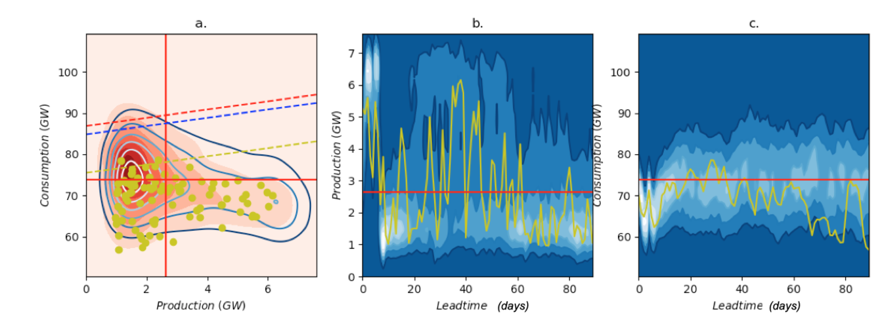
Figure 8 shows the forecast at the monthly horizon for January 2014 which is one of the well performing forecast in our small sample of forecasts. For this particular month, the risk of high consumption and low production ( R c + p ) is significantly below normal and is accurately predicted by our forecast. Indeed the consumption is between 10% and 25% below mean consumption. The risk of low consumption and high production ( R c p + ) is conversely higher than normal as low consumption is associated with wind energy production peaks. It is also well predicted by our forecast. The V a R 95 is also significantly below normal. Our forecast also predict a significantly lower V a R 95 than normal, but still overestimates the real V a R 95 by about 3 GW.
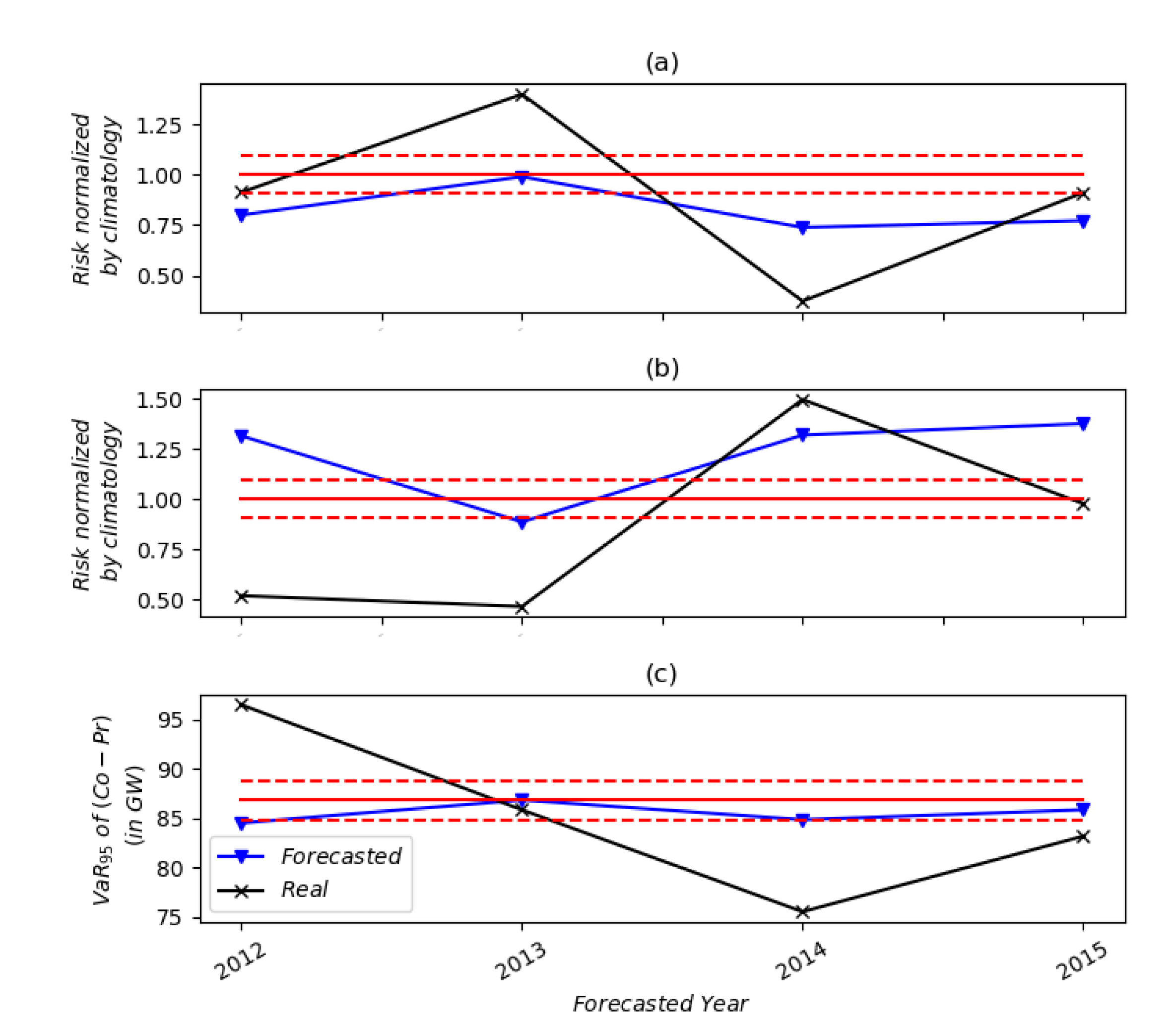
Figure 9 shows the forecasted (in blue) and real (in black) risks, i.e., the risk R c + p (Figure 9a), the risk R c p + (Figure 9b) and the extreme risk V a R 95 (Figure 9c) compared with the climatological risk (in red) for the first month of every 12 forecasts in winter. The correlations between the normalized real and forecasted risks are 0.54 and 0.82 for R c + p (Figure 9a) and R c p + (Figure 9b), respectively. Three occurrences of risk deviating from their climatological value are found for both high consumption and low production ( R c + p ) and low consumption and high production ( R c p + ). The correlation between the real and forecasted extreme risks is 0.65 for V a R 95 (Figure 9c). Nevertheless, despite the good correlation, the forecasted V a R 95 stays close to the climatological V a R 95 . The model gives only one false alarm in February 2015 indicating a significantly higher extreme risk than normal whereas the real extreme risk is in fact lower than normal. In all other cases, the model gives correct indications (or the same indication as the climatology), but with an error.
Figure 10 shows the seasonal forecasts for winter 2014 (from January to March). By comparison with monthly forecasts, the forecasted joint PDF is difficult to discern from the climatological joint PDF. The real values nevertheless seem to deviate from climatology as almost no values are in the top left quadrant. This can be seen when calculating the real risk R c + p normalized by the climatological risk (Figure 11a). For winter 2014, the real risk R c + p is much lower than 1, while the forecasted risk is close to 1. The same indication is given by the real and forecasted of the V a R 95 (Figure 11c).
This is not only the case for 2014, but for any winter and fall. The forecast seem to tend to the climatology (Figure 11). Contrary to monthly forecast, significance of this conclusion is difficult to assess because of the small number of samples.

5. Conclusions

In this study, three risk measures of supply-demand imbalance associated with wind energy production are defined. Two of them correspond to the risk of deviation from the climatological means of consumption and wind energy production. They are both quantified in terms of probability by integrating the joint probability of energy consumption and wind energy production in 2 quadrants. The other which corresponds to the extreme risk of supply-demand imbalance is the Value at Risk at 95% confidence level ( V a R 95 ) of the difference between consumption and production, quantified in GW. It is also derived from the joint probability of energy consumption and wind energy production. With such approach, the risk measures are compared to their climatological values.
To forecast the risks of supply-demand imbalance at monthly to seasonal time horizons, a statistical model is developed to reconstruct the joint probability of consumption and production. It is based on the conditional probability of production and consumption with respect to indexes obtained from a linear regression of principal components of large-scale atmospheric predictors.
For the first two risks, the reconstructed risk accurately reproduces the actual risk with over about 0.80 correlation in time (up to 0.90 in winter), and a hit rate around 70–80% (down to about 60% in fall for high consumption and low production risk). The accurate reconstruction, especially in winter, shows that the model is able to follow the interannual variations of consumption and production, in relation with large-scale weather pattern variability. For the extreme risk, the MAE is about 3% of the climatological risk, the CV-RMSE is about 4% of the mean actual V a R 95 and the correlation is 0.69 and 0.66 for winter and fall, respectively.
By applying our model to ensemble forecasts performed with a numerical weather prediction model, we show that forecasted risk measures up to 1 month horizon can outperform the climatology often used as the reference forecast (time correlation with actual risk ranging between 0.54 and 0.82). At seasonal time horizon (3 months), our forecasts seem to tend to the climatology. The small sample of seasonal forecasts used in the study nevertheless limits this conclusion.
Our study only accounts for weather driven variability of wind energy production and energy consumption (related to the temperature). The seasonal risk for energy systems also depends on other weather driven production sources (hydropower, solar energy) and on non-meteorological factors such as the availability of conventional power plants, long term storage capacity such as pumping power plants and power-to-gas, as well as calendar (hour of the day, day of the week, holidays) and socio-economic factors (e.g., economic growth, energy policies). As skills have been shown at least at monthly time horizon, this study is therefore a first step to a more integrated monthly to seasonal energy forecasting system.

Author Contributions

Conceptualization, B.A., P.D., P.T. and R.P.; methodology, B.A., P.D., P.T. and R.P.; software, B.A.; validation, B.A., P.D., P.T. and R.P.; formal analysis, B.A., P.D., P.T. and R.P.; investigation, B.A., P.D., P.T. and R.P.; resources, B.A., P.D., P.T. and R.P.; data curation, B.A.; writing—original draft preparation, B.A. and P.D.; writing—review and editing, B.A., P.D., P.T. and R.P.; visualization, B.A., P.D., P.T. and R.P.; supervision, P.D., P.T. and R.P.; project administration, P.D., P.T. and R.P.; funding acquisition, P.D. and P.T. All authors have read and agreed to the published version of the manuscript.

Funding

This research was funded by 3rd Programme d’Investissements d’Avenir [ANR-18-EUR-0006-02] and by the Foundation of Ecole polytechnique (Chaire “Défis Technologiques pour une Energie Responsable”). It was funded by the ANR project FOREWER (ANR-14-CE05-0028) and by the LABEX ECODEC (ANR-11 IDEX-0003/Labex Ecodec/ANR-11-LABX-0047).

Acknowledgments

This work has been carried out at the Energy4Climate Interdisciplinary Center (E4C) of IP Paris and Ecole des Ponts ParisTech. It was supported by 3rd Programme d’Investissements d’Avenir [ANR-18-EUR-0006-02] and by the Foundation of Ecole polytechnique (Chaire “Défis Technologiques pour une Energie Responsable”). It was supported by the ANR project FOREWER (ANR-14-CE05-0028). Financial support from the LABEX ECODEC (ANR-11 IDEX-0003/Labex Ecodec/ANR-11-LABX-0047) is gratefully acknowledged. The research of Peter Tankov has also benefited from the supportof the FIME Research Initiative.

Conflicts of Interest

The authors declare no conflict of interest. The funders had no role in the design of the study; in the collection, analyses, or interpretation of data; in the writing of the manuscript, or in the decision to publish the results.

Appendix A. Sensitivity of the Model to the Number of PCs Used to Fit the Indexes

We first build 6 models with the number of PCs used to fit both indexes ranging from 5 to 30 with increment 5. We compute the mean absolute error (MAE) between the real and reconstructed risks normalized by the climatological risk. Figure A1 displays the result of the sensitivity analysis. The minimal error is found for 20 PCs for the risk of high consumption and low production ( R c p + ) and 25 for the risk of low consumption and high production ( R c + p ) for winter and fall. However, the difference of MAE between 20 and 25 PCs is low (at most 10% difference). In the study, 25 PCs are therefore used to compute the two indexes for both R c p + and R c + p and any season.
Figure A1. Mean absolute error (MAE) between the real and reconstructed risks normalized by the climatological risk as a function of the number of PCs used to fit the indexes I P r and I C o in Equation (4).
Energies 13 04888 g0a1

Appendix B. Significance Levels for the Risk Measures

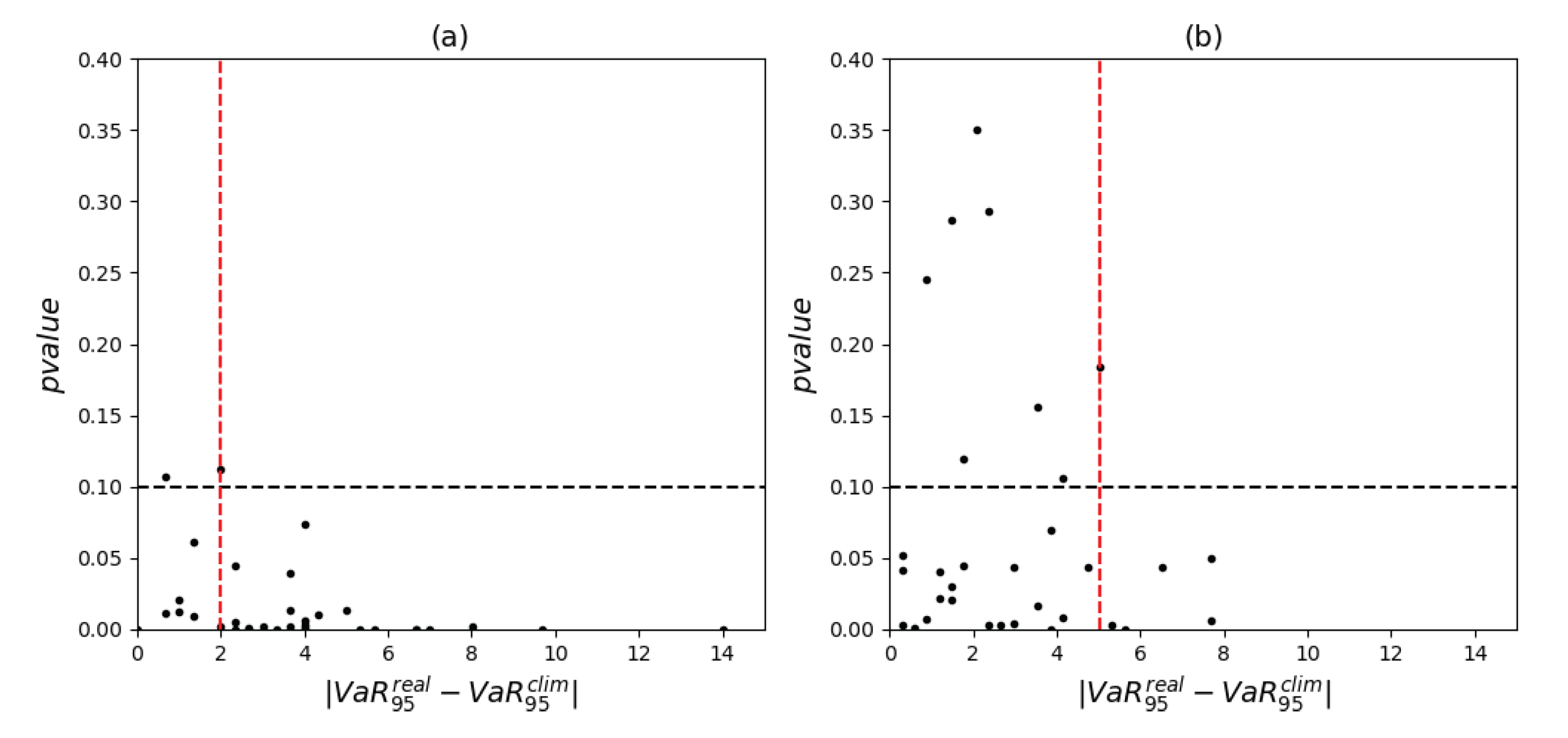
We perform a 2 dimensional Kolmogorov-Smirnov test [24] to test whether the real joint PDF and the climatological joint PDF are statistically identical or not. The p-value of the Kolmogorov-Smirnov test is then compared to the real risk measure normalized by its climatological value (Figure A2).
Figure A2. p-value resulting from the 2 dimensional Kolmogorov-Smirnov test performed between the climatological sample and the seasonal samples as a function of the real computed risk measure normalized by climatology. Black dashed line represents the 10% significance level for which the hypothesis of 2 samples coming from the same distribution cannot be rejected; Red dashed lines represent the threshold defined; (a) for winter and risk of high consumption and low production R c + p , (b) for winter and risk of low consumption and high production R c p + , (c) for fall and risk of high consumption and low production R c + p , (d) for fall and risk of low consumption and high production R c p + .
Energies 13 04888 g0a2
We consider the 10% significance level indicated with the black dashed line in Figure A2. Small p-values show that the 2 samples may not come from the same distribution, while high p-values show that the hypothesis that the seasonal joint PDF and the climatological joint PDF are identical cannot be rejected. Red dashed lines correspond to the thresholds for which we consider that the risk is significantly higher or lower than normal (climatology). They are defined by the largest deviation from 1 when the p-value is above significance levels of 10% (the value 1 corresponds to the climatological risk). This method is applied for both monthly and seasonal joint PDFs. The same method is applied to derive the significance levels for the extreme risk V a R 95 , as shown in Figure A3.
Figure A3. p-value resulting from the 2 dimensional Kolmogorov-Smirnov test performed between the climatological sample and the seasonal samples as a function of the absolute difference between the V a R 95 r e a l and V a R 95 c l i m . Black dashed line represents the 10% significance level for which the hypothesis of 2 samples coming from the same distribution cannot be rejected; Red dashed lines represent the threshold defined; (a) for winter, (b) for fall.
Energies 13 04888 g0a3

References

  1. RTE, Bilan électricique; RTE Report; Réseau de transport d’électricité de France: Paris, France, 2017.
  2. WindEurope. WindEurope, Wind Energy in Europe: Scenarios for 2030; Wind Europe Report; WindEurope: Brussels, Belgium, 2017. [Google Scholar]
  3. Alain Burtin and Vera Silva, Technical and Economic Analysis of the European Electricity System with 60% RES; EDF R&D Report; 2015. Available online: https://www.edf.fr/sites/default/files/Lot%203/CHERCHEURS/Portrait%20de%20chercheurs/summarystudyres.pdf (accessed on 6 August 2020).
  4. ENTSOE. ENTSOE, Winter Outlook Report—2016; ENTSOE Report; ENTSOE: Brussels, Belgium, 2016. [Google Scholar]
  5. RTE, Annual Electricity Report—2016; RTE Report; Réseau de transport d’électricité de France: Paris, France, 2016.
  6. Scaife, A.A.; Arribas, A.; Blockley, E.; Brookshaw, A.; Clark, R.T.; Dunstone, N.; Eade, R.; Fereday, D.; Folland, C.K.; Gordon, M.; et al. Skillful long-range prediction of European and North American winters. Geophys. Res. Lett. 2014, 41, 2514–2519. [Google Scholar] [CrossRef] [Green Version]
  7. Krakauer, N.Y.; Cohan, D.S. Interannual Variability and Seasonal Predictability of Wind and Solar Resources. Resources 2017, 6, 29. [Google Scholar] [CrossRef] [Green Version]
  8. Clark, R.T.; Bett, P.E.; Thornton, H.E.; Scaife, A.A. Skilful seasonal predictions for the European energy industry. Environ. Res. Lett. 2017, 12, 1–9. [Google Scholar] [CrossRef]
  9. Torralba, V.; Doblas-Reyes, F.J.; Macleod, D.; Christel, I.; Davis, M. Seasonal Climate Prediction: A New Source of Information for the Management of Wind Energy Resources. J. Appl. Meteorol. Climatol. 2017, 56, 1231–1247. [Google Scholar] [CrossRef]
  10. Soret, A.; Torralba, V.; Cortesi, N.; Christel, I.; Palma, L.; Manrique-Sunen, A.; Lledo, L.; Gonzalez-Reviriego, N.; Doblas- Reyes, F.J. Sub-seasonal to seasonal climate predictions for wind energy forecasting. J. Phys. Conf. Ser. 2019, 1222, 012009. [Google Scholar] [CrossRef]
  11. Alonzo, B.; Tankov, P.; Drobinski, P.; Plougonven, R. Probabilistic wind forecasting up to 3 months ahead using ensemble predictions for geopotential height. Int. J. Forecast. 2020, 36, 515–530. [Google Scholar] [CrossRef]
  12. Bett, P.E.; Thornton, H.E.; Troccoli, A.; De-Felice, M.; Suckling, E.; Dubus, L.; Saint-Drenan, Y.M.; Brayshaw, D.J. A Simplified Seasonal Forecasting Strategy, Applied to Wind and Solar Power in Europe. 2019. Available online: https://ideas.repec.org/p/osf/eartha/kzwqx.html (accessed on 2 February 2019).
  13. Lledo, L.; Torralba, V.; Soret, A.; Ramon, J.; Doblas-Reyes, F.J. Seasonal forecasts of wind power generation. Renew. Energy 2019, 143, 91–100. [Google Scholar] [CrossRef]
  14. Bett, P.E.; Thornton, H.E. The climatological relationships between wind and solar energy supply in Britain. Renew. Energy 2016, 87, 96–110. [Google Scholar] [CrossRef] [Green Version]
  15. Staffell, I.; Pfenninger, S. The increasing impact of weather on electricity supply and demand. Energy 2018, 145, 65–78. [Google Scholar] [CrossRef]
  16. de-Queiroz, A.R.; Mulcahy, D.; Sankarasubramanian, A.; Deane, J.P.; Mahinthakumar, G.; Lu, N.; DeCarolis, J.F. Repurposing an energy system optimization model for seasonal power generation planning. Energy 2019, 181, 1321–1330. [Google Scholar] [CrossRef] [Green Version]
  17. Parka, H.; Baldick, R. Optimal capacity planning of generation system integrating uncertain solar and wind energy with seasonal variability. Electr. Power Syst. Res. 2020, 180, 106072. [Google Scholar] [CrossRef]
  18. Schroeder, R.; Joyeau, A.; Carlini, E.M. Seasonal Adequacy Risks: Getting prepared for seasonal adequacy risks on regional level. In Proceedings of the IEEE international Conference on Environement and Electrical Engineering and IEEE Industrial and Comercial Power System Europe, Palermo, Italy, 12 June 2018; pp. 1–6. [Google Scholar]
  19. Orlov, A.; Silmann, J.; Vigo, I. Better seasonal forecasts for renewable energy industry. Nat. Energy 2020, 5, 108–110. [Google Scholar] [CrossRef]
  20. Prior, J.; Kendon, M. The UK winter of 2009/2010 compared with severe winters of the last 100 years. Weather 2011, 66, 4–10. [Google Scholar] [CrossRef]
  21. Brayshaw, D.J.; Dent, C.; Zachary, S. Wind generation’s contribution to supporting peak electricity demand - meteorological insights. Proc. Inst. Mech. Eng. Part O J. Risk Reliab. 2012, 226, 44–50. [Google Scholar] [CrossRef]
  22. Leahy, P.G.; Foley, A.M. Wind generation output during cold weather-driven electricity demand peaks in Ireland. Energy 2012, 39, 48–53. [Google Scholar] [CrossRef] [Green Version]
  23. Cradden, L.C.; McDermott, F. A weather regime characterisation of Irish wind generation and electricity demand in winters 2009–2011. Environ. Res. Lett. 2018, 13. [Google Scholar] [CrossRef]
  24. Fasano, G.; Franceschini, A. A multidimensional version of the Kolmogorov-Smirnov test. Mon. Not. R. Astron. Soc. 1986, 225, 155–170. [Google Scholar] [CrossRef]
  25. Bueh, C.; Nakamura, H. Scandinavian pattern and its climatic impact. Q. J. R. Meteorol. Soc. 2007, 133, 2117–2131. [Google Scholar] [CrossRef]
  26. Jourdier, B. Wind Resource in Metropolitan France: Assessment Methods, Variability and Trends. Ph.D. Thesis, Ecole Polytechnique, Palaiseau, France, 2015. [Google Scholar]
Figure 1. (a) Schematic of the joint distribution P ( C o , P r ) for a given season overlaid with the climatological production and consumption averages P r ¯ and C o ¯ displayed with the vertical and horizontal lines. The quantities C + , C , P + and P correspond to C o > C o ¯ , C o < C o ¯ , P r > P r ¯ and P r < P r ¯ , respectively. The quantities R c + p = P ( P r < P r ¯ , C o > C o ¯ ) and R c p + = P ( P r > P r ¯ , C o < C o ¯ ) correspond to risk of low production and high consumption and to risk of low consumption and high production, respectively. (b) Schematic of the joint distribution P ( C o , P r ) for a given season overlaid with the line of constant D c p = C o P r which separate the probability into a part where P ( C o , P r ) = 0.05 and another where P ( C o , P r ) = 0.95 . The corresponding quantity D c p = R 95 is the Value at Risk 95 ( V a R 95 ) of D c p
Energies 13 04888 g001
Figure 2. (a) North Atlantic/European domain from where the 500-hPa geopotential height Z 500 is retrieved. The red box corresponds to the domain in panel b. (b) Domain covering France and part of its neighbouring countries. The colors represents the topography and bathymetry.
Energies 13 04888 g002
Figure 3. First EOFs (left) and first five PCs (right) of the PCA performed on the fitting and validation period on the North Atlantic/Europe domain of ERA-Interim Z500 dataset. (a) EOF and (b) PC corresponding to the seasonal pattern. (c) EOF and (d) PC corresponding to North Atlantic Oscillation pattern. (e) EOF and (f) PC corresponding to Scandinavian pattern.
Energies 13 04888 g003
Figure 4. French daily wind energy production (a) in winter and (b) in fall 2015 from RTE data (in black) and computed using ERA-I surface wind speed (in green); and French daily maximum consumption (c) in winter and (d) in fall 2015 from RTE data (in black) and computed using ERA-I surface temperature (in green).
Energies 13 04888 g004
Figure 5. Blue contour lines show (a) the real and (b) the reconstructed joint PDF for winter 2010. Red shading show the winter climatological joint PDF. Red vertical and horizontal lines correspond respectively to the mean production and mean consumption given by climatology. Red dashed line shows the V a R 95 of C o P r given by the climatological joint PDF, black dashed lines show the V a R 95 of C o P r given by (a) the real and (b) the reconstructed joint PDF. (c) Time series of the wind energy production (in blue) and the temperature driven consumption (in red) during winter 2010. Dashed lines show the winter mean climatological value of the wind energy production (in blue) and of the consumption (in red).
Energies 13 04888 g005
Figure 6. Time series of the real (black curves) and reconstructed (blue curves) measures risk compared with the climatological level of risk (in red). (a) Risk R c + p in winter; (b) Risk R c + p in fall; (c) Risk R c p + in winter; (d) Risk R c p + in fall; (e) Risk V a R 95 in winter; (f) Risk V a R 95 in winter. For risks R c + p (panels a,b) and R c p + (panels c,d) the risk measure is normalized by the climatological risk so that a value above (below) one highlight a higher (smaller) risk than normal., while for the risks V a R 95 , the risk is measured in GW. Dashed dotted red lines correspond significance levels at 10% as defined in the Appendix B.
Energies 13 04888 g006
Figure 7. Winter distributions of the 3 first Principal Components corresponding to Figure 3. In each panel 3 distributions are plotted, the distribution of all winters (in black); the distribution of risk higher than normal (in red); the distribution of risk lower than normal (in blue). (a) distributions of the seasonal pattern PC corresponding to a risk of high consumption and low production ( R c + p ); (b) distributions of the seasonal pattern PC corresponding to a risk of a risk of low consumption and high production higher than normal ( R c p + ). (c,d) same as (a,b) for the NAO pattern. (e,f) same as (a,b) for the SCA pattern.
Energies 13 04888 g007
Figure 8. Forecast of January 2014 at the monthly horizon. (a) Reconstructed joint PDF (blue contour), real daily data (yellow dots) and the climatological PDF for January (red contour). (b) time series of the ensemble forecast of production (in blue contour) and of the real production (in yellow). (c) time series of the ensemble forecast of consumption (in blue contour) and of the real consumption (in yellow). The red line indicates the climatological value of production and consumption. The red, blue and yellow dashed lines indicate the extreme risk V a R 95 given by the climatology, the forecasted and the real PDFs respectively.
Energies 13 04888 g008
Figure 9. Monthly forecasted (blue) and real (black) risk relative to the climatology for winter months for (a) high consumption and low production ( R c + p ) and (b) low consumption and high production ( R c p + ) and (c) Extreme risk V a R 95 . Dashed red lines indicate significance levels at 10%.
Energies 13 04888 g009
Figure 10. Same as Figure 8 for winter 2014 and the 3-month forecast horizon (January to March).
Energies 13 04888 g010
Figure 11. Same as Figure 9 for winters at the 3-month forecast horizon (January to March).
Energies 13 04888 g011
Table 1. Summary of the data used for this study as well as of their transformation.
VariableData SourceTime PeriodTime ResolutionComputationResult
10 m
wind speed
ERA-I01-01-1979
31-12-2015
6-hourly- Averaged daily
- Compute Pr
Pr
(1979 to 2015)
French
Production
RTE01-01-2015
31-12-2015
hourly
2 m
temperature
ERA-I01-01-1979
31-12-2015
6-hourly- Averaged daily
- Average in France
- Compute Max Co
Co
(1979 to 2015)
French
consumption
RTE01-01-2015
31-12-2015
hourly
Z500ERA-I01-01-1979
31-12-2015
6-hourly- Averaged daily
- PCA
- Select several PCs
X 1 , , X n
(1979 to 2015)
Z500ECMWF seasonal
ensemble forecasts
01-01-2012
31-12-2015
6-hourly
Available
every month
- Averaged daily
- Apply PCA
- Select horizon
Ensemble of X n
(2012 to 2015)