Gini and Entropy-Based Spread Indexes for Primary Energy Consumption Efficiency and CO₂ Emission

Abstract

Primary energy consumption is one of the key drivers of global CO₂ emissions that, in turn, heavily depends on the efficiency of involved technologies. Either improvement in technology efficiency or the expansion of non-fossil fuel consumption requires large investments. The planning and financing of such investments by global policy makers or global energy firms require, in turn, reliable measures of associated global spread and their evolution in time, at least from the point of view of the principles for responsible investment (PRI). In this paper, our main contribution is the introduction of index measures for accessing global spread (that is, measures of inequality or inhomogeneity in the statistical distribution of a related quantity of interest) of technology efficiency and CO₂ emission in primary energy consumption. These indexes are based on the Gini index, as used in economical sciences, and generalized entropy measures. Regarding primary energy sources, we consider petroleum, coal, natural gas, and non-fossil fuels. Between our findings, we attest some stable relations in the evolution of global spreads of technology efficiency and CO₂ emission and a positive relation between changes in global spread of technology efficiency and use of non-fossil fuel.

1. Introduction

Primary energy sources are those directly found in nature and usable without any human engineered transformation. Global consumption of primary energy has been steadily increasing throughout human history; see [1] for a good account of the last decade. Hence, the efficiencies, in terms of CO₂ emission, of technologies used for primary energy consumption become key drivers of global CO₂ release [2]. There are different primary energy sources and several primary energy consumption technologies. Primary energy matrices and consumption technologies do vary from country to country and along time. Our first main contribution in this paper is to define appropriate index measures of global spread in efficiency, in terms of CO₂ emissions, for technologies used in primary energy consumption.

Primary energy sources are classified as fossil and non-fossil fuels. Fossil fuels comprise crude oil or petroleum, natural gas, and coal. These fuels come from theh remains of plants and animals buried millions of years ago and are, therefore, nonrenewable. Moreover the consumption of fossil fuels is responsible for most of the CO₂ release due to human activities. In contrast, non-fossil fuels comprise hydropower, biomass and biofuels, wind, geothermal, solar, nuclear (fission and fusion), and so on. Non-fossil fuels are in general renewable, with a few exceptions like fission nuclear fuels. Consequently, the spread of non-fossil fuels is a most welcome factor in mankind’s effort to reduce global CO₂ emissions. Our second main contribution in this paper is to define appropriate index measures of global spread in the use of non-fossil fuels.

Either the improvement of primary energy consumption technology efficiency, in terms of CO₂ emission, or the increase of non-fossil fuel consumption requires significant infrastructure adaptations and large public and private investments. We believe that our proposed index measures of global spread are useful tools in analysis and decision support that can benefit global policy makers and global energy sector firms. Since the global demand for energy has been increasing over the last decades and will continue to grow [3], long-term planning of investments in the energy matrix becomes of utmost importance [4,5,6,7,8,9,10].

Allocation of investments according to principles of responsible investment (PRI) requires objective measures. Our proposed index measures can provide global views and integrated perspectives of technology efficiency and non-fossil fuel use across different countries and the evolution of these scenarios over time. For instance, in a global carbon credit context, such measures could help to verify the effectiveness of policies for the regions buying or selling carbon credits in terms of decreasing the global spread of the technology efficiency and non-fossil fuel use over time. Furthermore, as market analysts and quantitative support experts for large Brazilian and international investment funds, it is the authors’ experience that the availability of good index measures of global spreads for energy consumption and efficiency can dramatically alter the perception and evaluation of investment opportunities in emerging markets. A more complete presentation, bringing graphical supporting tools and appropriate measures based on scientific facts, helps the decision akers and avoids possible misconceptions or prejudices due to lack of information.

In the context of economical sciences, the seminal work of Corrado Gini (1912) [11] introduced an income spread index measure referred to in the literature as the Gini index. The Gini index measures the equality or inequality (homogeneity or inhomogeneity) of income distribution per capita. The Gini index has already been used to measure either the spread of the CO₂ emissions per capita [12,13,14,15] or the spread of energy consumption per capita [16]. There are other applications of the Gini index related to electricity consumption [17] or resource inequalities in a broader context [18]. However, it is important to stress that, in the present paper, differently from [17] or [18], our focus is on the introduction of index measures for accessing global spreads of technology efficiency in terms of CO₂ emission and non-fossil fuel use. In particular, Soares et al. (2018) [19] have compared the technology efficiency of different countries using clustering techniques based on the Gini index of CO₂ emissions per capita and presented subsequent comparative analyses of such clusters. In this paper, our approach is substantially different; it does not rely on group comparisons and, hence, does not depend on additional criteria used for intermediate cluster formation.

An alternative to the Gini index is entropy indexes conceived to generalize some spread measures like the mean log deviation, Atkinson index, Theil index, etc.; see [20,21,22,23]. According to Bourguignon (1979) [21], a good spread index should have the property of additive decomposability, that is, it should provide a measure such that the total spread of a population can be broken down into a weighted average of spreads within subgroups of the same population. Unfortunately, the Gini index is not additively decomposable, motivating the construction of more suitable indexes in this respect, like generalized entropy indexes.

This paper is organized as follows: Section 2 presents details of our proposed methodologies to measure global spread in efficiencies of technologies used for primary energy consumption or to measure global spread in the use of non-fossil fuels. Section 3 presents an empirical study, describing the utilized data and exemplifying the use of the Gini and the generalized entropy index. Section 4 gives our final conclusions.

2. Methodologies

In this section, we define the efficiency measures used in this paper for primary energy consumption technology. In addition, we present our proposed methodologies to measure global spreads of these quantities based on the Gini index and the generalized entropy index. We introduce the following notations: $e_{n,t}^m$ is the CO₂ emission of country n derived from consumption of primary energy source m during time interval t (e.g., MM Tons of CO₂); $c_{n,t}^m$ is the consumption of country n of primary energy m during time interval t (e.g., quad-BTU); $n\in \left\{1,\dots ,N\right\}$; $m\in \left\{1,\dots ,M\right\}$; $t\in \left\{1,\dots ,T\right\}$; N is the number of countries; M is the number of primary energies; and T is the number of time intervals.

2.1. Efficiencies in Primary Energy Consumption Technologies in Terms of CO₂ Emissions

We define the efficiencies in primary energy consumption technology in terms of CO₂ emissions as follows:

$${\epsilon }_{n,t}^m=\frac{c_{n,t}^m}{e_{n,t}^m}.$$

(1)

The technology efficiency ${\epsilon }_{n,t}^m$ is an intensive variable, and consequently, it does not depend on the countries’ size, population, or gross domestic product. In contrast, the consumptions $c_{n,t}^m$ and the CO₂ emissions $e_{n,t}^m$ are extensive variables, depending on the countries’ size. Notice that, for a fixed $e_{n,t}^m$, the technology efficiency ${\epsilon }_{n,t}^m$ is higher when $c_{n,t}^m$ is higher and vice versa. For a fixed $c_{n,t}^m$, the technology efficiency ${\epsilon }_{n,t}^m$ is higher when $e_{n,t}^m$ is lower and vice versa.

According to Lawrence et al. (2013) [16], issues of total energy consumption and CO₂ emission are inextricably related to problems of energy inequality among countries, and the study of those issues constitute one of the main motivations for this paper. However, Lawrence et al. (2013) [16] focus on the distribution among countries of the total energy consumption per capita (dividing the total energy consumption per unit time in each country by its population), implicitly assuming that this quantity can be automatically linked to CO₂ emission. An important contribution of this paper is to include our efficiency measures in this analysis, leading to more accurate perspectives of CO₂ emission. Moreover, our efficiency measures are also specific for each primary energy consumption technology, hence allowing even more detailed views of energy consumption and its relations to CO₂ emissions.

In [16], the authors argue for the convenience of using complementary distribution functions of the population parameterized by the total energy consumption per capita rather than the corresponding probability density function because of the discrete number of countries in the world and the fact that it is a more sensible approach to assign weights to different countries proportional to their populations to avoid a group of tiny countries outweighing the few most populous countries (for a more detailed description of the underlying concepts, see Milanović (2007), [24]). Analogoulsy, for our efficiency measures, it is also a more sensible approach to assign weights to different countries proportional to their CO₂ emissions. As far as we know, our study is the first, among similar studies, focusing primarily on the global probability density function, $f_{{\epsilon }_t^m}\left(·\right)$, and the global complementary cumulative distribution function, ${\overline{F}}_{{\epsilon }_t^m}\left(·\right)$, of CO₂ emissions parameterized by the technology efficiency, ${\epsilon }_t^m$.

By definition, the relationship between ${\overline{F}}_{{\epsilon }_t^m}\left(·\right)$ and $f_{{\epsilon }_t^m}\left(·\right)$ is

$${\overline{F}}_{{\epsilon }_t^m}\left(\epsilon \right)={\int }_{\epsilon }^{\infty }{f}_{{\epsilon }_t^m}\left(z\right)dz.$$

(2)

The corresponding Lorenz curve is defined as a parametric bidimensional plot having

$$x_{{\epsilon }_t^m}\left(\epsilon \right)=1-{\overline{F}}_{{\epsilon }_t^m}\left(\epsilon \right)={\int }_0^{\epsilon }{f}_{{\epsilon }_t^m}\left(z\right)dz$$

(3)

as its abscissa and

$$y_{{\epsilon }_t^m}\left(\epsilon \right)=\frac{1}{〈{\epsilon }_t^m〉}{\int }_0^{\epsilon }z{f}_{{\epsilon }_t^m}\left(z\right)dz,$$

(4)

as its ordinate. Moreover, $\epsilon$ goes from 0 to ∞ and

$$〈{\epsilon }_t^m〉={\int }_0^{\infty }z{f}_{{\epsilon }_t^m}\left(z\right)dz$$

(5)

is the global technology efficiency for the consumption of the primary energy m at the time interval t. This definition for the Lorenz curve is based on [16,22]. Notice that, since the values $x_{{\epsilon }_t^m}\left(\epsilon \right)$ and $y_{{\epsilon }_t^m}\left(\epsilon \right)$ are bounded between zero and one, the Lorenz curve always connects the points $\left(0,0\right)$ and $\left(1,1\right)$.

Considering weights to different countries proportional to their CO₂ emissions, our empirical estimator of the global complementary cumulative distribution function of the CO₂ emissions parameterized by the technology efficiency is given by the following (for analytical details for an analogous case, see [16,24]):

$${\widehat{\overline{F}}}_{{\epsilon }_t^m}\left({\tilde{\epsilon }}_{n,t}^m\right)=\frac{{\sum }_{i=n+1}^N{\tilde{e}}_{i,t}^m}{{\sum }_{i=1}^N{\tilde{e}}_{i,t}^m},\forall n\in \left\{1,\dots ,N\right\},$$

(6)

where the ordered set

$$\left\{{\tilde{\epsilon }}_{1,t}^m,\dots ,{\tilde{\epsilon }}_{N,t}^m\right\}$$

(7)

is obtained by sorting the set

$$\left\{{\epsilon }_{1,t}^m,\dots ,{\epsilon }_{N,t}^m\right\}$$

(8)

in the ascending order and by the same country order is applied to the sets

$$\left\{e_{1,t}^m,\dots ,e_{N,t}^m\right\}\mathrm{and}\left\{c_{1,t}^m,\dots ,c_{N,t}^m\right\}$$

(9)

to obtain, respectively, the ordered sets

$$\left\{{\tilde{e}}_{1,t}^m,\dots ,{\tilde{e}}_{N,t}^m\right\}\mathrm{and}\left\{{\tilde{c}}_{1,t}^m,\dots ,{\tilde{c}}_{N,t}^m\right\}.$$

(10)

For instance, ${\tilde{\epsilon }}_{1,t}^m=min\left\{{\epsilon }_{1,t}^m,\dots ,{\epsilon }_{N,t}^m\right\}$ and ${\tilde{\epsilon }}_{N,t}^m=max\left\{{\epsilon }_{1,t}^m,\dots ,{\epsilon }_{N,t}^m\right\}$.

Since the empirical global technology efficiency for consumption of primary energy m at time interval t is

$$〈{\widehat{\epsilon }}_t^m〉=\frac{{\sum }_{i=1}^N{\tilde{c}}_{i,t}^m}{{\sum }_{i=1}^N{\tilde{e}}_{i,t}^m}=\frac{{\sum }_{i=1}^N{c}_{i,t}^m}{{\sum }_{i=1}^N{e}_{i,t}^m},$$

(11)

it follows that

$${\widehat{x}}_{{\epsilon }_t^m}\left({\tilde{\epsilon }}_{n,t}^m\right)=\frac{{\sum }_{i=1}^n{\tilde{e}}_{i,t}^m}{{\sum }_{i=1}^N{\tilde{e}}_{i,t}^m} \mathrm{and} {\widehat{y}}_{{\epsilon }_t^m}\left({\tilde{\epsilon }}_{n,t}^m\right)=\frac{{\sum }_{i=1}^n{\tilde{c}}_{i,t}^m}{{\sum }_{i=1}^N{\tilde{c}}_{i,t}^m}.$$

(12)

Using both ${\widehat{x}}_{{\epsilon }_t^m}\left({\tilde{\epsilon }}_{n,t}^m\right)$ and ${\widehat{y}}_{{\epsilon }_t^m}\left({\tilde{\epsilon }}_{n,t}^m\right)$, it is possible to plot the corresponding empirical Lorenz curve.

The Gini index is a measure of statistical dispersion introduced by Corrado Gini in 1912 [11] to measure the income equality/inequality in a population. Using the Lorenz curve for technology efficiency, we define the Gini index of global spread of primary energy consumption technology efficiency in terms of CO₂ emissions (technology efficiency Gini index) as follows:

$$G_{{\epsilon }_t^m}={\mathcal{A}}_{{\epsilon }_t^m}/{\mathcal{B}}_{{\epsilon }_t^m}.$$

(13)

Considering the aforementioned $x_{{\epsilon }_t^m}\left(\epsilon \right)$ vs. $y_{{\epsilon }_t^m}\left(\epsilon \right)$ plot, ${\mathcal{A}}_{{\epsilon }_t^m}$ is the area between the line connecting the points $\left(0,0\right)$ and $\left(1,1\right)$ and the Lorenz curve and ${\mathcal{B}}_{{\epsilon }_t^m}$ is the area of the triangle formed by the points $\left(0,0\right)$, $\left(1,1\right)$, and $\left(0,1\right)$. Since ${\mathcal{B}}_{{\epsilon }_t^m}=0.5$, it follows that $G_{{\epsilon }_t^m}=2{\mathcal{A}}_{{\epsilon }_t^m}$. In addition, $0\le G_{{\epsilon }_t^m}\le 1$, with zero representing an equal global spread of the technology efficiency and 1 representing the highest possible inequality spread of the technology efficiency.

As an alternative to the Gini index, the generalized entropy index was introduced as a measure of income equality/inequality in a population [20]. We define the global spread of primary energy consumption technology efficiency index, in terms of CO₂ emissions, based on the generalized entropy measure (technology efficiency generalized entropy index) as follows:

$$E_{{\epsilon }_t^m}^{\alpha }=\left\{\begin{array}{cc}\frac{1}{N\alpha \left(\alpha -1\right)}\sum _{i=1}^N \left[{\left(\frac{{\epsilon }_{i,t}^m}{{\overline{\epsilon }}_t^m}\right)}^{\alpha }-1\right] ,\hfill & \alpha \notin \left\{0,1\right\},\hfill \\ -\frac{1}{N}\sum _{i=1}^{N}ln\frac{{\epsilon }_{i,t}^m}{{\overline{\epsilon }}_t^m},\hfill & \alpha =0,\hfill \\ \frac{1}{N}\sum _{i=1}^N\frac{{\epsilon }_{i,t}^m}{{\overline{\epsilon }}_t^m}ln\frac{{\epsilon }_{i,t}^m}{{\overline{\epsilon }}_t^m},\hfill & \alpha =1,\hfill \end{array}\right..$$

(14)

$\alpha$ is a real number and ${\overline{\epsilon }}_t^m$ is the mean value of ${\epsilon }_{i,t}^m,i=1,\dots ,N$. The values of $E_{{\epsilon }_t^m}^{\alpha }$ go from 0 to ∞, with zero representing an equal global spread of the technology efficiency and higher values representing higher inequality of technology efficiency spread. The values $\alpha =0$ and $\alpha =1$ are of particular interest, namely, $E_{{\epsilon }_t^m}^0$ is the technology efficiency mean log deviation index and $E_{{\epsilon }_t^m}^1$ is the technology efficiency Theil index.

The Atkinson index was introduced by Atkinson (1970) [23], and it can be derived from the generalized entropy index as follows. We define the global spread of the primary energy consumption technology efficiency based on the Atkinson index (technology efficiency Atkinson index) as follows:

$$A_{{\epsilon }_t^m}^{ϵ}=\left\{\begin{array}{cc}1-\frac{1}{{\overline{\epsilon }}_t^m} {\left[\frac{1}{N}\sum _{i=1}^N{\left({\epsilon }_{i,t}^m\right)}^{1-ϵ}\right]}^{1/\left(1-ϵ\right)} , \hfill & 0\le ϵ\ne 1,\hfill \\ 1-\frac{1}{{\overline{\epsilon }}_t^m}{\left(\prod _{i=1}^N{\epsilon }_{i,t}^m\right)}^{1/N},\hfill & ϵ=1,\hfill \end{array}\right..$$

(15)

$ϵ$ is called the inequality aversion parameter, since $A_{{\epsilon }_t^m}^{ϵ}$ becomes more sensitive to changes at the lower end of the technology efficiency distribution as $ϵ$ approaches 1 and $A_{{\epsilon }_t^m}^{ϵ}$ becomes more sensitive to changes in the upper end of the technology efficiency distribution as $ϵ$ approaches 0.

2.2. Non-Fossil Fuel Use

The non-fossil fuel use of a country n during the time interval t is defined as follows:

$${\rho }_{n,t}=\frac{c_{n,t}^{\star }}{c_{n,t}},$$

(16)

where $c_{n,t}^{\star }$ is the non-fossil fuel consumption of country n during the time interval t and $c_{n,t}$ is the total primary energy consumption of country n during the time interval n, i.e., $c_{n,t}={\sum }_{i=1}^M{c}_{n,t}^i$. Notice that the non-fossil fuel use ${\rho }_{n,t}$ is an intensive variable. As far as we know, our study is the first, among similar studies, focusing primarily on the global complementary cumulative distribution function ${\overline{F}}_{{\rho }_t}\left(·\right)$ of the total primary energy consumption parameterized by the non-fossil fuel use, ${\rho }_t$.

We define the empirical estimator

$${\widehat{\overline{F}}}_{{\rho }_t}\left({\tilde{\rho }}_{n,t}\right)=\frac{{\sum }_{i=n+1}^N{\tilde{c}}_{i,t}}{{\sum }_{i=1}^N{\tilde{c}}_{i,t}},\forall n\in \left\{1,\dots ,N\right\},$$

(17)

where the ordered set

$$\left\{{\tilde{\rho }}_{1,t},\dots ,{\tilde{\rho }}_{N,t}\right\}$$

(18)

is obtained sorting the set

$$\left\{{\rho }_{1,t},\dots ,{\rho }_{N,t}\right\}$$

(19)

in the ascending order, and using the same country order, we obtain

$$\left\{c_{1,t},\dots ,c_{N,t}\right\}\mathrm{and}\left\{c_{1,t}^{\star },\dots ,c_{N,t}^{\star }\right\}$$

(20)

$$\left\{{\tilde{c}}_{1,t},\dots ,{\tilde{c}}_{N,t}\right\}\mathrm{and}\left\{{\tilde{c}}_{1,t}^{\star },\dots ,{\tilde{c}}_{N,t}^{\star }\right\}.$$

(21)

Moreover, since the empirical global non-fossil fuel use at the time interval t is

$$〈{\widehat{\rho }}_t〉=\frac{{\sum }_{i=1}^N{\tilde{c}}_{i,t}^{\star }}{{\sum }_{i=1}^N{\tilde{c}}_{i,t}}=\frac{{\sum }_{i=1}^N{c}_{i,t}^{\star }}{{\sum }_{i=1}^N{c}_{i,t}},$$

(22)

it follows that

$${\widehat{x}}_{{\rho }_t}\left({\tilde{\rho }}_{n,t}\right)=\frac{{\sum }_{i=1}^n{\tilde{c}}_{i,t}}{{\sum }_{i=1}^N{\tilde{c}}_{i,t}} \mathrm{and} {\widehat{y}}_{{\rho }_t}\left({\tilde{\rho }}_{n,t}\right)=\frac{{\sum }_{i=1}^n{\tilde{c}}_{i,t}^{\star }}{{\sum }_{i=1}^N{\tilde{c}}_{i,t}^{\star }}.$$

(23)

Using both ${\widehat{x}}_{{\rho }_t}\left({\tilde{\rho }}_{n,t}\right)$ and ${\widehat{y}}_{{\rho }_t}\left({\tilde{\rho }}_{n,t}\right)$, it is possible to plot the corresponding empirical Lorenz curve.

Using the Lorenz curve for the non-fossil fuel use, we define the global spread of the non-fossil fuel use based on the Gini index (non-fossil fuel use Gini index) as follows:

$$G_{{\rho }_t}={\mathcal{A}}_{{\rho }_t}/{\mathcal{B}}_{{\rho }_t}.$$

(24)

Considering the $x_{{\rho }_t}\left(\rho \right)$ vs. $y_{{\rho }_t^m}\left(\rho \right)$ plot, ${\mathcal{A}}_{{\rho }_t^m}$ is the area between the line connecting the points $\left(0,0\right)$ and $\left(1,1\right)$ and the corresponding Lorenz curve and ${\mathcal{B}}_{{\rho }_t}$ is the area of the triangle formed by the points $\left(0,0\right)$, $\left(1,1\right)$ and $\left(0,1\right)$. Since ${\mathcal{B}}_{{\rho }_t}=0.5$, it follows that $G_{{\rho }_t}=2{\mathcal{A}}_{{\rho }_t}$. Moreover, $0\le G_{{\rho }_t}\le 1$, with zero representing a homogeneous global spread of the non-fossil fuel use and 1 representing the most inhomogeneous spread possible for non-fossil fuel use.

Analogously, for the technology efficiency generalized entropy index, we define the global spread of non-fossil fuel use based on the generalized entropy index (non-fossil fuel generalized entropy index) as follows:

$$E_{{\rho }_t}^{\alpha }=\left\{\begin{array}{cc}\frac{1}{N\alpha \left(\alpha -1\right)}\sum _{i=1}^N \left[{\left(\frac{{\rho }_{i,t}}{{\overline{\rho }}_t}\right)}^{\alpha }-1\right] ,\hfill & \alpha \notin \left\{0,1\right\},\hfill \\ -\frac{1}{N}\sum _{i=1}^{N}ln\frac{{\rho }_{i,t}}{{\overline{\rho }}_t},\hfill & \alpha =0,\hfill \\ \frac{1}{N}\sum _{i=1}^N\frac{{\rho }_{i,t}}{{\overline{\rho }}_t}ln\frac{{\rho }_{i,t}}{{\overline{\rho }}_t},\hfill & \alpha =1,\hfill \end{array}\right..$$

(25)

where $\alpha$ is a real number and ${\overline{\rho }}_t$ is the mean value of ${\rho }_{i,t},i=1,\dots ,N$. The values of $E_{{\rho }_t}^{\alpha }$ goes from 0 to ∞, with zero representing an equal global spread of non-fossil fuel use and higher values representing higher inequality spreads of non-fossil fuel use. Of particular interest are the values $\alpha =0$ and $\alpha =1$: $E_{{\rho }_t}^0$ is the non-fossil fuel mean log deviation index, and $E_{{\rho }_t}^1$ is the non-fossil fuel Theil index.

Analogously, for the technology efficiency Atkinson index, we define the non-fossil fuel Atkinson index as follows:

$$A_{{\rho }_t}^{ϵ}=\left\{\begin{array}{cc}1-\frac{1}{{\overline{\rho }}_t} {\left[\frac{1}{N}\sum _{i=1}^N{\left({\rho }_{i,t}\right)}^{1-ϵ}\right]}^{1/\left(1-ϵ\right)} ,\hfill & 0\le ϵ\ne 1,\hfill \\ 1-\frac{1}{{\overline{\rho }}_t}{\left(\prod _{i=1}^N{\rho }_{i,t}\right)}^{1/N},\hfill & ϵ=1,\hfill \end{array}\right..$$

(26)

The scalar $ϵ$ is known as the inequality aversion parameter, since $A_{{\rho }_t}^{ϵ}$ becomes more sensitive to changes at the lower end of the non-fossil fuel use distribution as $ϵ$ approaches 1 and $A_{{\rho }_t}^{ϵ}$ becomes more sensitive to changes in the upper end of the non-fossil fuel use distribution as $ϵ$ approaches 0.

3. Results and Discussion

This section illustrates the use of our proposed methodology using the US Energy Information Administration (EIA) data [25] from 1980 to 2015, for a set of 41 countries (Albania, Argentina, Australia, Austria, Bangladesh, Belgium, Brazil, Bulgaria, Burma, Canada, Chile, China, Colombia, Egypt, Finland, France, Hungary, India, Indonesia, Iran, Ireland, Italy, Japan, Luxembourg, Malaysia, Mexico, Morocco, Netherlands, New Zealand, Nigeria, Norway, Pakistan, Peru, Romania, Spain, Switzerland, Taiwan, Tunisia, United Kingdom, United States, and Venezuela). Countries were selected using criteria of data availability for the time period under consideration. Consumptions and emissions data are in quad-BTU and MM Tons of CO₂, respectively.

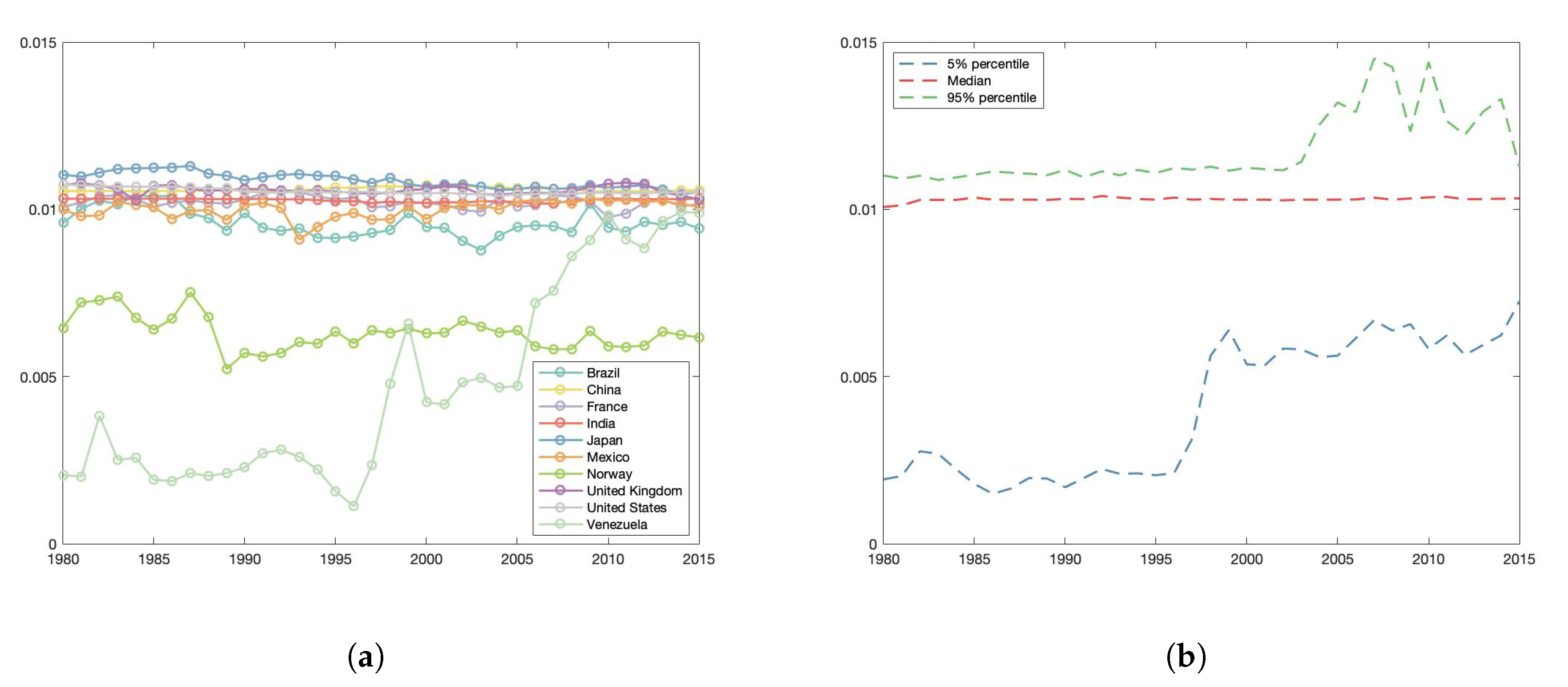
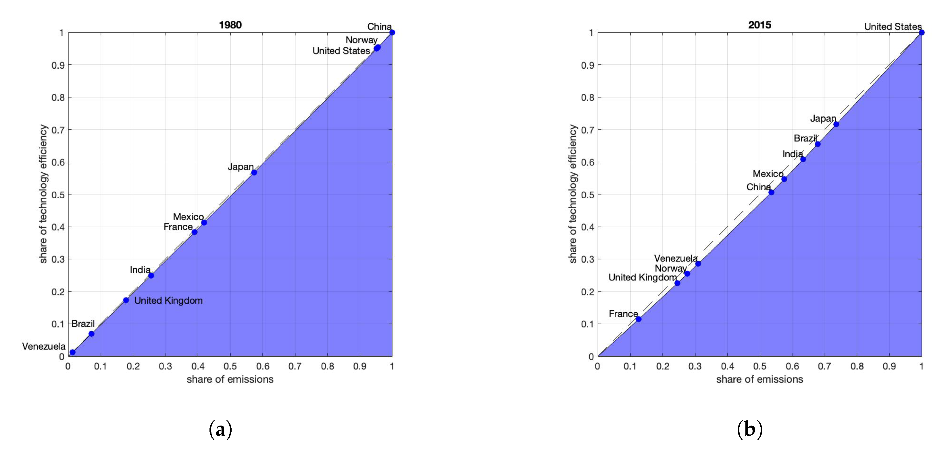
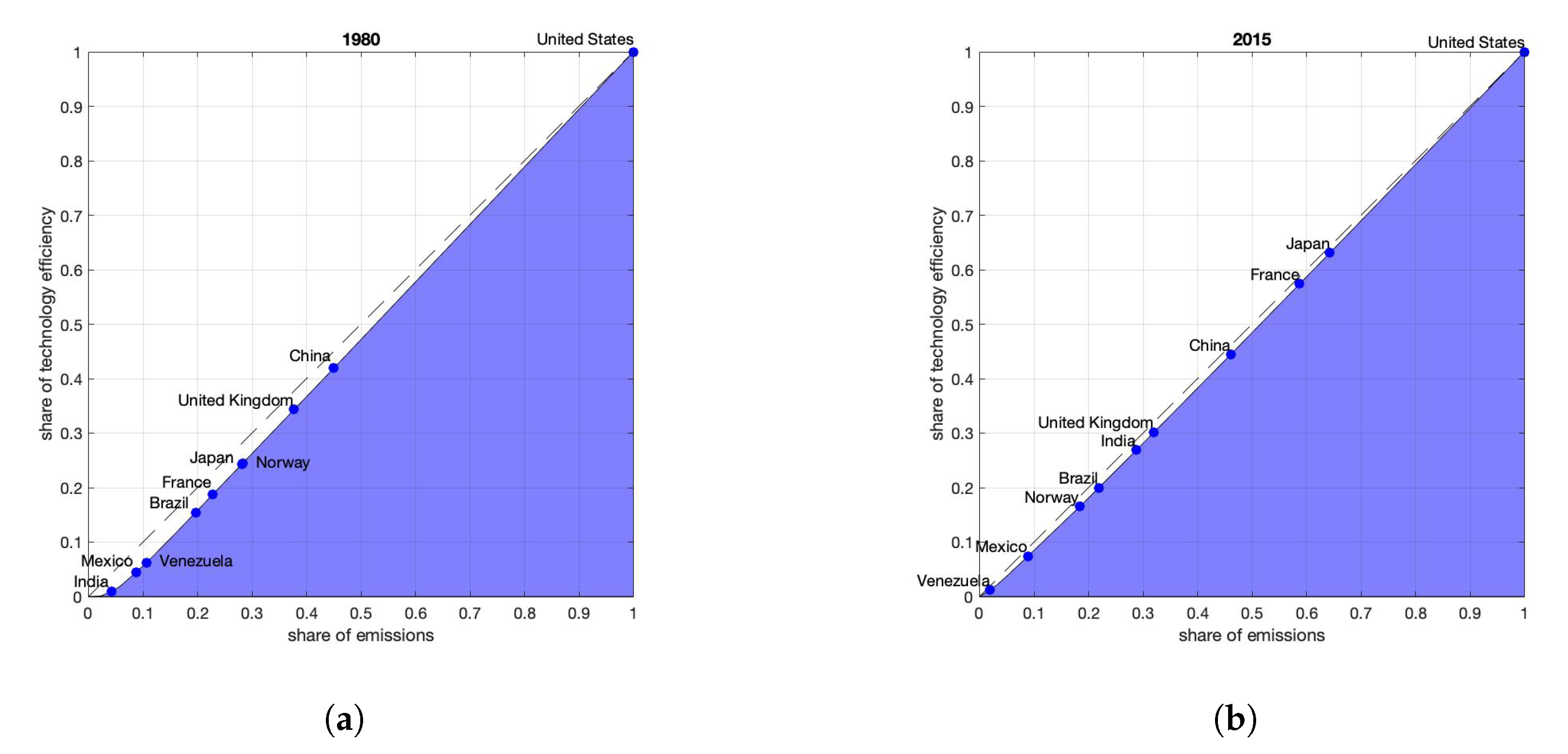
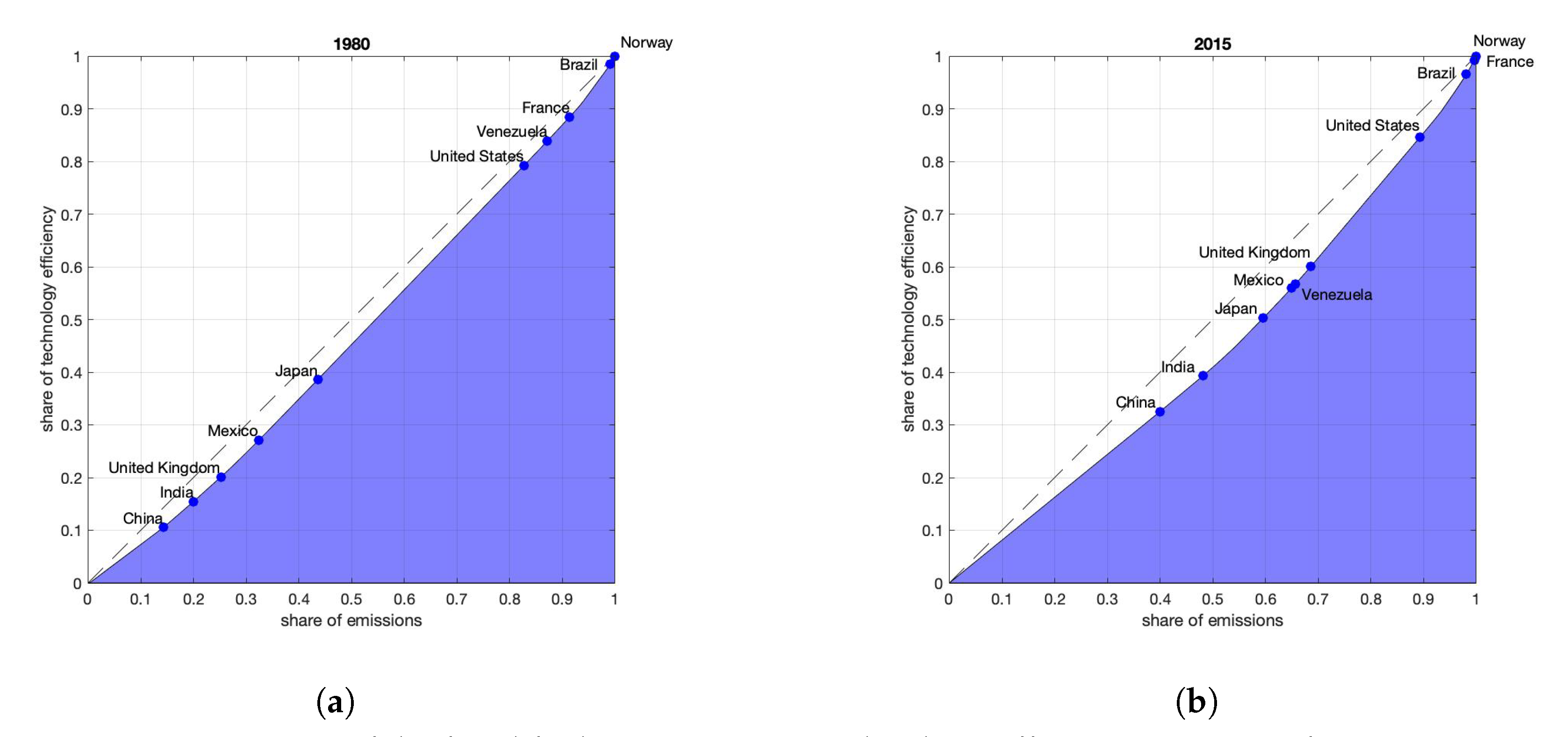
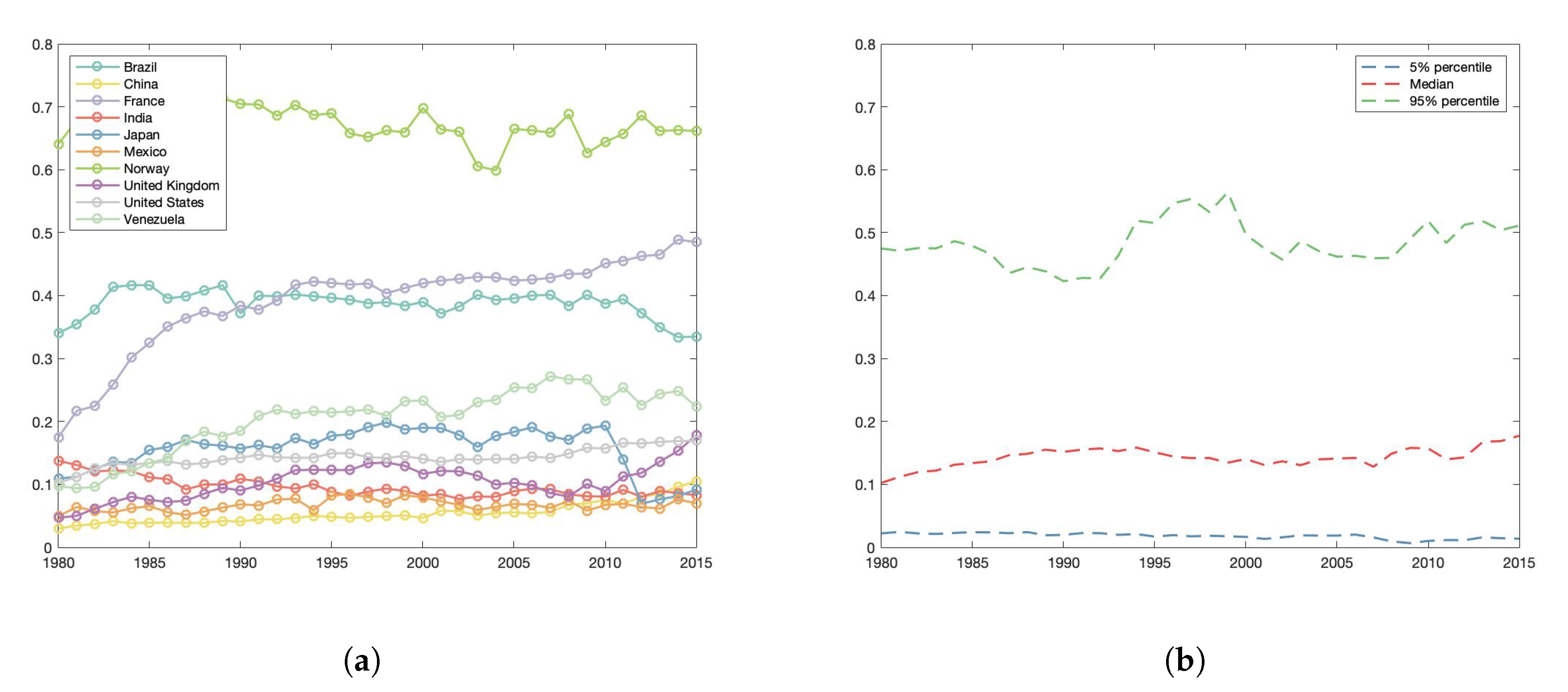
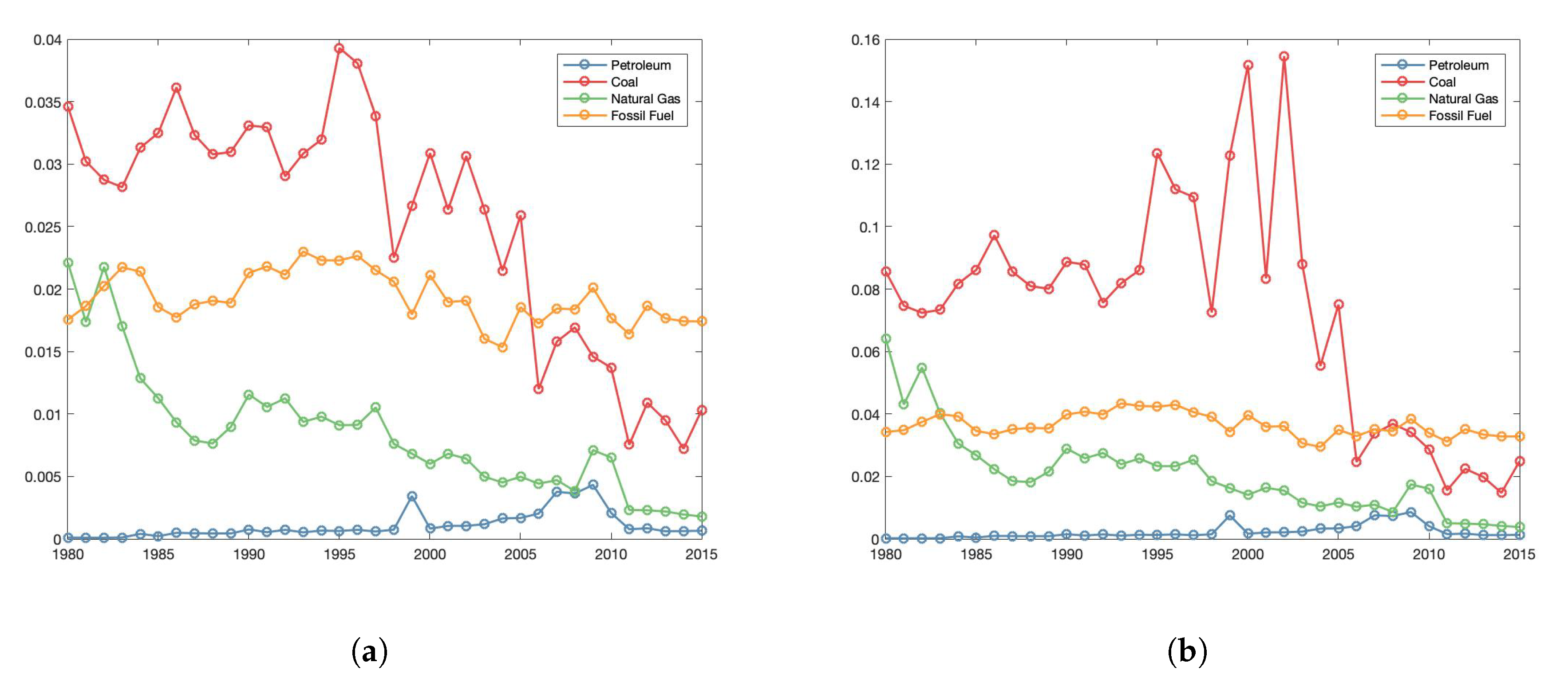
3.1. Consumption Technology Efficiency in Terms of CO₂ Emissions

Regarding fossil primary energy sources, we consider petroleum, coal, and natural gas. We present the consumption technology efficiency in terms of CO₂ emissions along time in Figure 1, Figure 2, Figure 3 and Figure 4 for petroleum, coal, natural gas, and fossil fuel, respectively. For each case, we present technology efficiencies for a selected group of countries, also including the median, $5\%$ percentile, and $95\%$ percentile of the entire set of considered countries. This group of countries was selected based on data availability and their importance for a comparative analysis aiming to overcome misconceptions and prejudices already alluded to in the introduction.

Notice that, while the technology efficiency medians are relatively stable along time, the percentiles have different behaviors. The distance between the percentiles and the medians gives an intuitive idea of the global spread of technology efficiency along time.

In order to measure the global spread of technology efficiency, we first use the technology efficiency Gini index, computed from the corresponding Lorenz curve, and these are present in Figure 5, Figure 6, Figure 7 and Figure 8 for petroleum, coal, natural gas, and fossil fuels. For each case, we present the Lorenz curve for two dates: 1980 and 2015. In addition, we also indicate some of the countries in the figures for illustration purposes. Since the obtained Lorenz curves are very close to the diagonal line, we conclude that technology efficiency is nearly equally distributed between countries.

Using technology efficiency Lorenz curves for each year, we obtain evolution along time of this index. In Figure 9, we present the technology efficiency Gini indexes for petroleum, coal, natural gas, and fossil fuels. The obtained Gini indexes are numerically close to zero along time, indicating technology efficiencies nearly equally distributed between the countries. Moreover, while the equality of the technology efficiency for coal and natural gas between 1980 and 2015 seems to be improving, the opposite seems to occur for petroleum and fossil fuels. Fossil fuels are composed of petroleum, coal, and natural gas. However, since the Gini index does not satisfy the additive decomposability, it is not easy to grasp the relation between these those indexes.

In Figure 10a, we present the evolution along time of empirical global technology efficiency for consumption of petroleum, coal, natural gas, and fossil fuels. It is possible to notice that the global technology efficiency for the consumption of coal is stable along time while the global technology efficiencies for the consumption of petroleum and natural gas seem to slightly increase along time. During the considered time period, the global technology efficiency is highest for natural gas, and lowest for coal. In Figure 10b, we present the mean value, among countries, for the technology efficiency for the consumption of petroleum, coal, natural gas, and fossil fuels. Notice that the relative positions of countries for technology efficiency in fossil fuels consumption is (almost) the same in several of these plots.

In Figure 11, we present the technology efficiency generalized entropy indexes for petroleum, coal, natural gas, and fossil fuels. As a particular cases, we present the mean log deviation ($\alpha =0$) and the Theil ($\alpha =1$) indexes. It is interesting to notice how different the behavior of the obtained generalized entropy indexes compared with the obtained Gini indices is. Gini indexes seem to be smoother, and they do not clearly reflect our intuition coming from the observed percentiles in Figure 1, Figure 2, Figure 3 and Figure 4. For instance, the percentile band for petroleum consumption technology efficiency increases between 2005 and 2010. The increase in the percetile band indicates an increase in the global inquality of the technology efficiency spread. In this case, it is possible to notice that the corresponding generalized entropy indexes clearly indicate an increase in inequality between 2005 and 2010. For coal, the lower percentile band shrinks between 1995 and 2000 while the upper percentile band starts to increase between 2000 and 2005. It is important to notice that the corresponding Gini index shows a relatively smooth behavior while the corresponding generalized entropy indices clearly indicates an asymmetry in change of the global technology efficiency distribution.

In Figure 12, we present the technology efficiency Atkinson indexes for petroleum, coal, natural gas, and fossil fuels. As particular cases, we present the Atkinson indices for $ϵ=0.5$ and $ϵ=1$. It is possible to notice a similarity between Atkinson indexes and generalized entropy indexes. Atkinson indexes for lower values of $ϵ$ are quite similar to generalized entropy indexes for higher values of $\alpha$ and vice-versa. Either generalized entropy or Atkinson indexes becomes more sensitive to changes at the lower end of the technology efficiency distribution as, respectively, $\alpha$ approaches 0 and $ϵ$ approaches 1. The same behavior is observed for the upper end of the technology efficiency distribution as, respectively, $\alpha$ approaches 1 and $ϵ$ approaches 0.

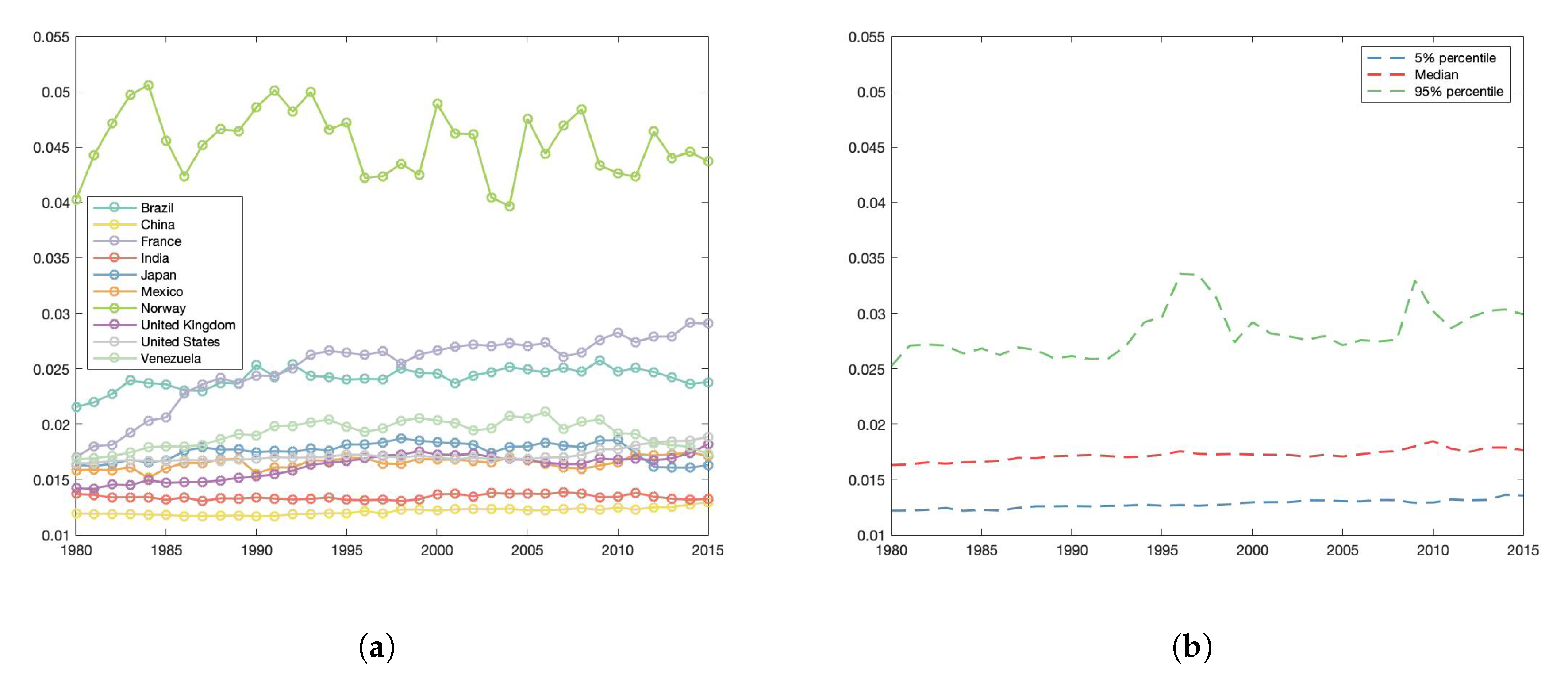
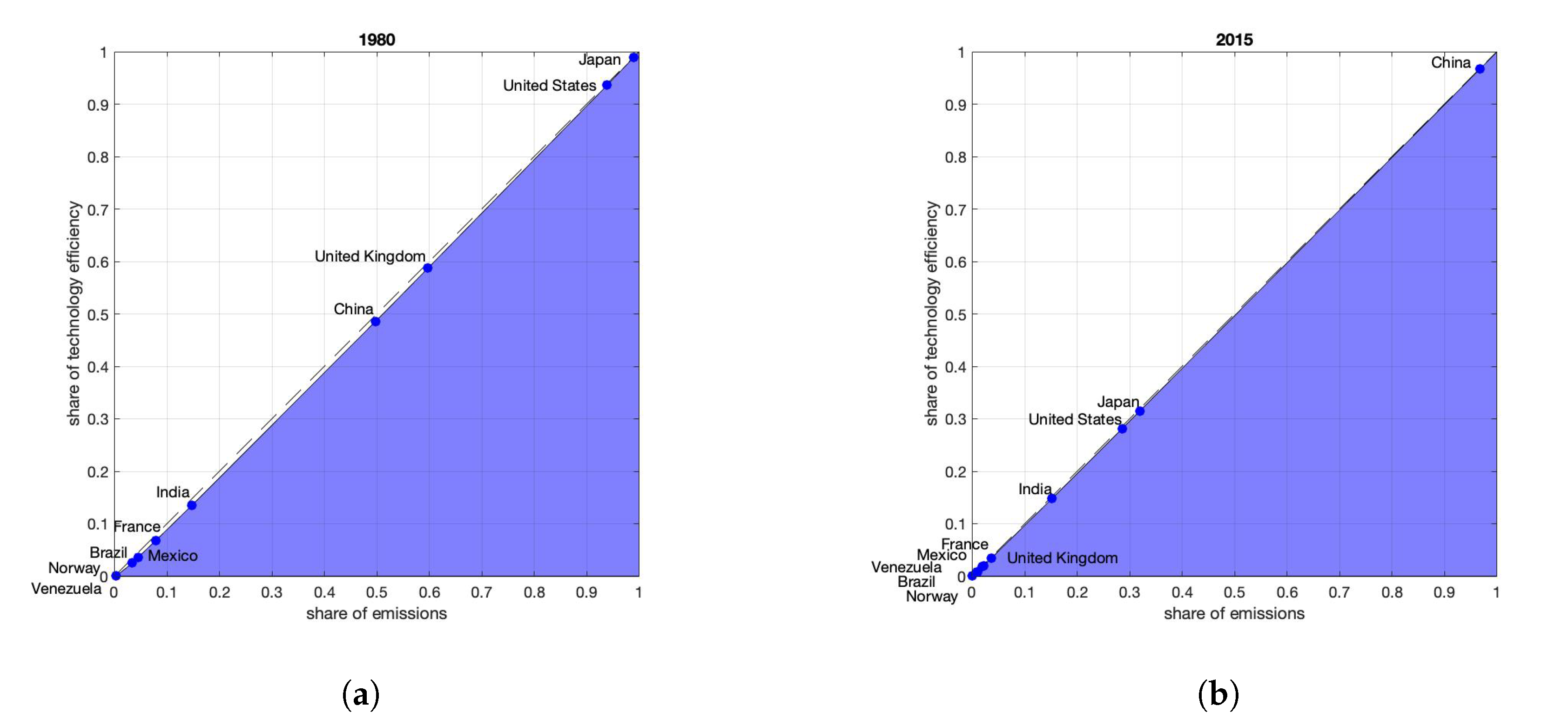
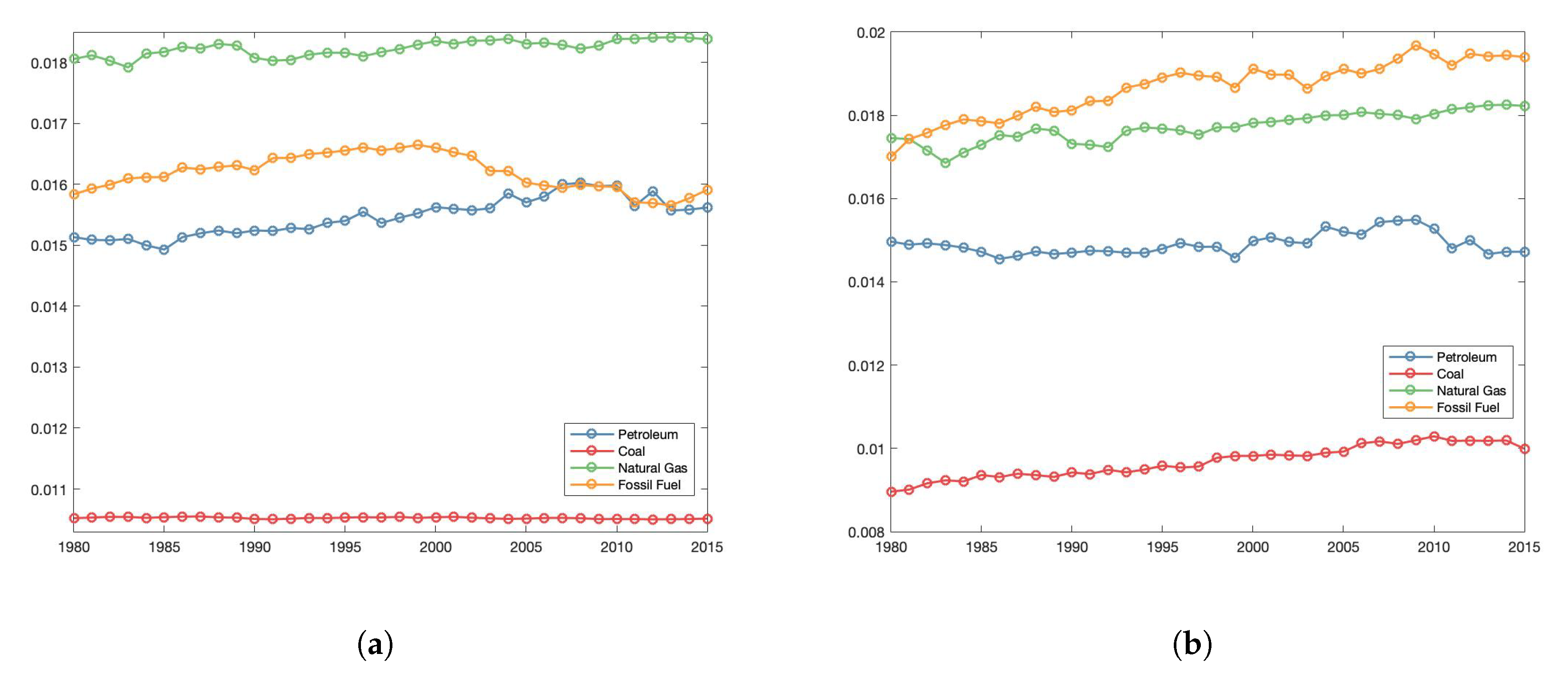
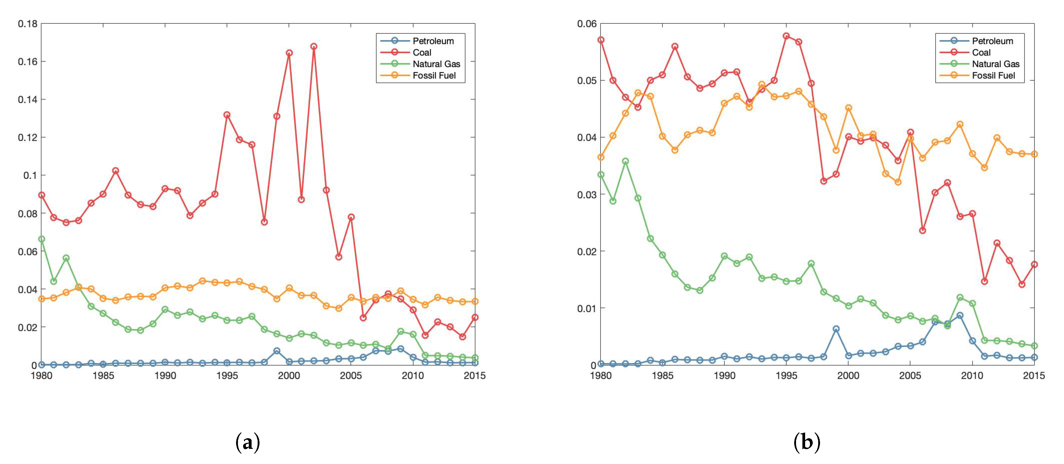
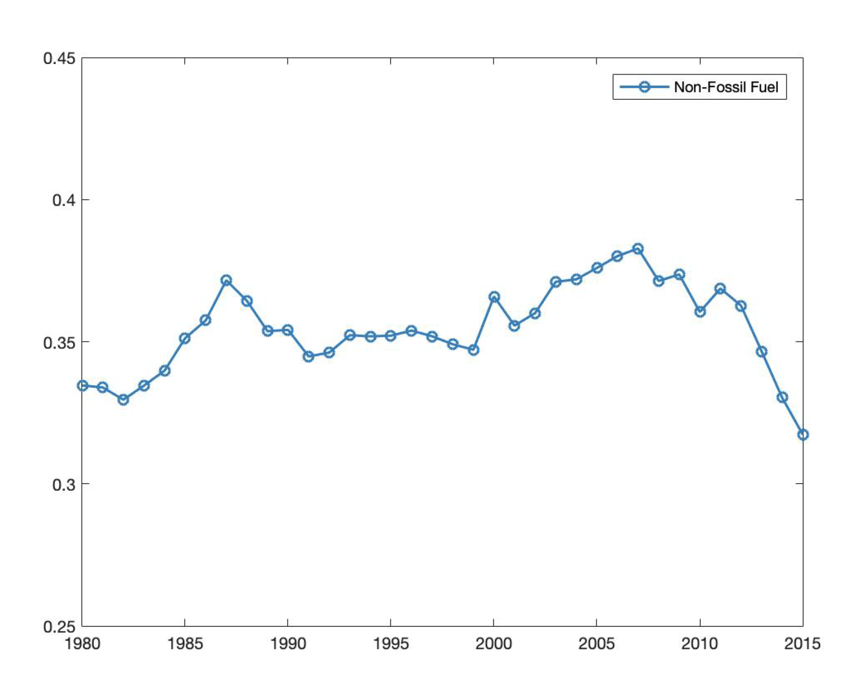
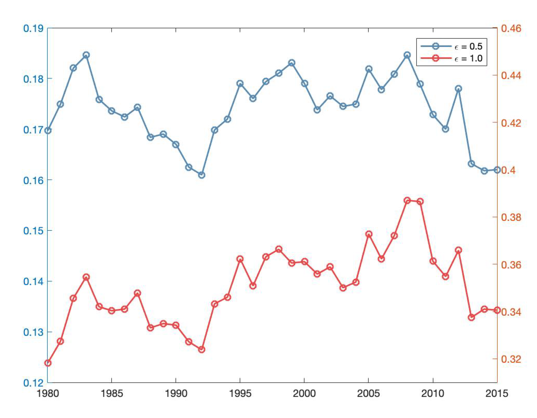
3.2. Non-Fossil Fuel Use Global Spread

This subsection focuses on global spreads in the use of non-fossil fuels. Figure 13 presents non-fossil fuel use for the same selected group of countries used in the last subsection and the median, $5\%$ percentile, and $95\%$ percentile for the entire set of considered countries. It is interesting to notice that the median value of use of non-fossil fuel increases comparing from 1980 to 2015. In addition, the lower percentile of these quantities seems to be more stable while the upper percentile presents a higher oscillation. The distance between the percentiles and the medians gives an intuitive idea of the global spread of use of non-fossil fuels along time. In the following paragraphs, we present our measures for global spread of use of non-fossils, based on Gini and generalized entropy indexes.

Non-fossil fuel Gini indexes are calculated from the corresponding Lorenz curves, as presented in Figure 14, for 1980 and 2015. The non-fossil fuels Gini index along time is presented in Figure 15. The technology efficiency Gini indexes for fossil fuels are close to zero, suggesting an almost homogeneous spread of technology efficiency among the different countries. In contrast, the non-fossil fuel Gini index is not close to zero, indicating a higher inequality of non-fossil fuel use between different countries.

In Figure 16, we present global non-fossil fuel use and its mean value among countries from 1980 to 2015. Notice that either global non-fossil fuel use or its mean value increases during the considered time interval. Moreover, the non-fossil fuel use mean value among countries is higher than global non-fossil fuel use during the considered time interval due to the existence of countries with lower non-fossil fuel use with higher energy consumption.

In Figure 17, we present the non-fossil fuel generalized entropy indexes for particular cases: the mean log deviation ($\alpha =0$) and the Theil index ($\alpha =1$). Notice the difference in behavior between generalized entropy indexes vs. Gini index. Intuitively, the generalized entropy indexes seem to better capture the percentiles behavior. For instance, in Figure 13b, between 1985 and 1995, there is a decrease in the $95\%$ percetile. By inspection, it is also possible to notice a decrease in the same time period of the generalized entropy indexes in Figure 17. However, in Figure 15, the Gini index seems to increase in the same time period. Finally, in Figure 17, it is possible to notice that the mean log deviation index increases between 1980 and 2015, while the Theil index decreases. Consequently, inequality increases during the considered time period at the lower end of the non-fossil fuel use distribution. In contrast, inequality decreases during the considered time period at the upper end of the non-fossil fuel use distribution.

In Figure 18, we present non-fossil fuel Atkinson indexes for $ϵ=0.5$ and $ϵ=1.0$. Notice the similarity between the Atkinson indexes and generalized entropy indexes from Figure 17. Atkinson indices for lower values of $ϵ$ are quite similar to the generalized entropy indexes for higher values of $\alpha$ and vice-versa. Either Atkinson or generalized entropy indexes for non-fossil fuels use confirms that, during 1980 and 2015, inequality increases at the lower end of the non-fossil fuel distribution and decreases at its upper end. In other words, the countries with higher non-fossil fuel use are getting more equally distributed in terms of non-fossil fuel participation in total energy consumption. In contrast, countries with lower non-fossil fuel use are getting more unequally distributed.

Either technology efficiency and non-fossil fuels use are related to CO₂ emissions, and they are influenced by government policies and other possible common factors. Consequently, we investigate the relationship between changes in the global spread of technology efficiency and changes in the global spread of non-fossil fuels use using the following linear regression models

$$G_{{\epsilon }_t^{\mathrm{fossil} \mathrm{fuel}}}-G_{{\epsilon }_{t-1}^{\mathrm{fossil} \mathrm{fuel}}}=a_G\left(G_{{\rho }_t}-G_{{\rho }_{t-1}}\right)+b_G,$$

(27)

$$E_{{\epsilon }_t^{\mathrm{fossil} \mathrm{fuel}}}^{\alpha }-E_{{\epsilon }_{t-1}^{\mathrm{fossil} \mathrm{fuel}}}^{\alpha }=a_E^{\alpha }\left(E_{{\rho }_t}^{\alpha }-E_{{\rho }_{t-1}}^{\alpha }\right)+b_E^{\alpha }$$

(28)

and

$$A_{{\epsilon }_t^{\mathrm{fossil} \mathrm{fuel}}}^{ϵ}-A_{{\epsilon }_{t-1}^{\mathrm{fossil} \mathrm{fuel}}}^{ϵ}=a_A^{ϵ}\left(A_{{\rho }_t}^{ϵ}-A_{{\rho }_{t-1}}^{ϵ}\right)+b_A^{ϵ},$$

(29)

where $a_G$, $b_G$, $a_E^{\alpha }$, $b_E^{\alpha }$, $a_A^{ϵ}$, and $b_A^{ϵ}$ are coefficients to be estimated. In

Table 1. Estimation of coefficients for the linear regression models (27)–(29).

Coefficient	Estimate	p-Value	Standard Error	t-Statistic
$a_G$	0.155	0.017	0.062	2.513
$b_G$	0.001	0.033	0.001	2.230
$a_E^{\alpha =0.0}$	0.084	0.002	0.025	3.408
$b_E^{\alpha =0.0}$	−0.000	0.782	0.000	−0.279
$a_E^{\alpha =1.0}$	0.077	0.207	0.059	1.288
$b_E^{\alpha =1.0}$	0.000	0.853	0.001	0.186
$a_A^{ϵ=0.5}$	0.118	0.027	0.051	2.316
$b_A^{ϵ=0.5}$	0.000	0.933	0.000	0.085
$a_A^{ϵ=1.0}$	0.126	0.002	0.037	3.400
$b_A^{ϵ=1.0}$	−0.000	0.777	0.000	−0.286

, we present the estimated coefficients using ordinary least squares with the corresponding p-values, standard errors and t-statistics. In

Table 2. Statistics for the linear regression models (27)–(29).

Equation	${\mathit{R}}^2$	Adjusted ${\mathit{R}}^2$	p-Value	F-Statistic	Root Mean Squared Error
(27)	0.161	0.135	0.017	6.320	0.003
(28) with $\alpha =0.0$	0.260	0.238	0.002	11.600	0.003
(28) with $\alpha =1.0$	0.048	0.019	0.207	1.660	0.004
(29) with $ϵ=0.5$	0.140	0.114	0.027	5.360	0.002
(29) with $ϵ=1.0$	0.259	0.237	0.002	11.600	0.003

, we present some statistics of the estimated linear regression models: $R^2$, adjusted $R^2$, p-value, F-statistic, and root mean squared error. Notice that the estimated values for $a_G$, $a_E^{\alpha }$, and $a_A^{ϵ}$ are all positive despite the fact that the significance of the results depends on each case. Consequently, we can attest to a positive relationship between changes in global spreads of the technology efficiency and changes in global spreads of non-fossil fuels use for the major part of the cases. In this respect, from Table 2, it is also possible to notice that model (28) with $\alpha =0.0$ indicates a stronger positive relation than model (28) with $\alpha =1.0$. In other words, the first model has a higher $R^2$, higher adjusted $R^2$, higher F-statistic, lower p-value, and lower root mean squared error. Analogously, model (29) with $ϵ=1.0$ indicates a stronger positive relation than model (29) with $ϵ=0.5$, because the first model has a higher $R^2$, higher adjusted $R^2$, higher F-statistic, and lower p-value. Since either generalized entropy or Atkinson indexes become more sensitive to changes at the lower end of technology efficiency and non-fossil fuels use distributions as $\alpha$ approaches 0 and $ϵ$ approaches 1, we conclude that an attested positive relation between changes in global spreads of technology efficiency and changes in global spreads of non-fossil fuels use is higher at the lower end of the distributions.

4. Conclusions

Our main contribution in this paper is the introduction of novel index measures for global spread in primary energy consumption technology efficiency and non-fossil fuel use; these index measures are based on the Gini index and on generalized entropy indexes. In the empirical studies conducted in this paper, our novel index measures were able to capture interesting correlations or associations between several quantities of interest and their global spreads. Careful analysis of these and similar relations should prove important for strategic planning and allocation of capital and other resources by state entities, investment and energy firms, and other interested parties. For instance, in a global carbon credit context, such measures could help to verify the effectiveness of the policies for the regions buying or selling carbon credits in terms of decreasing the global spread of technology efficiency and non-fossil fuel use over time.

The Lorenz curves and the Gini indices for the technology efficiency of petroleum, coal, natural gas, and fossil fuel show the relative equality in their global spread along time. Empirically, we observe that the Gini indices are smoother than the generalized entropy indices, and the generalized entropy indices seem to reflect better the intuition that comes from the observed percentiles of the data. Compared with the Gini indices, the generalized entropy indices satisfy the additive decomposability and they have a parameter to adjust the metric to be more sensitive to the lower or upper ends of the technology efficiency distribution. In particular, we also present the Atkinson indices for technology efficiency. The Atkinson indices are particular cases of the generalized entropy indices.

Compared with the technology efficiency case, the Lorentz curves and the Gini indices for non-fossil fuel use indicate higher inequality between the different countries along time. Empirically, we observe that generalized entropy indices capture better the percentiles behavior of the data compared with the Gini index. The generalized entropy indices indicate that the inequality increases during the considered time period at the lower end of non-fossil fuel use distribution while inequality decreases during the considered time period at the upper end of non-fossil fuel use distribution. In other words, countries with higher non-fossil fuel use are getting more equally distributed in terms of non-fossil fuel participation in the total energy consumption. On the other hand, countries with lower non-fossil fuel use are getting more unequally distributed.

Technology efficiency and non-fossil fuel use are related to CO₂ emissions, and they are influenced by government policies and other possible common factors. In this paper, we identify a positive relationship between the changes in the global spread of technology efficiency and the changes in the global spread of non-fossil fuel use. Actually, the positive relationship between changes in the global spread of technology efficiency and changes in the global spread of non-fossil fuel use is higher at the lower end of the distributions. In other words, the identified positive relationship is higher for countries with lower technology efficiency and lower non-fossil fuel use.

The empirical studies in this paper were conducted paying special attention to global spreads of technology efficiency and non-fossil fuels use. As application guidelines, the generalized entropy and Atkinson-based measures are better suited than Gini index-based measure when aiming for greater sensitivity at the lower or upper ends of the distributions of interest, like technology efficiency or non-fossil fuel use. Nevertheless, the methodology developed in this paper could also be applied to different studies, for example, comparing the development of different regions in a single country. Furthermore, studies of global spreads of fuel use could be extended to other primary energy sources and could be used in the context of non-primary energy consumption. In future works, we plan to pursue these lines of research, always aiming for a cleaner and more sustainable world.

References

1. BP. BP Statistical Review of World Energy; BP: London, UK, 2019. [Google Scholar]
2. United Nations. Emissions Gap Report; United Nations Environment Programme: Nairobi, Kenya, 2018.
3. International Energy Agency. World Energy Outlook 2018; International Energy Agency: Paris, France, 2018. [Google Scholar]
4. Awerbuch, S.; Berger, M. Applying Portfolio Theory to EU Electricity Planning and Policy-Making; International Energy Agency/Emerging Energy Technologies: Paris, France, 2003. [Google Scholar]
5. Awerbuch, S. Portfolio-based electricity generation planning: Policy implications for renewable and energy security. Mitig. Adapt. Strateg. Glob. Chang. 2006, 11, 693–710. [Google Scholar] [CrossRef]
6. Marrero, G.A.; Ramos-Real, F.J. Electricity generation cost in isolated system: The complementarities of natural gas and renewables in the canary islands. Renew. Sustain. Energy Rev. 2010, 14, 2808–2818. [Google Scholar] [CrossRef] [Green Version]
7. Losekann, L.; Marrero, G.A.; Ramos-Real, F.J.; Almeida, E.L.F. Efficient power generating portfolio in Brazil: Conciliating cost, emissions and risk. Energy Pol. 2013, 62, 301–314. [Google Scholar] [CrossRef]
8. Marrero, G.A.; Puch, L.A.; Ramos-Real, F.J. Mean-variance portfolio methods for energy policy risk management. Int. Rev. Econ. Financ. 2015, 40, 246–264. [Google Scholar] [CrossRef]
9. Costa, O.L.V.; Ribeiro, C.O.; Rego, E.E.; Stern, J.M.; Parente, V.; Kileber, S. Robust portfolio optimization for electricity planning: An application based on the Brazilian electricity mix. Energy Econ. 2017, 64, 158–169. [Google Scholar] [CrossRef]
10. Takada, H.H.; Stern, J.M.; Costa, O.L.V.; Ribeiro, C.O. Classical-equivalent Bayesian portfolio optimization for electricity generation planning. Entropy 2018, 20, 42. [Google Scholar] [CrossRef] [Green Version]
11. Gini, C. Variabilità e Mutabilità: Contributo allo Studio delle Distribuzioni e delle Relazioni Statistiche; Facoltá di Giurisprudenza della Regia Università di Cagliari, Tipografia di Paolo Cuppini: Bologna, Italy, 1912. [Google Scholar]
12. Heil, M.T.; Wodon, Q.T. Inequality in CO2 emissions between poor and rich countries. J. Environ. Dev. 1997, 6, 426–452. [Google Scholar] [CrossRef]
13. Heil, M.T.; Wodon, Q.T. Future inequality in CO2 emissions and the impact of abatement proposals. Environ. Resour. 2000, 17, 163–181. [Google Scholar] [CrossRef]
14. Groot, L. Carbon Lorenz curve. Resour. Energy Econ. 2010, 32, 45–64. [Google Scholar] [CrossRef]
15. Teng, F.; He, J.; Pan, X.; Zhang, C. Metric of carbon equity: Carbon Gini index based on historical cumulative emission per capita. Adv. Clim. Chang. Res. 2011, 2, 134–140. [Google Scholar] [CrossRef]
16. Lawrence, S.; Liu, Q.; Yakovenko, V.M. Global inequality in energy consumption from 1980 to 2010. Entropy 2013, 15, 5565–5579. [Google Scholar] [CrossRef] [Green Version]
17. Jacobson, A.; Milman, A.D.; Kammen, D.M. Letting the (energy) Gini out of the bottle: Lorenz curves of cumulative electricity consumption and Gini coefficients as metrics of energy distribution and equity. Energy Pol. 2005, 33, 1825–1832. [Google Scholar] [CrossRef]
18. Druckman, A.; Jackson, T. Measuring resource inequalities: The concepts and methodology for an area-based Gini coefficient. Ecol. Econ. 2008, 65, 242–252. [Google Scholar] [CrossRef] [Green Version]
19. Soares, T.C.; Fernandes, E.A.; Toyoshima, S.H. The CO2 emission Gini index and the environmental efficiency: An analysis for 60 leading world economies. EconomiA 2018, 19, 266–277. [Google Scholar] [CrossRef]
20. Shorrocks, A.F. The class of additively decomposable inequality measures. Econometrica 1980, 48, 613–625. [Google Scholar] [CrossRef] [Green Version]
21. Bourguignon, F. Decomposable income inequality measures. Econometrica 1979, 47, 901–920. [Google Scholar] [CrossRef] [Green Version]
22. Sauerbrei, S. Lorenz curves, size classification, and dimensions of bubble size distributions. Entropy 2010, 12, 1–13. [Google Scholar] [CrossRef] [Green Version]
23. Atkinson, A.B. On the measurement of inequality. J. Econ. Theory 1970, 2, 244–263. [Google Scholar] [CrossRef]
24. Milanović, B. Worlds Apart: Measuring International and Global Inequality; Princeton University Press: Princeton, NJ, USA, 2007. [Google Scholar]
25. US Energy Information Administration (EIA): International Energy Statistics. Available online: http://www.eia.gov (accessed on 15 November 2019).
Figure 1. Petroleum consumption technology efficiency in terms of CO2 emissions for (a) a sample of countries and (b) the set’s median, 5% percentile, and 95% percentiles.
Energies 13 04938 g001
Figure 2. Coal consumption technology efficiency in terms of CO2 emissions for (a) a sample of countries and (b) the set’s median, 5% percentile, and 95% percentile.
Energies 13 04938 g002
Figure 3. Natural gas consumption technology efficiency in terms of CO2 emissions for (a) a sample of countries and (b) the set’s median, 5% percentile, and the 95% percentile.
Energies 13 04938 g003
Figure 4. Fossil fuels consumption technology efficiency in terms of CO2 emissions for (a) a sample of countries and (b) the set’s median, 5% percentile, and 95% percentile.
Energies 13 04938 g004
Figure 5. Lorenz curve of the petroleum consumption technology efficiency in terms of CO2 emissions in (a) 1980 and (b) 2015.
Energies 13 04938 g005
Figure 6. Lorenz curve of the coal consumption technology efficiency in terms of CO2 emissions in (a) 1980 and (b) 2015.
Energies 13 04938 g006
Figure 7. Lorenz curve of the natural gas consumption technology efficiency in terms of CO2 emissions in (a) 1980 and (b) 2015.
Energies 13 04938 g007
Figure 8. Lorenz curve of the fossil fuels consumption technology efficiency in terms of CO2 emissions in (a) 1980 and (b) 2015.
Energies 13 04938 g008
Figure 9. Technology efficiency Gini indexes for petroleum, coal, natural gas, and fossil fuels.
Energies 13 04938 g009
Figure 10. (a) The empirical global technology efficiency for the consumption of petroleum, coal, natural gas, and fossil fuel along time, ε ^ t m and (b) the mean between the countries of the technology efficiency for the consumption of petroleum, coal, natural gas, and fossil fuel along time, ε ¯ t m .
Energies 13 04938 g010
Figure 11. Technology efficiency generalized entropy indices for petroleum, coal, natural gas, and fossil fuel using (a) α = 0 (mean log deviation index) and (b) α = 1 (Theil index).
Energies 13 04938 g011
Figure 12. Technology efficiency Atkinson indexes for petroleum, coal, natural gas, and fossil fuels using (a) ϵ = 0.5 and (b) ϵ = 1.
Energies 13 04938 g012
Figure 13. Non-fossil fuel use for (a) a sample of countries and (b) the median, 5% percentile, and 95% percentile.
Energies 13 04938 g013
Figure 14. Lorenz curve of non-fossil fuels use in (a) 1980 and (b) 2015.
Energies 13 04938 g014
Figure 15. Non-fossil fuels Gini index.
Energies 13 04938 g015
Figure 16. Global non-fossil fuel use and mean value among countries.
Energies 13 04938 g016
Figure 17. Non-fossil fuel use generalized entropy indices: mean log deviation index (α = 0) and Theil index (α = 1).
Energies 13 04938 g017
Figure 18. Non-fossil fuels use Atkinson indexes for ϵ = 0.5 (right axis) and ϵ = 1.0 (left axis).
Energies 13 04938 g018